Abstract
Accurate power curve modeling is essential to continuously evaluate the performance of a wind turbine (WT). In this work, we characterize the wind power curves using SCADA data acquired at a frequency of 5 min in a wind farm (WF) consisting of five WTs. Regarding the non-parametric methods, we select artificial neural networks (ANNs) to make curve estimations. Given that, we have the curves provided by the manufacturer of the WTs given by some very precisely measured pair of wind speed and power points. We can evaluate the difference between the manufacturer characterization and the ones estimated with the data provided by the SCADA system. Before the estimation, we propose a method of filtering the anomalies based on the characteristics provided by the manufacturer. We use three-quarters of the available data for curve estimation and one-quarter for the test. One WT suffered a break in the test part, so we can check how the test estimates reflect this problem in its wind-power curve compared to the estimations obtained in the WTs that worked adequately.
1. Introduction
The world’s needs for cleaner and renewable energy show no signs of slowing down, leaving markets seeking immediate solutions. Researchers face a daunting task: discovering ways to meet this ever-growing demand. Wind energy offers a promising possibility, particularly with the proliferation of wind farms.
While advances in wind technology are encouraging, many existing farms were built hastily, neglecting crucial long-term maintenance considerations.
Given that an essential part of the costs of generating wind energy originates in wind farms’ operation and maintenance stage, the most relevant line of action is making wind energy more competitive by reducing these costs. Once the WFs are built, O&M costs are the few parts of the process involved in generating wind power that can be addressed. To do so, condition-based maintenance (CBM) is considered one of the best solutions [1]. Supervisory control and data acquisition (SCADA) systems are used for data collection in wind farms, providing operational and condition information about wind turbines. These systems collect information from sensors distributed over different parts of the WT and provide the recorded captures’ maximum, minimum, average, and standard deviation values every 5/10 min. Although the SCADA systems were not originally designed to perform WTs prognosis, due to their wide availability and low cost (since we found them installed), much research has been generated to take advantage of their data.
As is well known, WTs are highly non-linear systems. One of the simplest and most efficient ways used by the manufacturers of WTs to characterize their performance is through the curve that relates the power generated as a function of the wind speed. These curves have four zones. The wind turbines do not generate power in zone 1, corresponding to low speeds. In zone 2, above a wind speed value, the generated power increases as the wind increases. In zone 3, the wind turbine generates its nominal power, and even if the wind speed continues to increase, the generated power remains constant. In zone 4, from a critical wind speed, the wind turbine stops for safety.
Given a wind speed profile, the power curve is used for the planning and development of wind farms and, as it is known that the malfunction of a wind turbine can drastically reduce its power generation capacity, and that the fact is reflected in this curve, it is also used to diagnose its health [2,3]. WT manufacturers certify these curves for specific wind conditions and turbine types, including air density and temperature at tower height. The International Electrotechnical Commission (IEC) standard 61400-12-1 [4] describes the certification process for measuring and recording a single turbine’s power performance characteristics. In practice, the power curve is constructed using historical data from the supervisory control and data acquisition (SCADA) system, with several SCADA-based models proposed for this purpose [5,6,7]. It is not surprising, therefore, that among the various magnitudes captured by SCADA, wind speed and active power output have attracted the attention of researchers [7]. When the pair of wind speed and power points are plotted directly from the SCADA data, the points are distributed around the theoretical curve, exhibiting some dispersion due to measurement errors and showing variations from the curve of the manufacturer, among other causes, in the 5 min averages made by the SCADA system. In addition, from the representation of the power curves from the raw data, a set of points appears outside the expected area, far from the manufacturer-given points. In this context, we call such points anomalies. To correctly estimate the power curves, it is necessary to clean the data anomalies [8,9,10]. These anomalies remain after typical outlier detection based primarily on statistical techniques. Most of the applied filtering and anomaly detection techniques are still based on statistical criteria and apply rules based on interquartile ranges (IQRs), or other statistical measures such as skewness or kurtosis, or more sophistical methods based on ML techniques such as self-organized maps (SOMs) and linear mixtures (LSOMs), which are unsupervised methods.
According to the literature [2], power curve modeling methods can be classified into discrete, deterministic/probabilistic, parametric/non-parametric, and based on the data used for modeling methods [2,3,11]. This work has focused on modeling power curves with non-parametric methods, as they are suitable for extracting models from large amounts of data. So, concerning modeling wind turbines’ power curves, the main non-parametric methods used explore artificial neural networks (ANN) [12], adaptive neuro-fuzzy inference system (ANFIS) [13,14], clustering [15], regression models, as well as different Machine Learning (ML) methods, such as support vector machine (SVM) and Gaussian Process (GP), due to their capabilities to modeling nonlinearities [16]. In addition, and in a very particular way to the estimation of power curves, copula models focus on learning the joint probability of wind speed and wind power [17].
As the estimation of power curves in wind turbines using SCADA data remains an active field, contributions are constantly made. Recently, improved estimations have been achieved mainly by the incremental sophistication of ML techniques. For example, in [18], super vector regressors are developed using a set of multivariate input features in which, in addition to mean variables, maximums, minimums and standard deviations provided by the SCADA are also considered. SVMs continue to be applied for a long time, as recently as in [19]. In [20], a deep learning technique based on convolutional neural networks (CNN) is introduced. To be able to train big networks, in this case, the authors first combine the action of multiple extreme learning machines (ELM) to increase the data dimensionality, followed by techniques to reduce redundant mapping before the application of CNNs. In general, data-driven ML-based methods exhibit a superior performance; however, they lack explainability, so a relevant line of research seeks to interpret the results in explainability, as in [21], or physical uncertainty quantification, as in [22]. Although most of the proposed estimators are data-driven, there are also contributions concerning parametric estimators, as in [23]. Due to the multiple contributions addressing the problem from different angles, it is always interesting to be aware of the latest state-of-the-art compilations, e.g., [24].
This work characterizes wind power curves using SCADA data, and is based on a new anomalies filtering technique approach and small artificial neural networks (ANNs) to estimate the curves. The filtering method introduced directly applies graphical information expressed as a condition to each pair of wind speed and power points. Removing such points using this method is fast. So, before making the estimation, a continuous power curve is obtained from the information provided by the WT manufacturer. The method we present is simple but effective, and especially practical compared to proposals appearing in the recent state of the art, where the dominant trend seems to add complexity to the methods. Although more complex methods can perform optimally in optimum conditions, they can face problems in real wind farm (WF) applications. Our method directly relates the two variables involved, the power and the wind speed, in the form of SCADA averages. A small-sized ANN performs well in the test without overfitting and requires only a few parameters to be tuned. That also requires less data to obtain a power curve estimation from new data, which helps to visualize possible changes faster. So, from our point of view, that is a valuable fact.
As for this work, we also have the curves of the particular WT model used in the experiments provided directly by the manufacturer; we can compare the characterization of the manufacturer concerning the estimated curves obtained from their estimation using the SCADA.
This work will be organized into Materials and Methods (Section 2), where we provide detailed descriptions of the following components: data used, Fuhrländer FL 2500/100 power curve provided by the manufacturer, anomaly filtering, and Wind Power curves estimation. The results are presented in Section 3, where we provide detailed descriptions of the following components: filtering and isolation of anomalies, using the filtered SCADA signals to estimate power curves, the training data, using the filtered SCADA signals to estimate power curves, and the test. Section 4 has a Discussion, and the main Conclusions are summarized in Section 5.
2. Materials and Methods
2.1. Data Used
This study utilizes a comprehensive three-year SCADA log from five 2.5 MW Fuhrläender FL2500 wind turbines. The SCADA system employs the IEC 61400-25 standard [25] communication protocol for transferring the wind turbine’s data and storing it in a MySQL database (DB). The database encompasses 312 analogue variables sourced from 78 different sensors. The initial DB entry commences on 1 January 2012 at 01:00, and concludes on 8 December 2014 at 06:00. The Fuhrläender FL2500 comprises various components, including the grid, transmission, generator, converter, nacelle, hydraulic system, rotor, meteorological unit, turbine, and tower. Signal categorization is organized into nine groups based on the specific system to which the signal pertains. Additionally, events and statistical parameters such as mean, standard deviation, maximum, and minimum values are documented at five-minute intervals. The used data are extracted from the database freely available at https://github.com/alecuba16/fuhrlander (accessed on 15 February 2024).
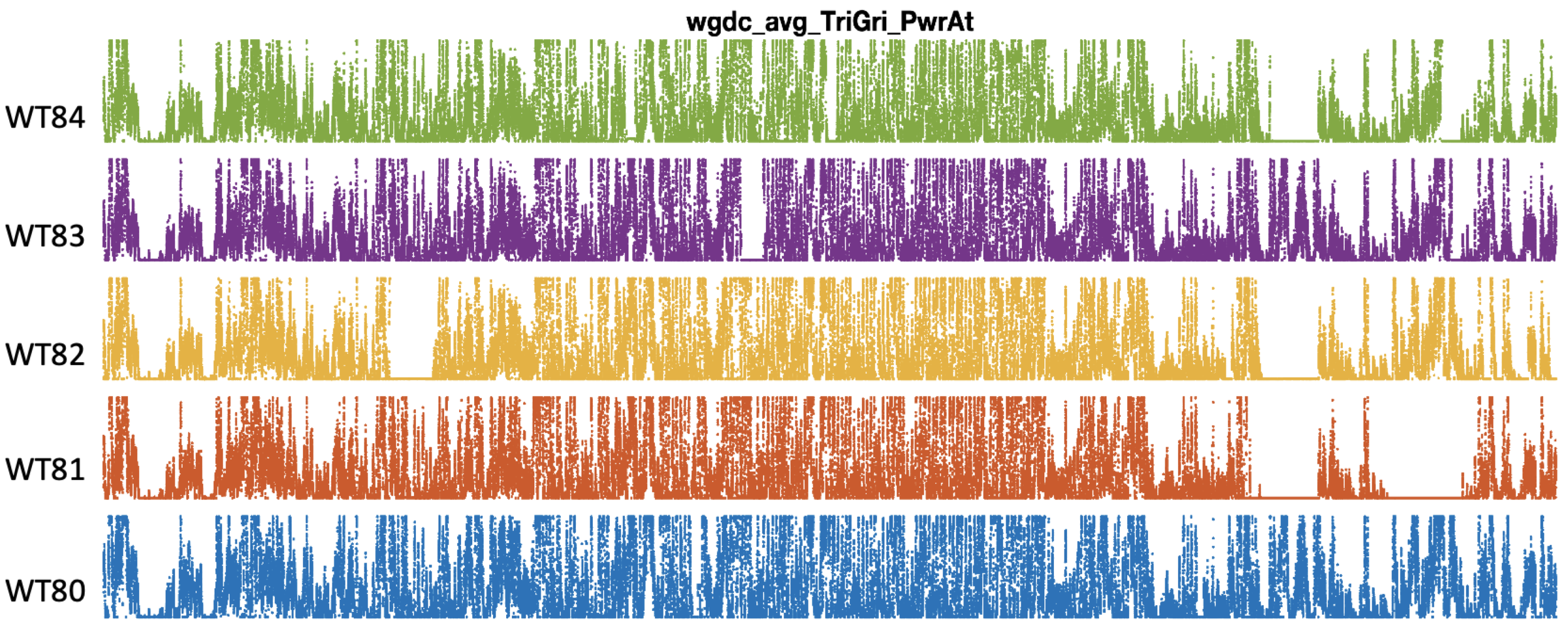
Of all the measurements provided by the SCADA system, we mainly use two signals that collect the wind and the power measured for each WT, with an additional signal to confirm whether the WT is active or not. We use the wgdc_avg_TriGri_PwrAt signal provided by the generator subsystem (wgdc) of each WT for active power measurements. For the wind speed, the signals wnac_avg_WSpd1 are obtained from each WT’s sensor in their Nacele system (wnac). Additionally, we use the rotation speed of the central axis of the turbine wgen_avg_RtrSpd_IGR in those cases where we need to verify that a WT is stopped despite high wind registers being measured. In all three signals, we use 5 min average (avg) values. We identify the five WTs with the following names: WT80, WT81, WT82, WT83 and WT84. Figure 1 shows the training portion of the wgdc_avg_TriGri_PwrAt signals, corresponding to the active power of each WT in the same temporal reference. The representation collects two-thirds of the total available signals. The third part is reserved for the test. Notice the strong similarity between signals, although it is occasionally observed that some WTs are not producing while the rest are.
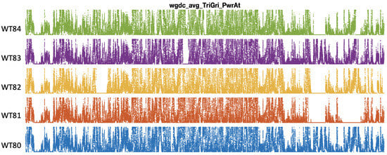
Figure 1.
Active power of each WT measured from the SCADA wgdc_avg_TriGri_PwrAt variable under the same temporal reference.
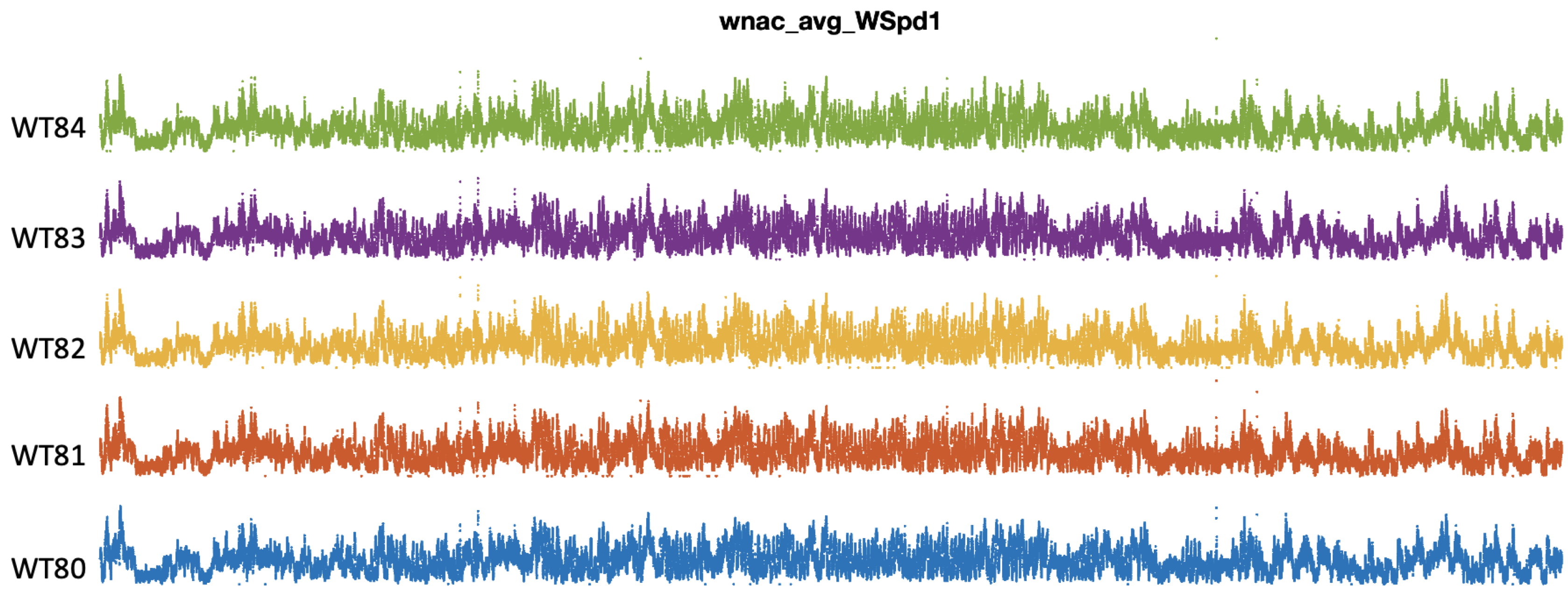
Figure 2 shows the training portion of the wnac_avg_WSpd1 signals, corresponding to the wind speed measured in the nacelle of each WT in the same temporal reference. As in Figure 1, the representation collects two-thirds of the available signals. We note the close similarities of the envelopes of the wind signals, much greater than the powers generated for each WT.
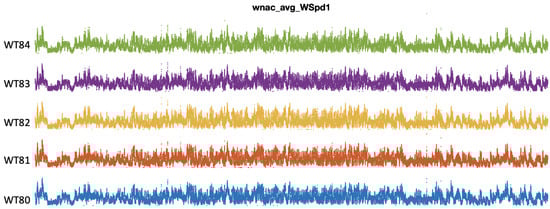
Figure 2.
Wind speed measured in the nacelle of each WT provided by the SCADA signals wnac_avg_WSpd1.
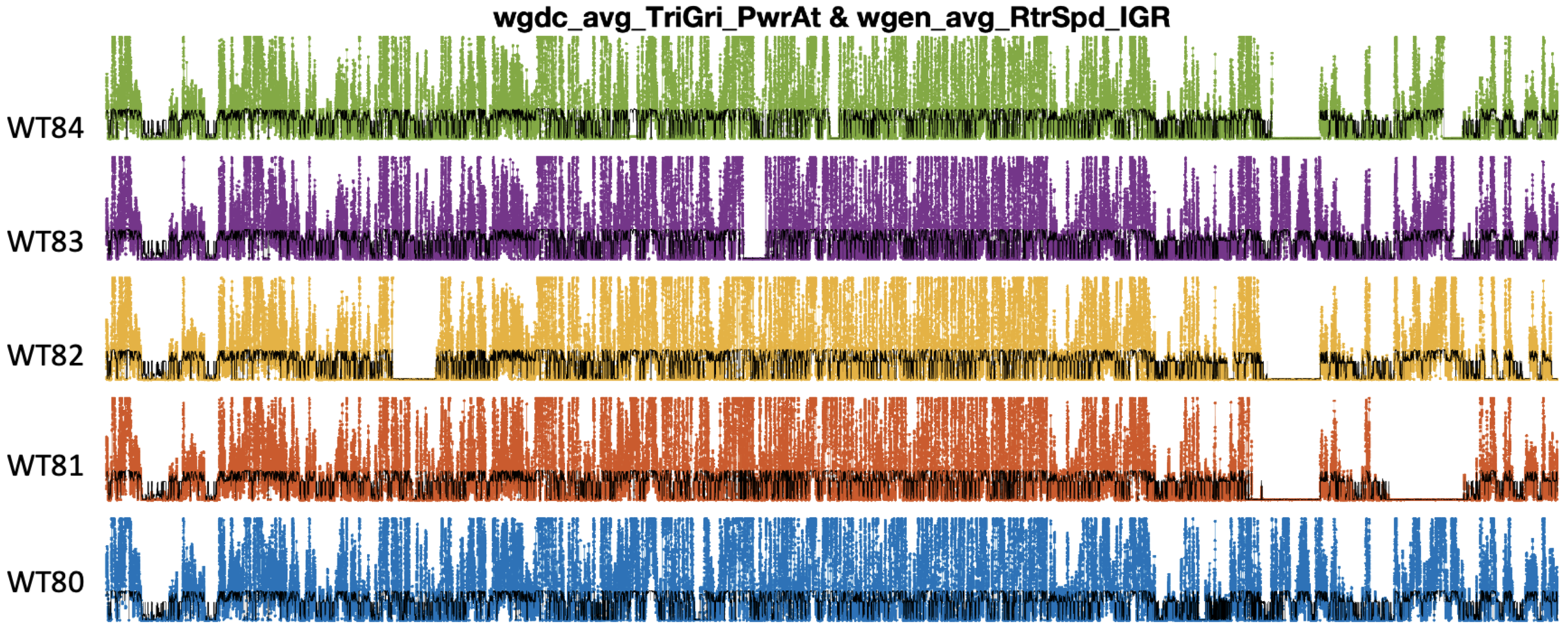
In Figure 3, for each WT, we superimpose over the signals wgdc_avg_TriGri_PwrAt the rotation speed of the rotors provided by wgen_avg_RtrSpd_IGR, which are represented scaled and in black color, to confirm that in the intervals where power is not produced, the WT is indeed also stopped. So, the data are consistent and reliable.

Figure 3.
Active power of each WT (wgdc_avg_TriGri_PwrAt) in different colors and a scaled version of their main axes rotation speed (wgen_avg_RtrSpd_IGR) in black, to verify the consistency o the SCADA data.
2.2. Fuhrländer FL 2500/100 Power Curve Provided by the Manufacturer
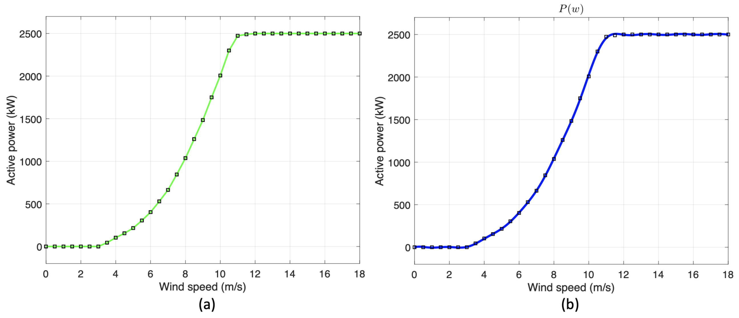
The Fuhrländer FL 2500/100 manufacturer characterizes the power generated with the wind speed of its WT model at increments of 0.5 m/s. One can find such data at https://www.thewindpower.net/turbine_en_154_fuhrlander_fl-2500-100.php (accessed on 15 February 2024). Notice that the manufacturer provides a set of 50 pairs of wind-power points measured precisely following the recommendations of the measurement protocol, but does not provide the intermediate values. Indeed, carrying out these measurements is expensive. In the left graph of Figure 4, one can see those points represented by small black squares. So, the function on the left of Figure 4, shown in green, is made by connecting the points provided by the manufacturer with straight lines. The green function is, therefore, a function defined by parts. To carry out the filtering we propose, we need a continuous function defined for any wind value, not only for the values provided by the manufacturer. If the interest was a continuous function defined by parts, a better alternative solution could be to use the third-order splines which, in addition to providing continuity at the points, would give continuity for the derivatives in such points. In this case, to manipulate functions defined by such a large number of parts makes them few operational. In the representation on the right of Figure 4, in blue, we show the continuous function used to have a power value for the wind speeds between the points provided by the manufacturer from the sum of only seven sinusoidal functions, so it is very compact. Previously, to decide the used curve, we compared techniques such as polynomial approximations of different orders, developments in the Fourier series, and even third-order splines to make this approximation. We discarded the third-order splines because we did not want to handle a piecewise function with such many parts. Of the contrasted approximations, the decomposition into sinusoidal functions is the one that provides better results in terms of RMSE, better even than the Fourier series for the same number of terms. Using sinusoidal functions, we have verified that seven sinusoidal terms obtain a better approximation than nine. For the approximation of the curve, we use the following expression:
where provides the power at the wind speed w. So, we particularize for . We represent the values of amplitudes , frequencies , and phases in Table 1.
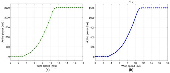
Figure 4.
(a) Points in (black squares) of the power curve provided by the manufacturer. (b) Continuous function in blue with the square points given by the manufacturer.

Table 1.
Coefficients of .
2.3. Anomaly Filtering
According to the distribution presented by these points (the anomalies), there are authors such as those of [9] who classify them according to three typologies: (1) power sensor failures, (2) wind speed sensors failure, or (3) due to the starting and stopping effect of the WT.
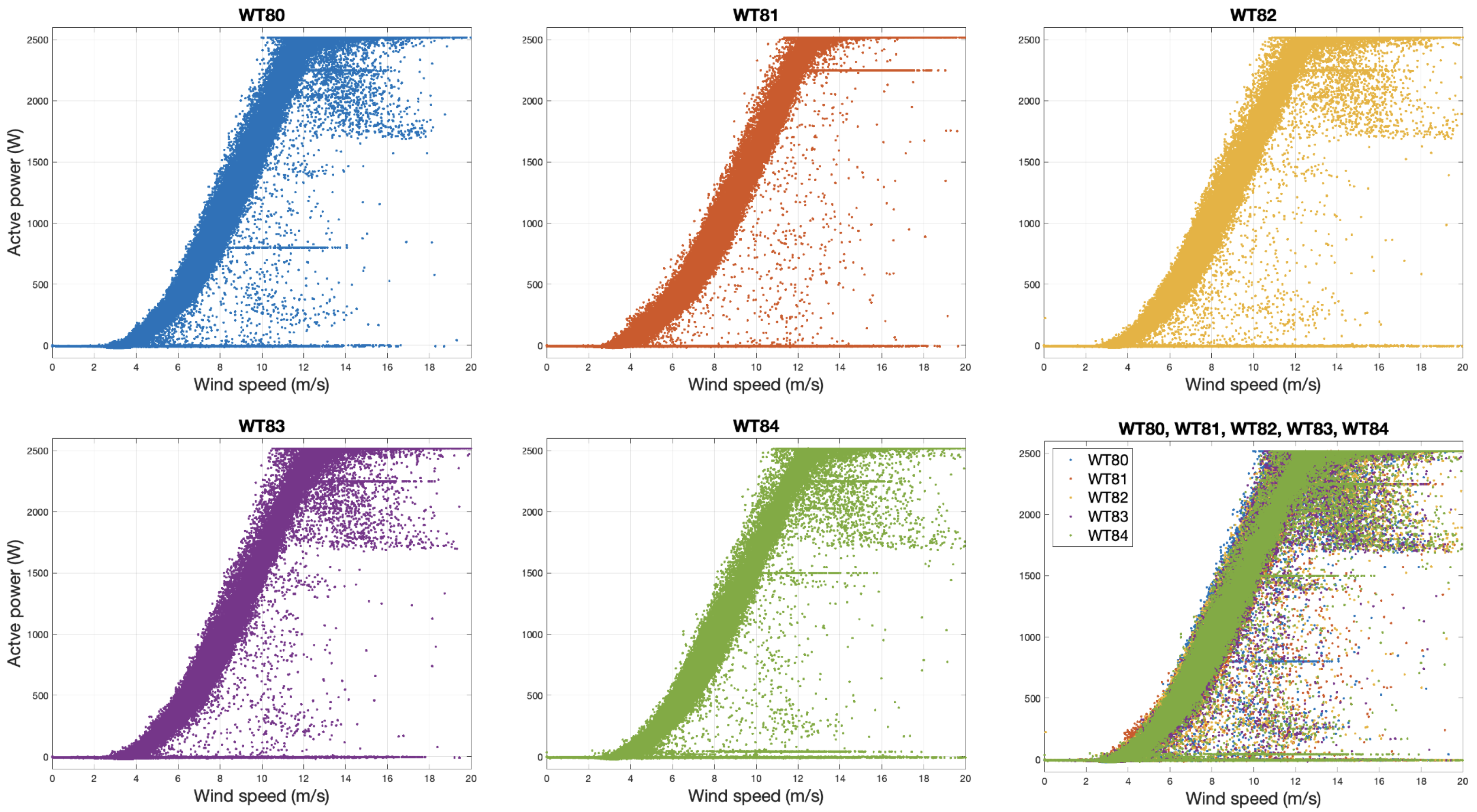
In Figure 5, we see represented the power curves of each WT resulting from directly crossing the wnac_avg_WSpd1 and wgdc_avg_TriGri_PwrAt signals provided by the SCADA. A total of 3/4 of the available signals are used. In some of these curves, anomalies appear, forming horizontal lines, which are attributed to failures of type (1), which are related to the power sensors. The anomalies distributed randomly inside the curves are of type (3), mainly attributed to the phenomenon of starting and stopping the WTs.
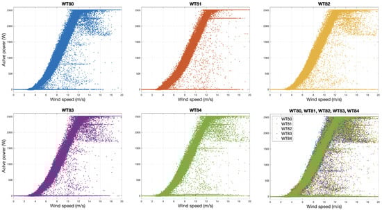
Figure 5.
Power curves of each WT resulting from directly crossing the wnac_avg_WSpd1 and wgdc_avg_TriGri_PwrAt signals. The last subplot is the superimposition of all the data of the 5 WTs.
In any case, the anomalies introduce errors in estimating the wind power curves. Before the estimation of the power curves of each WT, it is necessary to filter them.
When estimating the power curve from the data, what is evident from the related literature is the need to filter out anomalies to obtain decent estimates. This filtering determines the rest of the processing chain. The work in [24], which compiles recent state-of-the-art literature on estimating wind-power curves, devotes a section to anomaly classification and determines up to seven different types of anomalies, five of which are systematically treated in the texts. The other two appear less referenced. When discussing anomalies in the context of power curves, the texts systematically explain them graphically, and do so based on the graphical representation of the curve. However, the filtering process is usually based on more or less complicated statistical criteria although, we repeat, they are visually identified clearly in a graph.
Our approach may be surprisingly simple, but is very effective. It uses such graphical information. Since we only have the manufacturer’s information, we have an idea of the region of the graph where the points must appear. For the first filtering, we use such information. Since we know that the noise in the sensors, the different environmental conditions around the turbine (temperature, turbulence, humidity, etc.) and the averaging performed by the SCADA system generate some dispersion in the points around the curve, we select the candidate points in a margin around the nominal curve provided by the manufacturer. Since, as far as we know, the power performances, in practice, are usually slightly lower than those provided by the curve, we establish the criterion of selecting all the points that enter the region in the upper part represented in red in Figure 6. This red curve is made from the points provided by the manufacturer by shifting to the right and down a given distance.
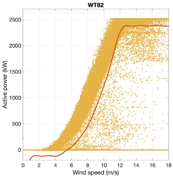
Figure 6.
Graphical interpretation of the anomaly filtering rule. The wind speed-active power pairs measured by the SCADA system are represented in yellow dots, and the line marking the filtering decision is in red.
So, to filter the data of each WT, we use the continuous manufacturer’s curve approximated by given in (1) that we move horizontally to the right and vertically down a distance . Considering the signals wnac_avg_WSpd1 and wgdc_avg_TriGri_PwrAt at the point k to be , , respectively, then if the following inequality is fulfilled, we establish that is an anomaly:
We initially determine and empirically to 1m/s and 100W, respectively. Later on, we realize that small variations in such values do not affect the estimations.
Note that if increases, we collect more points around the curve, but we can also enter some anomalies, mainly of type 3. Otherwise, maintaining a value of of 100 allows us to collect the points of the curve that present slight measurement errors when the WTs are stopped or working at total capacity.
In Figure 6, we can see the graphic interpretation of the filtering rule where superimposed on the WT82 points, in red, is represented the function .
2.4. Wind Power Curves Estimation
Once the SCADA data anomalies have been filtered according to the rule described in the previous section, we estimate the wind power curve. Of all the existing non-parametric methods, we choose to use a classical neural network of relatively small dimensions, since we understand that the filtering quality used to eliminate anomalies and clean the data used for the training has more influence on the results than the chosen method or increase the dimensions of the network.
Then, considering s the wind speed and the power for such s, the ANN model N hidden neurons takes the form:
where the column vectors and of size N contain the input and output weights, respectively. The same size vector contains the input biases while the scalar contains the output bias. Function stands for the activation function, which, in this case, applies the hyperbolic tangent sigmoid to all the elements of its input vector.
We use the Levenberg–Marquardt algorithm for training with 2/3 of the total available data. We chose N = 10. The test will use the last third of the available data.
Once the network weights are calculated, p(s) provides the curve directly.
3. Results
3.1. Filtering and Isolation of Anomalies
This section presents the result of filtering anomalies according to the expression in (2). The same filtering values of m/s and W have been used for all WTs. In Figure 7, Figure 8, Figure 9, Figure 10 and Figure 11, we show the same results WT to WT.

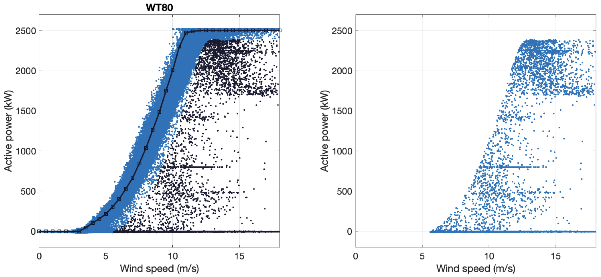
Figure 7.
On the left, in black, the anomaly points of WT80 and the power curve provided by the manufacturer. On the right, the anomalies of WT80 are isolated.

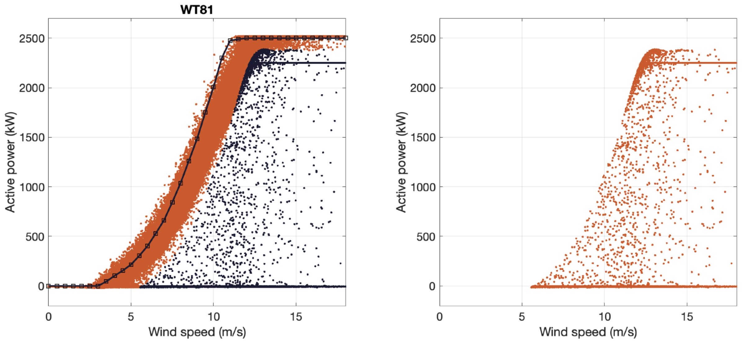
Figure 8.
On the left, in black, the anomaly points of WT81 and the power curve provided by the manufacturer. On the right, the anomalies of WT81 are isolated.
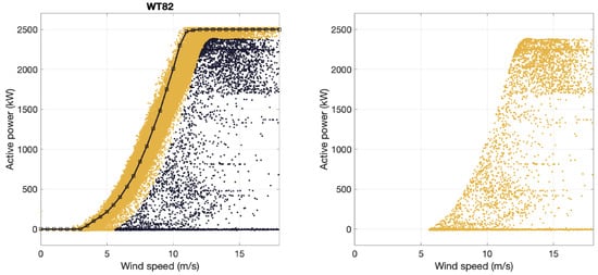
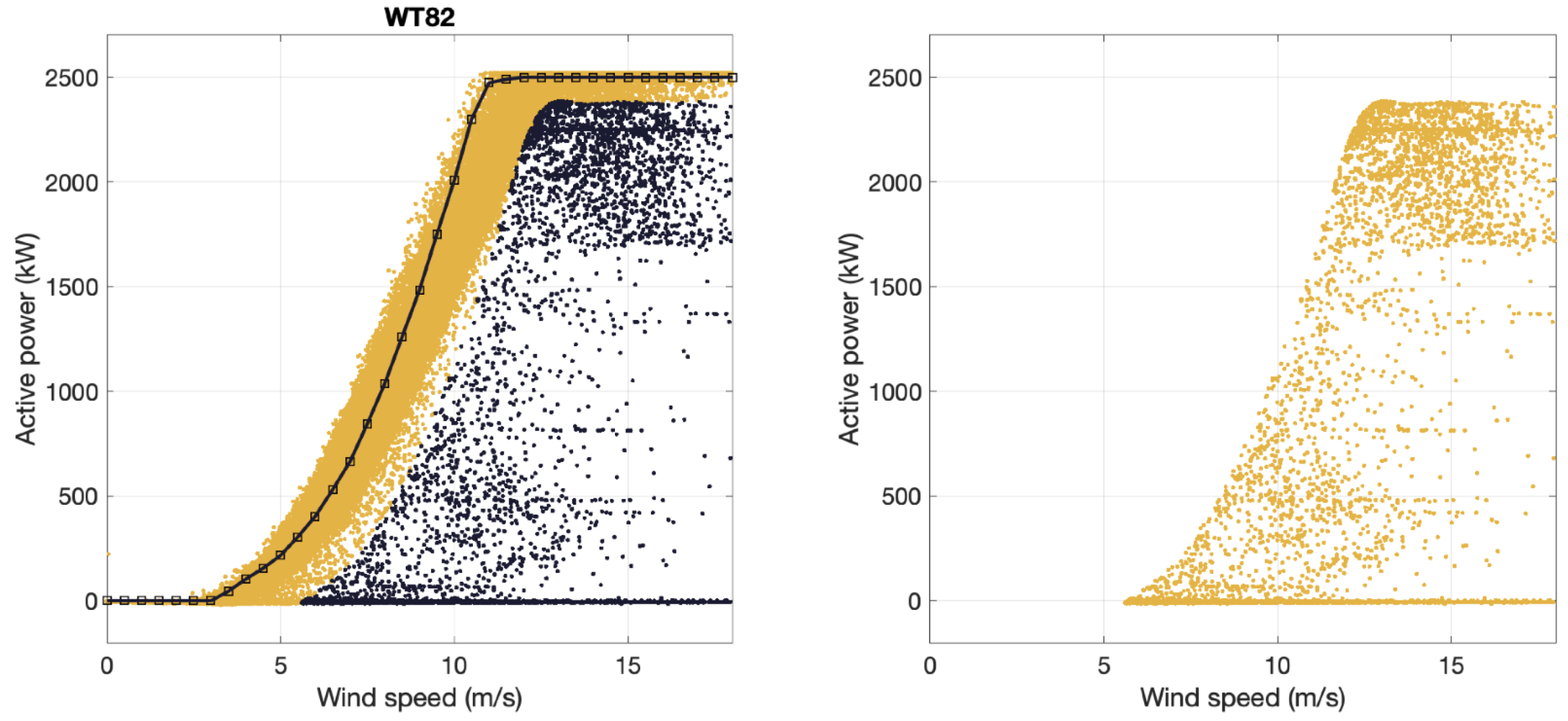
Figure 9.
On the left, in black, the anomaly points of WT82 and the power curve provided by the manufacturer. On the right, the anomalies of WT82 are isolated.
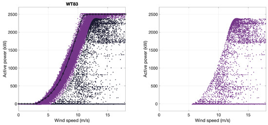
Figure 10.
On the left, in black, the anomaly points of WT83 and the power curve provided by the manufacturer. On the right, the anomalies of WT83 are isolated.
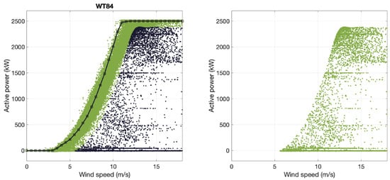
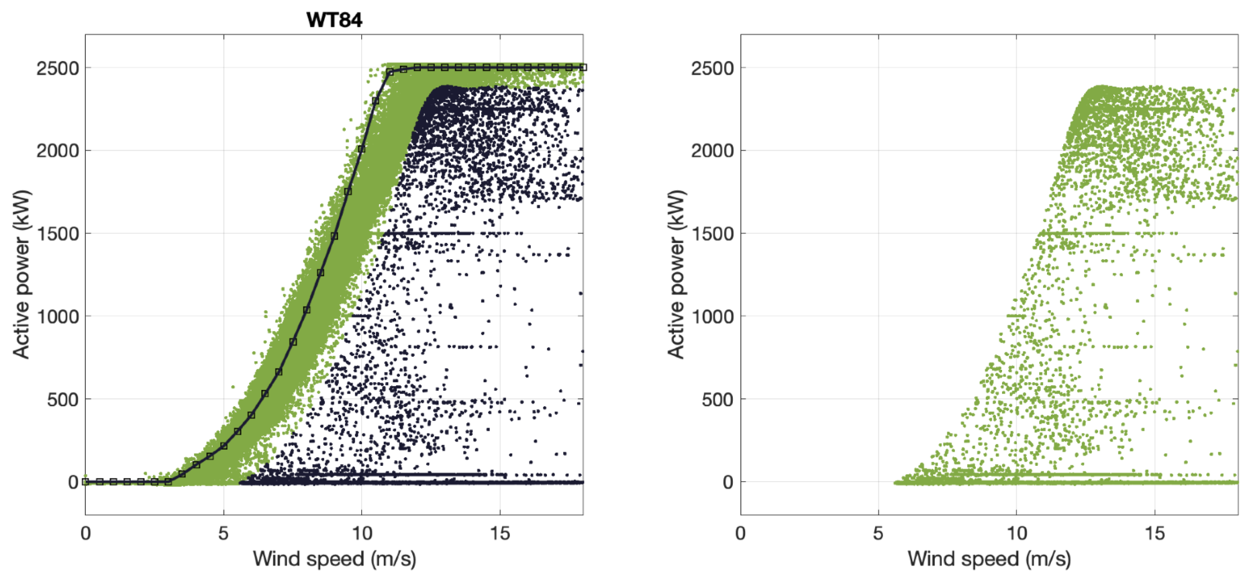
Figure 11.
On the left, in black, the anomaly points of WT84 and the power curve provided by the manufacturer. On the right, the anomalies of WT84 are isolated.
So, each figure shows the results for each of the five WTs of the WF individually. Notice that different colors identify the data of each WT. The points detected as anomalies in the left subplot are marked in black. On the color points, we present the curve, also in black, provided by the manufacturer. In the subplot on the right, we represent the points captured as anomalies in isolation.
3.2. Using the Filtered SCADA Signals to Estimate Power Curves: Training Data
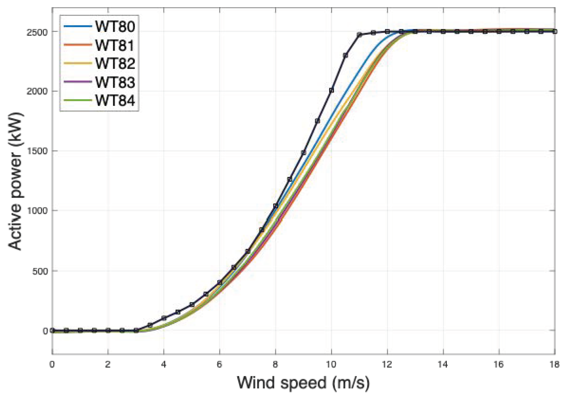
For each WT, we estimate the wind-power curve using the ANN architecture described in (3) by using 3/4 of the total available data for the training by selecting the filtered wind speeds (wnac_avg_WSpd1) as the predictor and the filtered active power (wgdc_avg_TriGri_PwrAt) as the target. For all WTs, we have used the same ANN size consisting of hidden nodes (neurons). Figure 12 shows all the estimated curves of each WT together with the power curve calculated from the data provided by the manufacturer in black indicating, in small squares, the specific points provided.
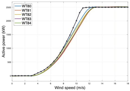
Figure 12.
Power curves of each WT estimated from the wind and power data reported by the SCADA system after removing the anomalies. The black line is the power curve provided by the manufacturer.
At this point, we notice how the estimated power-wind curves obtained from SCADA data differ from the one provided by the manufacturer, especially in the rang that goes from 8 to 12 m/s.
Comparing the estimated curves of each WT, we also notice that they are slightly different.
3.3. Using the Filtered SCADA Signals to Estimate Power Curves: Test Data
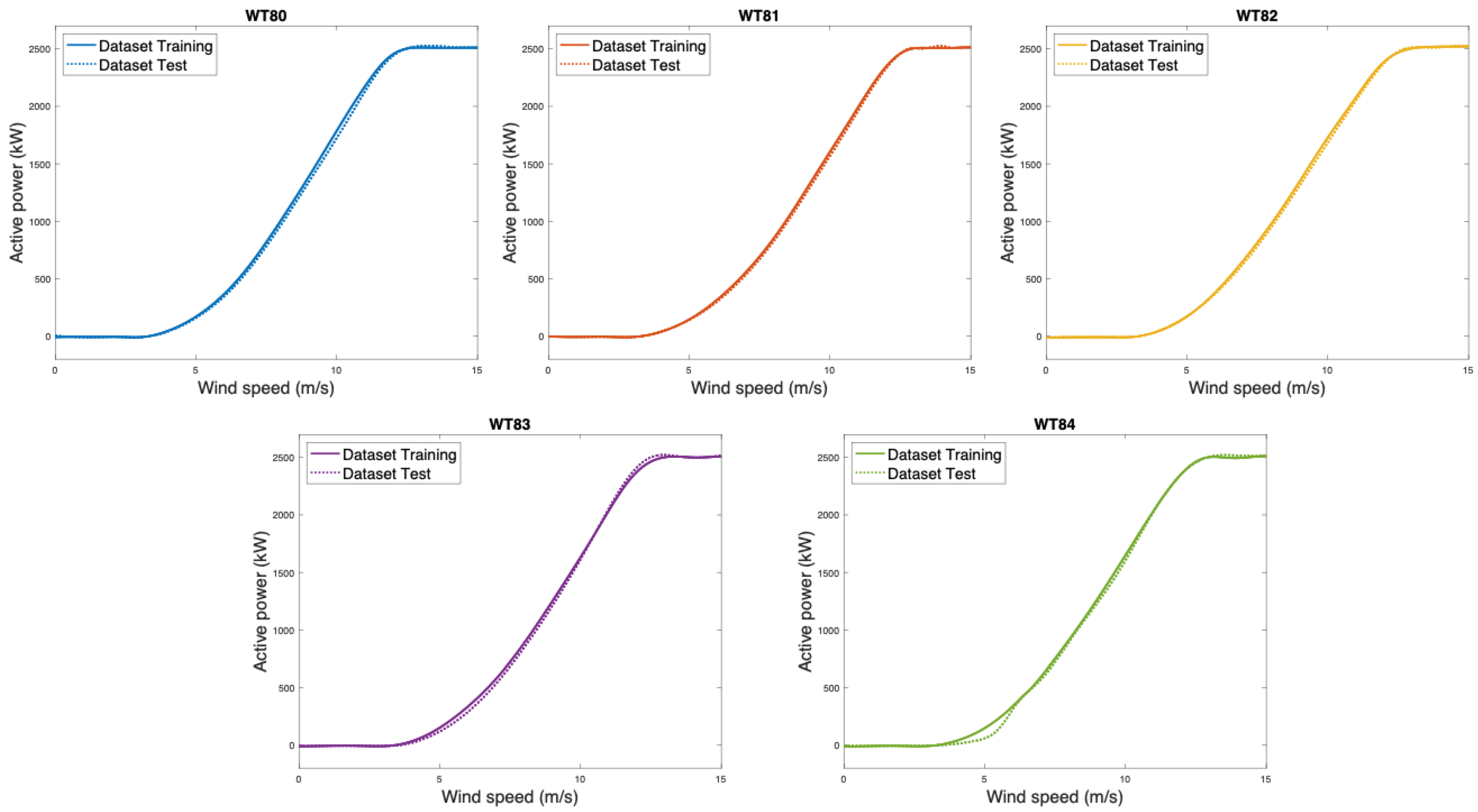
Using the same anomaly filtering and estimation method, in this section, we estimate the same curves from the last quarter of available data that we reserved for the test. Once estimated, we compare them with the curves obtained in the training part. We provide the results in Figure 13.
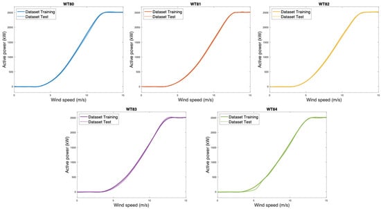
Figure 13.
Comparison between the power curves estimated with the training and the test data for each of the WTs of the WF.
It is interesting to check that the estimated power curves of each machine in the test part fit very well with those obtained using the training data. The most notable difference is the WT84 machine, which suffered a major breakdown, causing it to be stopped for a long time. In this case, we see that the differences between the curves are observed in the part of the initial start-up of the WT when little power is still generated.
3.4. Experiment 1
Next, we experiment to check whether the size of the ANNs works correctly and whether the results depend on the network size.
In the following experiment, for each WT, we use the filtered data according to the proposed filter to train a series of models of different sizes and evaluate them with the test data. We evaluate the models by calculating the RMSE of each model’s estimation error concerning the measured power. In the experiment, we evaluate ANNs with only five hidden nodes and progressively increase their hidden layer. In Table 2, we present the RMSEs obtained in the training phase, and in Table 3, the RMSEs obtained with the test data.
Table 2.
RMSE in the training (experiment 1).
Table 3.
RMSE in the test (experiment 1).
Notice that, in the test, which is the relevant part of the experiment and serves to size the network, all the ANNs evaluated work practically similarly, with the smallest configuration achieving the best result. Notice also that the magnitudes of RMSE are high, but it must be considered that the WTs are 2500 kW, and therefore, high values are handled.
3.5. Experiment 2
Once we have estimated the power curve of each WT, we have an estimate of the power curve of each WT that fits the data better than the curve determined from the points provided by the manufacturer, which has been used in the first filter. The question at this point is whether the filtering rule can be improved with the knowledge of this new curve. That is why we conduct this second experiment. We use the network of five hidden nodes to filter the row data and eliminate some points that in the improved rule may be considered anomalies, but that with the original rule may not.
In Figure 14, we show graphically, for the WT80, the power curve obtained from the ANN on the filtered data. In this experiment, for all WTs, values of and had been used, which are smaller than those used in the original filtering rule and therefore are more selective. In this figure, the points considered are shown in lighter blue, and those discarded as anomalies are shown in darker blue. With this new filtering, the previous experiment was repeated by training models of different sizes and evaluating them in the test. The results are again given in terms of the RMSE. In Table 4 for the training and in Table 5 for the test.
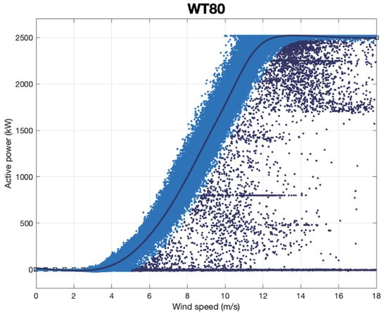
Figure 14.
Representation on the SCADA data (points in lighter blue) of the WT80 of the modification of the filtering rule by changing the manufacturer’s curve to the power curve (darker blue) estimated with an ANN of 5 hidden nodes.
Table 4.
RMSE in the training (experiment 2).
Table 5.
RMSE in the test (experiment 2).
Based on the results of this experiment, improving the filtering rule improves the results obtained in the training, but leaves the test results practically unchanged.
4. Discussion
We want to point out different aspects. In the context of this work, we understand by anomalies all those points that, due to failures in the sensors that measure the power or the wind speed or due to the starting and stopping processes of the WTs, fall in places far from the theoretical curve. Therefore, to obtain a good curve estimation, we note the need to filter anomaly data before the estimation to remove anomalies, as otherwise supervised ML-based methods also attempt to capture them into the models. So, when working with SCADA data, estimating the power curves of each WT from the data (cleaned of anomalies) is necessary, since there are significant differences from the power curve provided by the turbine manufacturer. The cause of such significant differences seems to be the nature of the SCADA data, which consists of temporal averages, in our case, of 5 minutes. Instead, the manufacturer’s values model instantaneous relations of wind and power.
In this work, we use a filtering rule that depends on the choice of and values, which can slightly determine the estimates of the curves in the regions where the curve meets the flat areas. In any case, what is vital is to consider the same rule in both the training and test phases to clean anomalies in the same way. This rule can be refined by changing the estimate of the curve provided by the manufacturer, , to the estimate of the curve measured in each WT. As noted in our work, we have kept a general rule for all WTs.
Once the estimates are made, we see that, despite presenting significant similarities, each WT has its particular curve. In this sense, it is also interesting to see that, for each WT, the estimates made with the training and test data are highly similar for all the WTs that work correctly and for the one we know has a failure in the test part, the WT84, the malfunction is captured in its curve.
The curves (to be precise, the points provided by the manufacturer) have been obtained according to a measurement protocol that is very clearly defined to be comparable between WTs from different manufacturers. Taking measurements under these conditions is expensive, so the manufacturer only provides points every 0.5 m/s. We understand, therefore, that the measurements supplied by the manufacturer are exact. In working conditions, things change slightly. First, of all, environmental conditions are continuously evolving. For example, it is known that air turbulence affects the generation conditions or that sometimes the orientation of the blades is not optimal either. These phenomena, in itself, cause observable differences between WTs of the same WF. However, one of the most significant things in this context is that the estimates are made from data provided by the SCADA system. Apart from the fact that the sensors are subject to noise, what is also very relevant is that these data are obtained from temporal averages of usually 10 min (although, in our case, they are 5 min). Temporal averages combined with wind variations in this time interval explain these differences between the estimated and manufacturer curves.
5. Conclusions
Since the malfunction of WTs directly impacts their power production capacity, characterizing the relationship between wind and power has attracted much interest. This dependence, however, is complex and non-linear since factors of a very varied nature (mechanical, electromagnetic, aerodynamic, control systems, etc.) are involved. One powerful way to express this relationship is through the wind-power curve. From the result of this work, after analyzing five WTs of a small WF, we note, after the estimation of their power curves from SCADA data, that:
- Estimated curves substantially differ from the curve that one can deduce from the data provided by the manufacturer.
- Given that the locations of the WTs are not identical, the environmental conditions of each turbine are also slightly different. Consequently, the estimated curves for each WT reflect such differences and have slight differences.
- Once the curve of one WT is determined from the training data, it is reproduced very accurately when re-estimated from the test data.
- The anomaly filtering methodology introduced permits consistently estimating the power curves using simple ANNs.
- When there is a problem in one of the WTs, such is the case of the WT84, where a fault is documented at one point in the test phase, the problem becomes visible in its power curve when estimated by test data.
Author Contributions
Conceptualization, P.M.-P. and M.S.-S.; Methodology, P.M.-P.; Software, P.M.-P., J.Á.H. and M.S.-S.; Validation, P.M.-P.; Investigation, P.M.-P., J.Á.H. and M.S.-S.; Resources, J.S.-C.; Writing—original draft, P.M.-P. and M.S.-S.; Visualization, J.Á.H.; Supervision, P.M.-P. and J.S.-C.; Project administration, J.S.-C. All authors have read and agreed to the published version of the manuscript.
Funding
This research was supported by the Ministerio de Ciencia e Innovación of the Spanish Government (ref: PID2020-120314RB-I00/AEI/10.13039/501100011033).
Institutional Review Board Statement
Not applicable.
Informed Consent Statement
Not applicable.
Data Availability Statement
The data can be extracted from the freely available database at: https://github.com/alecuba16/fuhrlander (accessed on 15 February 2024).
Acknowledgments
The author would like to thank the Smartive company (https://gust.com/companies/smartive (accessed 13 March 2024)) for providing the data used in the experimental part.
Conflicts of Interest
The authors declare no conflicts of interest.
Abbreviations
The following abbreviations are used in this manuscript:
| ANFIS | Adaptive network fuzzy inference system |
| ANN | Artificial neural network |
| GP | Gaussian Process |
| IQR | Interquartile range |
| LSE | Least-square estimate |
| LSOM | Linear Self-organized map |
| RMSE | Root mean squared error |
| SCADA | Supervisory control and data acquisition |
| SOM | Self organized map |
| WF | Wind farm |
| WT | Wind turbine |
| WT80 | Wind turbine 80 |
| WT81 | Wind turbine 81 |
| WT82 | Wind turbine 82 |
| WT83 | Wind turbine 83 |
| WT84 | Wind turbine 84 |
References
- Yang, W.; Court, R.; Jiang, J. Wind turbine condition monitoring by the approach of SCADA data analysis. Renew. Energy 2013, 53, 365–376. [Google Scholar] [CrossRef]
- Sohoni, V.; Gupta, S.; Nema, R. A critical review on wind turbine power curve modelling techniques and their applications in wind based energy systems. J. Energy 2016, 2016, 8519785. [Google Scholar] [CrossRef]
- Wang, Y.; Hu, Q.; Li, L.; Foley, A.M.; Srinivasan, D. Approaches to wind power curve modeling: A review and discussion. Renew. Sustain. Energy Rev. 2019, 116, 109422. [Google Scholar] [CrossRef]
- Woebbeking, M. IEC TS 61400-22 (First Revision of IEC WT 01). Citeseer 2008, 22, 1–11. [Google Scholar]
- Al-Quraan, A.; Al-Masri, H.; Al-Mahmodi, M.; Radaideh, A. Power curve modelling of wind turbines-A comparison study. IET Renew. Power Gener. 2022, 16, 362–374. [Google Scholar] [CrossRef]
- Bandi, M.M.; Apt, J. Variability of the wind turbine power curve. Appl. Sci. 2016, 6, 262. [Google Scholar] [CrossRef]
- Lydia, M.; Selvakumar, A.I.; Kumar, S.S.; Kumar, G.E.P. Advanced algorithms for wind turbine power curve modeling. IEEE Trans. Sustain. Energy 2013, 4, 827–835. [Google Scholar] [CrossRef]
- Wang, S.; Huang, Y.; Li, L.; Liu, C. Wind turbines abnormality detection through analysis of wind farm power curves. Measurement 2016, 93, 178–188. [Google Scholar] [CrossRef]
- Moreno, S.R.; Coelho, L.d.S.; Ayala, H.V.; Mariani, V.C. Wind turbines anomaly detection based on power curves and ensemble learning. IET Renew. Power Gener. 2020, 14, 4086–4093. [Google Scholar] [CrossRef]
- Morrison, R.; Liu, X.; Lin, Z. Anomaly detection in wind turbine SCADA data for power curve cleaning. Renew. Energy 2022, 184, 473–486. [Google Scholar] [CrossRef]
- Pandit, R.K.; Infield, D.; Kolios, A. Comparison of advanced non-parametric models for wind turbine power curves. IET Renew. Power Gener. 2019, 13, 1503–1510. [Google Scholar] [CrossRef]
- Li, S.; Wunsch, D.C.; O’Hair, E.A.; Giesselmann, M.G. Using neural networks to estimate wind turbine power generation. IEEE Trans. Energy Convers. 2001, 16, 276–282. [Google Scholar]
- Jang, J.S. ANFIS: Adaptive-network-based fuzzy inference system. IEEE Trans. Syst. Man Cybern. 1993, 23, 665–685. [Google Scholar] [CrossRef]
- Karaboga, D.; Kaya, E. Adaptive network based fuzzy inference system (ANFIS) training approaches: A comprehensive survey. Artif. Intell. Rev. 2019, 52, 2263–2293. [Google Scholar] [CrossRef]
- Raj, M.M.; Alexander, M.; Lydia, M. Modeling of wind turbine power curve. In Proceedings of the ISGT2011-India, Kollam, India, 1–3 December 2011; IEEE: Piscataway, NJ, USA, 2011; pp. 144–148. [Google Scholar]
- Ouyang, T.; Kusiak, A.; He, Y. Modeling wind-turbine power curve: A data partitioning and mining approach. Renew. Energy 2017, 102, 1–8. [Google Scholar] [CrossRef]
- Stephen, B.; Galloway, S.J.; McMillan, D.; Hill, D.C.; Infield, D.G. A copula model of wind turbine performance. IEEE Trans. Power Syst. 2010, 26, 965–966. [Google Scholar] [CrossRef]
- Astolfi, D.; Castellani, F.; Lombardi, A.; Terzi, L. Multivariate SCADA data analysis methods for real-world wind turbine power curve monitoring. Energies 2021, 14, 1105. [Google Scholar] [CrossRef]
- Pandit, R.; Kolios, A. SCADA data-based support vector machine wind turbine power curve uncertainty estimation and its comparative studies. Appl. Sci. 2020, 10, 8685. [Google Scholar] [CrossRef]
- Wang, Y.; Duan, X.; Zou, R.; Zhang, F.; Li, Y.; Hu, Q. A novel data-driven deep learning approach for wind turbine power curve modeling. Energy 2023, 270, 126908. [Google Scholar] [CrossRef]
- Letzgus, S.; Müller, K.R. An explainable AI framework for robust and transparent data-driven wind turbine power curve models. Energy AI 2024, 15, 100328. [Google Scholar] [CrossRef]
- Mclean, J.H.; Jones, M.R.; O’Connell, B.J.; Maguire, E.; Rogers, T.J. Physically meaningful uncertainty quantification in probabilistic wind turbine power curve models as a damage-sensitive feature. Struct. Health Monit. 2023, 22, 3623–3636. [Google Scholar] [CrossRef]
- Saint-Drenan, Y.M.; Besseau, R.; Jansen, M.; Staffell, I.; Troccoli, A.; Dubus, L.; Schmidt, J.; Gruber, K.; Simões, S.G.; Heier, S. A parametric model for wind turbine power curves incorporating environmental conditions. Renew. Energy 2020, 157, 754–768. [Google Scholar] [CrossRef]
- Bilendo, F.; Meyer, A.; Badihi, H.; Lu, N.; Cambron, P.; Jiang, B. Applications and modeling techniques of wind turbine power curve for wind farms—A review. Energies 2022, 16, 180. [Google Scholar] [CrossRef]
- Giebel, G.; Gehrke, O.; McGugan, M.; Borum, K. Common access to wind turbine data for condition monitoring the IEC 61400-25 family of standards. In Proceedings of the 27th Risø International Symposium on Materials Science: Polymer Composite Materials for Wind Power Turbines, Roskilde, Denmark, 4–7 September 2006. [Google Scholar]


Disclaimer/Publisher’s Note: The statements, opinions and data contained in all publications are solely those of the individual author(s) and contributor(s) and not of MDPI and/or the editor(s). MDPI and/or the editor(s) disclaim responsibility for any injury to people or property resulting from any ideas, methods, instructions or products referred to in the content. |
© 2024 by the authors. Licensee MDPI, Basel, Switzerland. This article is an open access article distributed under the terms and conditions of the Creative Commons Attribution (CC BY) license (https://creativecommons.org/licenses/by/4.0/).