A Wavelet Extraction Method of Attenuation Media for Direct Acoustic Impedance Inversion in Depth Domain

Abstract

The seismic image produced by pre-stack depth migration is more accurate and has clearer geological significance than the time image. However, the waveform of the depth-domain seismic image is affected not only by depth-dependent velocity variation but also by media attenuation, resulting in strong spectral variation of depth-domain seismic data. Therefore, depth-domain seismic inversion is still challenging. We propose a wavelet extraction method of attenuation media based on the generalized seismic wavelet, to address this issue. Then, the estimated depth-domain wavelets were applied to the direct acoustic impedance inversion. First, we investigated the effect of attenuation media on depth-domain source wavelets and derived an analytical formula for the depth-domain wavelets of attenuation media. Next, the time-domain generalized seismic wavelet was extended to the depth domain, which was utilized to study the feasibility of using the generalized seismic wavelet to characterize the seismic wavelet of the depth-domain attenuation media. Based on the orthogonal matching pursuit, we propose a method to extract the depth-domain generalized seismic wavelet directly from depth-domain seismic data. Finally, we applied this method to the depth-domain direct acoustic impedance inversion of a 3D field data example. Tests on the synthetic and 3D field datasets show that the proposed method can correctly extract the depth-domain seismic wavelet of attenuation media and attain direct inversion of the depth-domain acoustic impedance with high accuracy. Therefore, our method is effective and has robust potential in reservoir characterization, fluid prediction, and attribute extraction in the depth domain.

1. Introduction

When the velocity of the exploration area changes laterally, or the structure tends to be complex, the results of pre-stack depth migration (PSDM) are more accurate and have clearer geological significance than those of time migration [1,2,3,4]. The reason is that PSDM treats the velocity model as a single physical space and adopts a ray path accurately calculated from the imaging point to the ground through ray tracing. With the improved imaging quality of complex structures, the demand for seismic interpretation and reservoir prediction of PSDM results has gradually increased [5]. However, due to the strong spectral variation of PSDM data from shallow to deep, the methods of depth-domain direct interpretation and inversion are still in the exploration stage [6]. The fundamental reason for this strong spectral variation is that the depth-domain seismic wavelet will stretch or compress with the increase or decrease of the medium velocity, which is depth-dependent and changes with the depth. Therefore, the seismic wavelet does not have “depth invariance” in the depth domain, so the traditional convolutional model cannot be used to synthesize the depth-domain seismograms, and then the time-domain matured inversion method based on the convolutional model cannot be directly applied to the PSDM results. For consistency, we refer to non-stationarity as a feature of strong spectral variation and depth-domain seismic data as seismic images obtained by PSDM in this paper. Therefore, how to deal with this non-stationarity to achieve high-precision reservoir prediction represents an urgent geophysical problem.

Geophysicists have made many efforts to achieve depth-domain seismic inversion, which can be divided into three categories according to how they deal with non-stationarity. The first category of methods does not consider non-stationarity and treats depth-domain seismic data like time-domain seismic data. Typical approaches for this category include deep learning [7,8,9] and seismic waveform indicator inversion [10,11]. Deep learning trains a nonlinear mapping between well logs and well bypass seismic traces. Then the trained model is used to invert seismic traces at non-well positions. However, deep learning is data-driven and does not need any deterministic operator, so it has no explicit geophysical significance. Seismic waveform indicator inversion builds the initial geologic model based on seismic waveform similarity and the spatial distance between wells, and the direct inversion is carried out on depth-domain seismic data constrained by the Bayesian framework. In addition, Meza (2021) proposed a workflow for depth-domain colored inversion implemented with commercial software [12]. Because the accuracy for the first category of methods depends on the trained model, it has poor generalization performance on other depth-domain datasets.

The second category of methods, domain conversion, avoids the non-stationarity of depth-domain seismic data. It converts the depth-domain seismic data to other domains. And the matured methods in other domains have been used to carry out inversion before returning the inversion results to the depth domain. Examples of this include depth-time-depth conversion [13] and pseudo-depth conversion [14]. The depth–time-depth conversion converts seismic data between the depth and time domains using the time-depth relation [13], and the pseudo-depth conversion converts seismic data between the depth and pseudo-depth domains using both constant velocity substitution and pseudo-depth–depth relations [14]. Building on the pseudo-depth conversion, Singh (2012) and Jiang et al. (2019) developed deterministic seismic inversion workflows for rock properties [15,16]. Sun et al. (2018) used pseudo-depth conversion to invert depth-domain fluid factors [17]. In addition, Zhang et al. (2018) extracted the wavelet from depth-domain seismic data using pseudo-depth conversion and the Gibbs sampling algorithm [18]. Moreover, according to the pseudo-depth conversion, Zhang et al. (2022) searched for the wavelet that minimizes the residual difference between the synthetic record and the field data as the estimated constant wavelet in the pseudo-depth domain [19]. In short, domain conversion is time-consuming and introduces additional uncertainty to the geophysical workflow [20]. To reduce the accumulation of resampling errors caused by repeated domain conversion, Cai et al. (2022) derived an analytic formula for the depth-domain forward process from the time-domain wavelet and the depth-domain model and attained direct acoustic impedance (AI) by the least-squares method in the depth domain [2].

The last group of methods uses depth-domain seismic wavelets to accommodate the non-stationarity of depth-domain seismic data. And then it directly carries out seismic inversion in the depth domain. The approaches used for estimating depth-domain seismic wavelets mainly include point spread functions [21,22] and depth-wavenumber spectral decomposition [20,23,24]. Fletcher et al. (2012, 2016) replaced the 1D wavelet in conventional time-depth inversion with the point spread functions of depth imaging processing, attaining direct seismic inversion in the depth domain [21,22]. Then this idea was applied to complex subsalt environments [25,26,27,28], depth-domain Q compensation [29], depth-domain deghosting [30], pre-stack depth-domain elastic inversion [31,32,33], 4D inversion in the depth domain [34], and enhanced quantitative interpretation [35]. However, solving the point spread function requires a long computation time and large storage space, and the accuracy of the solution is highly dependent on the accuracy of the built depth-domain velocity model. Zhang and Deng (2018) performed depth-wavenumber spectral decomposition on the depth-domain seismic data and estimated depth-variant wavelets from the depth-wavenumber spectrum [23]. They could then carry out the inversion of the depth-domain seismic data directly through a non-stationary convolutional model. Based on this idea, Sengupta et al. (2021) also extracted depth- and angular-variant wavelets to predict depth-domain elastic parameters through linear Bayesian inversion [20]. The spectral decomposition method avoids error accumulation caused by repeated domain conversion and makes full use of the high-frequency information of logging data, which is conducive to the prediction of thin reservoirs. However, the extracted depth-variant wavelets based on the spectral decomposition method may change too sharply with the depth, affecting the accuracy of inversion results. In brief, the last group of methods mainly addresses the issues of depth-domain wavelet extraction and establishing a convolutional model for inversion.

In summary, the optimal approach uses depth-domain wavelets to characterize the non-stationarity of depth-domain seismic data. This enables direct seismic inversion based on the non-stationary convolutional model in the depth domain. However, these depth-domain seismic wavelet extraction methods do not consider attenuation. Amplitude decrease and frequency dispersion occur when the source wavelet propagates in the actual medium, and the degree of variation is related to the propagation distance and attenuation strength. The generalized seismic wavelet is a compact and flexible model, which describes the actual seismic wavelet well. The generalized seismic wavelet is defined by the fractional derivative and reference frequency. The fractional derivative controls the sidelobe and phase of the wavelet, and the reference frequency controls the width of the wavelet. The Ricker wavelet is a particular case where the fractional derivative of the generalized seismic wavelet is equal to 2. A method for estimating the time-domain generalized seismic wavelet is spectral fitting [36]. The key idea involves estimating the fractional derivative and reference frequency from the power spectrum of time-domain seismic data, which are fitted with a Gaussian function. Then, these parameters are used to construct the generalized seismic wavelet. However, the spectral fitting method assumes that the power spectra of seismic data are unimodal and change slowly. Nevertheless, in practical applications, the seismic power spectrum is usually multi-modal. It changes violently, and it is not always possible to find a suitable Gaussian function to fit the seismic power spectrum. Therefore, a separate parameter estimation (SPE) method has been proposed to estimate the optimal fractional derivative and reference frequency in the pseudo-depth domain [19]. However, the pseudo-depth-domain generalized seismic wavelet estimated by the SPE method is stationary, which is not suitable for areas with drastic changes in geological structures.

Inspired by the research of the scholars mentioned above, we propose a method to extract depth-domain wavelets based on the generalized seismic wavelet model, which not only accommodates the non-stationarity of depth-domain seismic data but also considers the influence of media attenuation. Furthermore, we apply this method to the direct inversion of depth-domain AI. For convenience, this paper only considers the effect of attenuation on the waveform of the source wavelet, and the amplitude change of the source wavelet is temporarily ignored. The remainder of this article is structured as follows: First, we study the influence of media attenuation on source wavelets and derive an analytical formula for the wavelets of attenuation media in the depth domain. Then, the depth-domain synthetic record of attenuation media is obtained based on the non-stationary convolutional model. Secondly, we extend the time-domain generalized seismic wavelet to the depth domain. Then, the feasibility of using the generalized seismic wavelet to represent the depth-domain wavelet of attenuation media is studied. Next, we propose a method to extract the depth-domain generalized seismic wavelet directly from depth-domain seismic data based on the orthogonal matching pursuit (OMP) algorithm [37]. Then, we test our method with synthetic data examples for weak and strong attenuation. Finally, we apply this method to the depth-domain AI inversion of a 3D field data example. Additionally, we compare it with the pseudo-depth-domain SPE method [19] to analyze the accuracy of our method.

2. Methodology

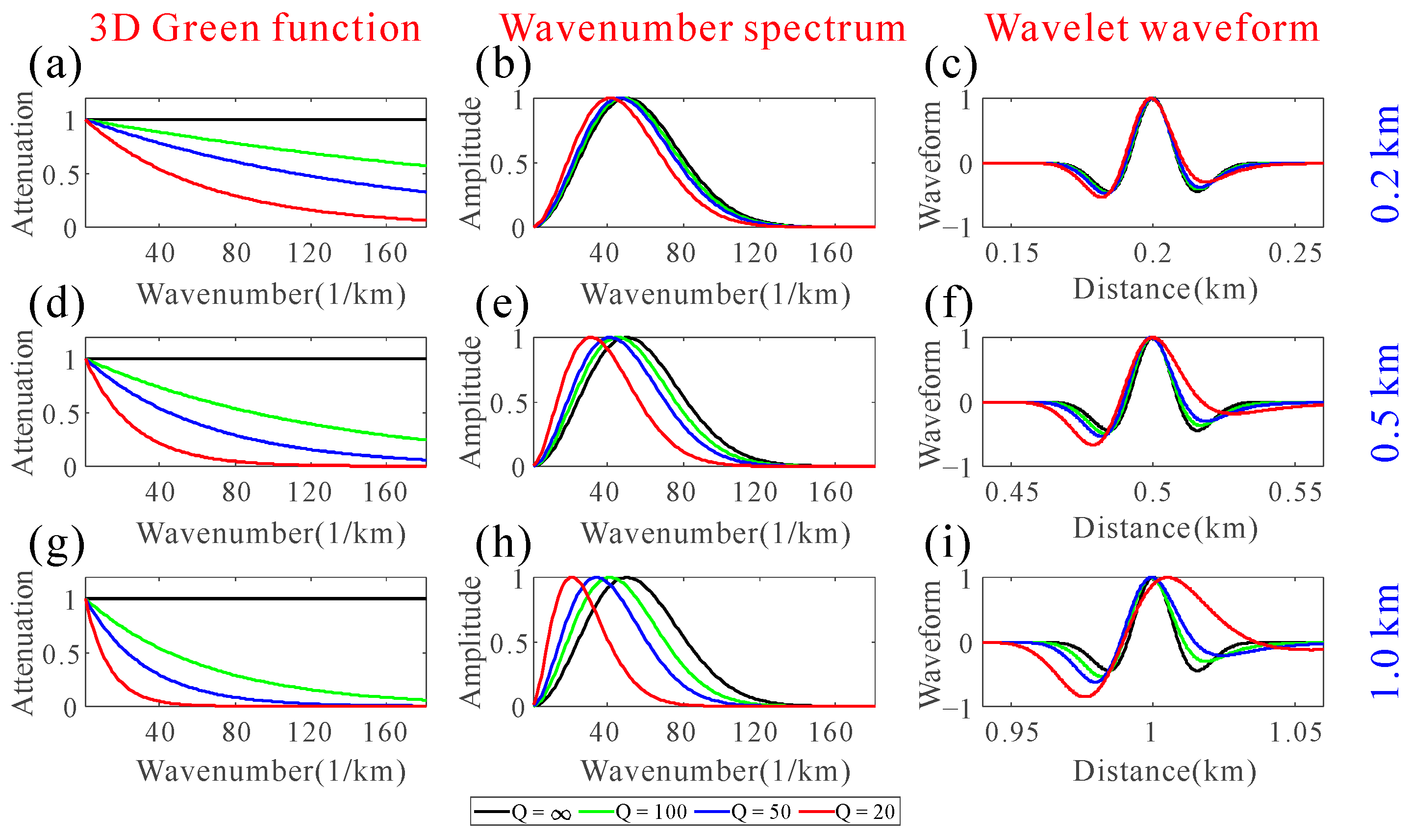
2.1. Influence of Attenuation Media on Depth-Domain Source Wavelets

In viscoelastic theory, the degree of media attenuation is usually measured by the quality factor Q, which is defined as follows:

$$Q=\frac{2\pi E}{\Delta E},$$

(1)

where E stands for the energy of a seismic wave at a reference point and $\Delta E$ is the energy loss after propagating one wavelength (or a period). The smaller the Q, the more substantial the degree of attenuation, and conversely, when Q tends to infinity, the media can be regarded as elastic. Let us start with the analytical solution of the homogeneous viscoacoustic media to investigate the influence of the attenuation media on the waveform of the source wavelet.

Assume that a homogeneous viscoacoustic medium has a velocity value of $v_0$ and a quality factor value of $Q_0$. When a time-domain source wavelet is excited at point $x_0$, its analytical solution at point x is the convolution of a source wavelet and a three-dimensional (3D) Green function in this medium. The analytical solution can be expressed as follows:

$$s\left(t\right)=f\left(t\right)\ast {\tilde{g}}_{0,3D}\left(x\left|x_0\right.,t\right),$$

(2)

where $s\left(t\right)$ is the analytical solution, $f\left(t\right)$ represents the source wavelet, and ${\tilde{g}}_{0,3D}\left(x\left|x_0\right.,t\right)$ stands for the 3D Green function. The 3D Green function is written as follows [38]:

$${\tilde{g}}_{0,3D}\left(x\left|x_0\right.,t\right)=\frac{1}{4\pi \left|x-x_0\right|}\delta \left(t-\frac{\left|x-x_0\right|}{v_0}\right),$$

(3)

where $\delta$ represents the Dirac delta function and $\left|x-x_0\right|$ denotes the distance between the source and receiver points. The result of the Fourier transform of Equation (2) can be rewritten as follows:

$$s\left(\omega \right)=F\left(\omega \right)·g_{0,3D}\left(x\left|x_0\right.,\omega \right),$$

(4)

where $s\left(\omega \right)$, $F\left(\omega \right)$, $g_{0,3D}\left(x\left|x_0\right.,\omega \right)$ denote the analytical solution, source wavelet, and 3D Green function in the frequency domain, respectively. The definition of the frequency-domain 3D Green function is as follows:

$$g_{0,3D}\left(x\left|x_0\right.,\omega \right)=\frac{e^{-i\tilde{k}\left|x-x_0\right|}}{4\pi \left|x-x_0\right|},$$

(5)

where $\tilde{k}$ is the complex wavenumber. The expression of $\tilde{k}$ is as follows [39]:

$$\tilde{k}=\frac{1}{v}\left[\omega -i\tan \left(\frac{\pi \gamma }{2}\right)\left|\omega \right|\right],$$

(6)

where v represents complex velocity and $\gamma$ denotes the attenuation factor. Their definitions are as follows:

$$\left\{\begin{array}{c}\gamma =\frac{1}{\pi }{\tan }^{-1}\left(\frac{1}{Q_0}\right)\\ v=v_0{\left|\frac{\omega }{{\omega }_0}\right|}^{\gamma }\end{array}\right.,$$

(7)

where ${\omega }_0$ is the reference angular frequency (in radians per second) and its corresponding velocity is $v_0$. Therefore, substituting $v_0$ and $Q_0$ into Equation (7) leads to the numerical complex velocity and attenuation factor. Then the numerical complex wavenumber and the 3D frequency-domain Green function can be obtained. Substituting Equation (5) and the spectrum of the source wavelet into Equation (4) yields the frequency-domain analytical solution. Moreover, the time-domain analytical solution of the wavelet can be obtained by the inverse Fourier transform of $s\left(\omega \right)$.

In the depth domain, the complex velocity should be a function of the wavenumber:

$$\left\{\begin{array}{c}\gamma =\frac{1}{\pi }{\tan }^{-1}\left(\frac{1}{Q_0}\right)\\ v=v_0{\left|\frac{k}{k_0}\right|}^{\gamma }\end{array}\right.,$$

(8)

where k is the wavenumber, $k_0$ denotes the reference angular wavenumber (in radians per meter), and its corresponding velocity is $v_0$. Therefore, the complex wavenumber for the depth domain is written as follows:

$$\tilde{k}=\frac{1}{v}\left[k-i\tan \left(\frac{\pi \gamma }{2}\right)\left|k\right|\right].$$

(9)

Substituting Equations (8) and (9) into Equation (5) yields the 3D Green function in the wavenumber domain, which can be expressed as follows:

$$g_{0,3D}\left(x\left|x_0\right.,k\right)=\frac{1}{4\pi \left|x-x_0\right|}{e}^{-i\left(\frac{1}{v_0}{\left|\frac{k_0}{k}\right|}^{\gamma }\right)\left[k-i\tan \left(\frac{\pi \gamma }{2}\right)\left|k\right|\right]\left|x-x_0\right|}.$$

(10)

Then, the wavenumber-domain analytical solution $s\left(k\right)$ is defined as follows:

$$s\left(k\right)=F\left(k\right)·g_{0,3D}\left(x\left|x_0\right.,k\right),$$

(11)

where $F\left(k\right)$ represents the wavenumber spectrum of the source wavelet. Furthermore, the depth-domain analytic solution of wavelets can be obtained by the inverse Fourier transform of $s\left(k\right)$.

It can be found from Equation (10) that the effect of the wavenumber spectrum of the source wavelet by the wavenumber-domain 3D Green function can be divided into three parts: spherical divergence caused by $1/\left(4\pi \left|x-x_0\right|\right)$, attenuation of different wavenumber components caused by $\left[k-i\tan \left(\pi \gamma /2\right)\left|k\right|\right]$, and dispersion caused by ${\left|k_0\right|}^{\gamma }/\left(v_0{\left|k\right|}^{\gamma }\right)$. This results in the attenuation of amplitude and the waveform change for the depth-domain source wavelet. The attenuation of amplitude is easy to compensate, so this paper only considers the effect of attenuation media on the source-wavelet waveform, and the change of amplitude is temporarily ignored.

The classical Ricker wavelet is commonly used as a source wavelet in seismic exploration. A standard time-domain Ricker wavelet can be written as follows [40]:

$$w\left(t\right)=\left(1-\frac{1}{2}{\omega }_p^2{\left(t-{\tau }_0\right)}^2\right)\exp \left(-\frac{1}{4}{\omega }_p^2{\left(t-{\tau }_0\right)}^2\right),$$

(12)

where ${\omega }_p$ is the most energetic or dominant angular frequency (in radians per second) and ${\tau }_0$ is the time delay. The time-depth relation links the depth and time domains, and is written as follows:

$$t=2h/v,$$

(13)

where t, h, and $v$ denote time, depth, and mean velocity, respectively. Accordingly, the relationship between wavenumber and frequency in the depth domain is as follows:

$$k=2\omega /v.$$

(14)

Substituting Equation (14) into Equation (12) yields the following:

$$w\left(h\right)=\left(1-\frac{1}{2}{k}_p^2{\left(h-l_0\right)}^2\right)\exp \left(-\frac{1}{4}{k}_p^2{\left(h-l\right)}^2\right),$$

(15)

where $k_p$ is the dominant angular wavenumber (in radians per meter), which is equal to $2{\omega }_p/v$, and $l_0$ is the depth delay. The Fourier transform of Equation (15) is expressed as follows:

$$w\left(k\right)=4\sqrt{\pi }\frac{k^2}{k_p^3}\exp \left(-\frac{k^2}{k_p^2}\right).$$

(16)

For a homogeneous viscoacoustic medium with a velocity of 2 km/s and a Q value of 20, the wavenumber-domain 3D Green function is shown as the red curve in Figure 1a, indicating that the higher the wavenumber, the greater the attenuation. When a depth-domain Ricker wavelet with a dominant wavenumber of 50 km⁻¹ propagates 0.2 km in this medium, its wavenumber spectrum and depth-domain waveform are shown as the red curves in Figure 1b,c. As shown in Figure 1c, due to the attenuation, the wavelet is no longer symmetric, the waveform widens, and the amplitude of the right sidelobe decreases. The remaining black, green, and blue curves in Figure 1a–c, respectively, show the change in the depth-domain Ricker wavelet after it propagates 0.2 km in this medium with Q values of infinity (elastic), 100, and 50. It is evident that the waveform of the wavelet becomes wider and the right sidelobe becomes more attenuated with decreased Q values. Figure 1d–i show the changes of the depth-domain Ricker wavelet after it propagates 0.5 and 1.0 km in this medium with different Q values, respectively. It can be found that the larger the distance under the same Q value, the greater the distortion of the waveform. The red curve in Figure 1h gives the wavenumber spectrum of the source wavelet after a 1.0 km propagation in this medium with a Q value of 20. It can be seen that the peak wavenumber is about 28 km⁻¹, indicating that the degree of attenuation media is about 45%. The corresponding waveform of the depth-domain wavelet is represented by the red curve in Figure 1i, where the right sidelobe is completely absorbed. Comparing the waveforms of the depth-domain wavelet in Figure 1c,f,i, it can be seen that the position of the peak is dislocated from that of the elastic due to the influence of wavenumber dispersion. The reference velocity corresponding to the reference wavenumber 50 km⁻¹ is set as 2 km/s in this test, so the component lower than the reference wavenumber propagates at a slower velocity. Conversely, the component that is higher than the reference wavenumber propagates at a faster reference velocity. Figure 2 shows the specific phase velocity of this medium under different Q values.

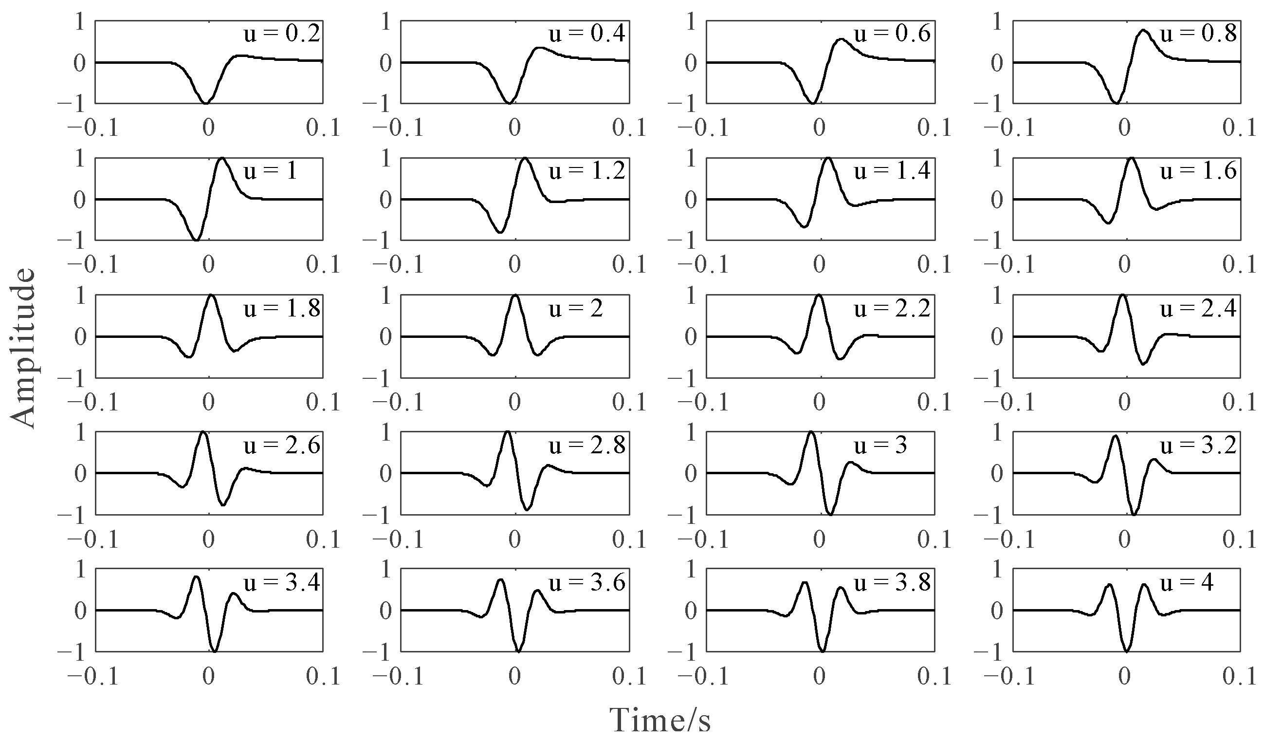
2.2. Concept of Depth-Domain Generalized Seismic Wavelet

A generalized seismic wavelet is a compact and flexible wavelet model that describes the actual seismic wavelet well. The generalized seismic wavelet is defined by the following [36]:

$$\Phi \left(\omega \left|u,{\omega }_0\right.\right)={\left(\frac{u}{2}\right)}^{-u/2}\frac{{\omega }^u}{{\omega }_0^u}\exp \left(-\frac{{\omega }^2}{{\omega }_0^2}+\frac{u}{2}\right)\exp \left(-i\omega {\tau }_0+i\pi \left(1+\frac{u}{2}\right)\right),$$

(17)

where u represents the fractional derivative, which controls the sidelobe and phase, ${\omega }_0$ denotes the reference frequency, controlling the width, and ${\tau }_0$ denotes the time delay, which controls the central position of the generalized seismic wavelet. Figure 3 shows the generalized seismic wavelet with different fractional derivatives. The reference frequency of these generalized seismic wavelets is 20 Hz, and the time delay is 0 s. It can be seen that the larger the fractional derivative, the greater the sidelobe, and the larger the phase rotation. When the fractional derivative equals 2, the generalized seismic wavelet is equivalent to the Ricker wavelet.

Substituting Equation (14) into Equation (17) yields the following:

$$\Phi \left(k\left|u,k_0\right.\right)={\left(\frac{u}{2}\right)}^{-u/2}\frac{k^u}{k_0^u}\exp \left(-\frac{k^2}{k_0^2}+\frac{u}{2}\right)\exp \left(-ik{l}_0+i\pi \left(1+\frac{u}{2}\right)\right),$$

(18)

where u represents the fractional derivative, $k_0$ denotes the reference wavenumber, controlling the width, and $l_0$ denotes the depth delay, which controls the central position of the depth-domain generalized seismic wavelet.

It is necessary to investigate the similarity between the depth-domain generalized seismic wavelet and the depth-domain attenuated wavelet before using the former to characterize the latter. Hereinafter, the term “attenuated wavelet” will refer to the wavelet of attenuation media. Figure 4 compares the depth-domain generalized seismic wavelets and attenuated wavelets shown in Figure 1, where the Q value differs between rows, and the distance varies between columns. The parameters of the depth-domain generalized seismic wavelet used in Figure 4 are shown in

Table 1. Parameter pairs of depth-domain generalized seismic wavelets (u, k₀).

	Q = ∞	Q = 100	Q = 50	Q = 20
Distance = 0.2 km	(2.00, 50.0 km−1)	(1.95, 49.0 km−1)	(1.88, 48.2 km−1)	(1.72, 25.6 km−1)
Distance = 0.5 km	(2.00, 50.0 km−1)	(1.84, 47.6 km−1)	(1.71, 45.2 km−1)	(1.42, 39.6 km−1)
Distance = 1.0 km	(2.00, 50.0 km−1)	(1.72, 45.4 km−1)	(1.51, 39.6 km−1)	(1.15, 28.6 km−1)

, where the reference wavenumbers correspond to the peak wavenumbers of the wavenumber spectrum of the depth-domain attenuated wavelets shown in Figure 1, and the fractional derivatives are obtained according to experience. Additionally, the depth delay equals the distance. As can be seen from Figure 4, the depth-domain generalized seismic wavelet and the depth-domain attenuated wavelet always have high similarity. Although the error of the two gradually increases with the decrease in the Q value or the increase in the propagation distance, the error is still tiny, even in the case of a 1.0 km propagation in the strong attenuation media with Q = 20.

Figure 5 demonstrates the Pearson correlation coefficients (PCCs) between the depth-domain generalized seismic wavelets and the depth-domain attenuated wavelets, from which, it can be seen that the similarity between the two remains high. In particular, when propagating 1.0 km in a strongly attenuated medium with Q = 20, the PCC between the depth-domain generalized seismic wavelet and the depth-domain attenuated wavelet is still greater than 98.5%. It has been proved that the depth-domain generalized seismic wavelet can be used to characterize the depth-domain wavelet of attenuation media.

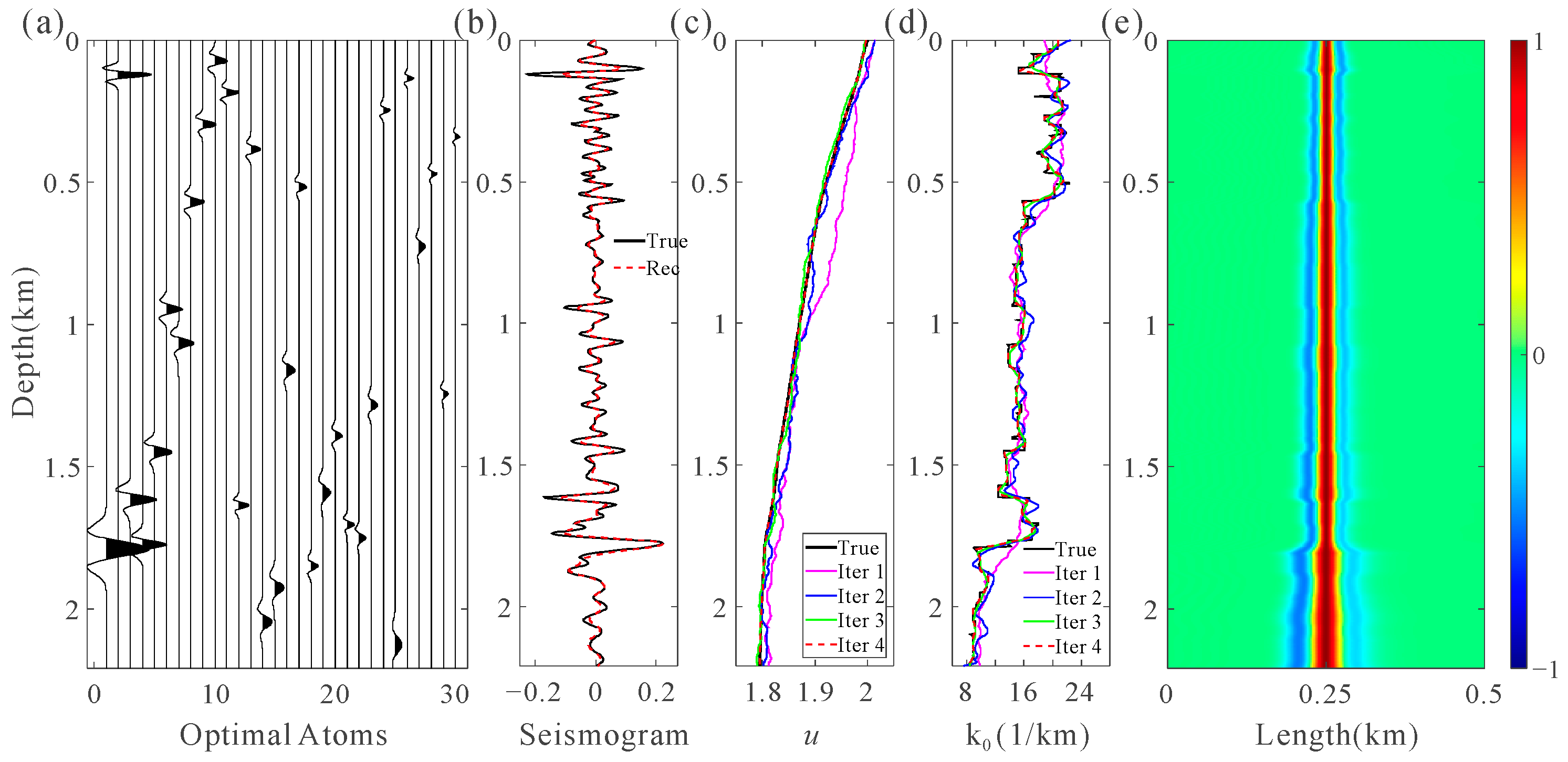
2.3. Extraction Approach of the Depth-Domain Generalized Seismic Wavelet

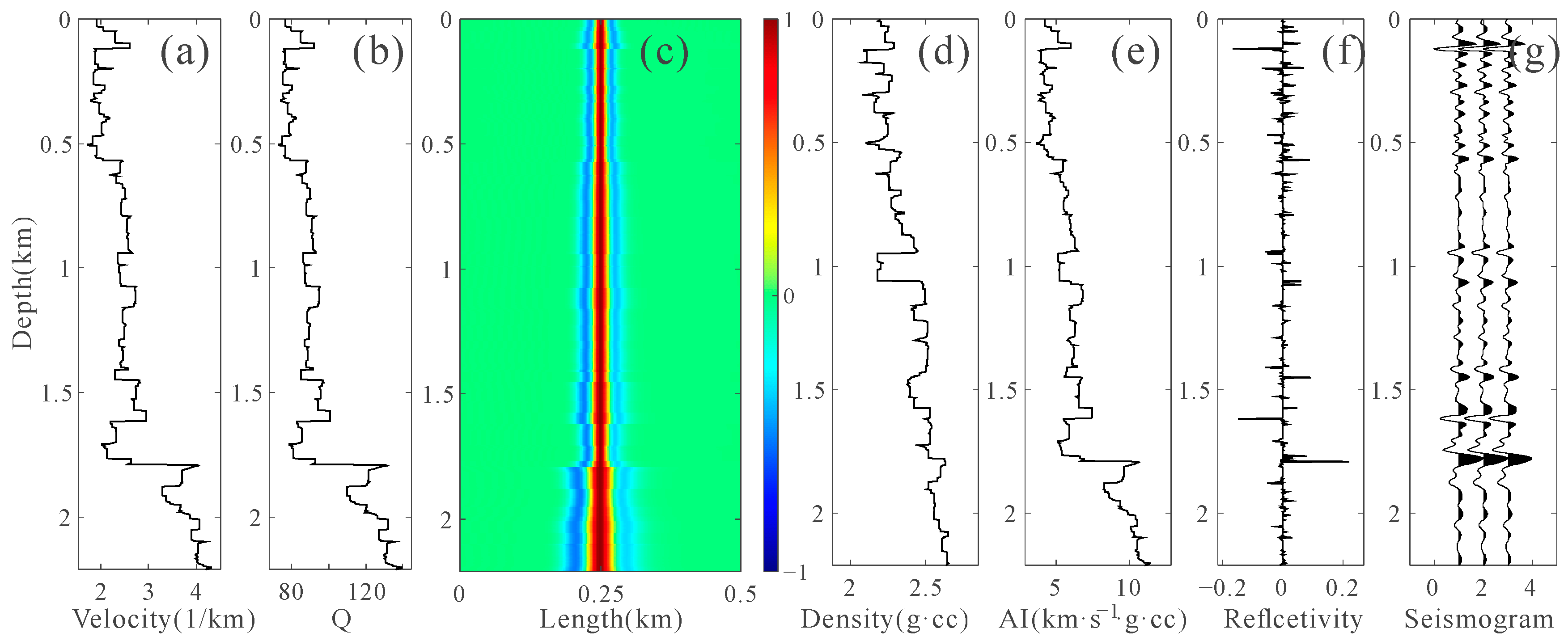
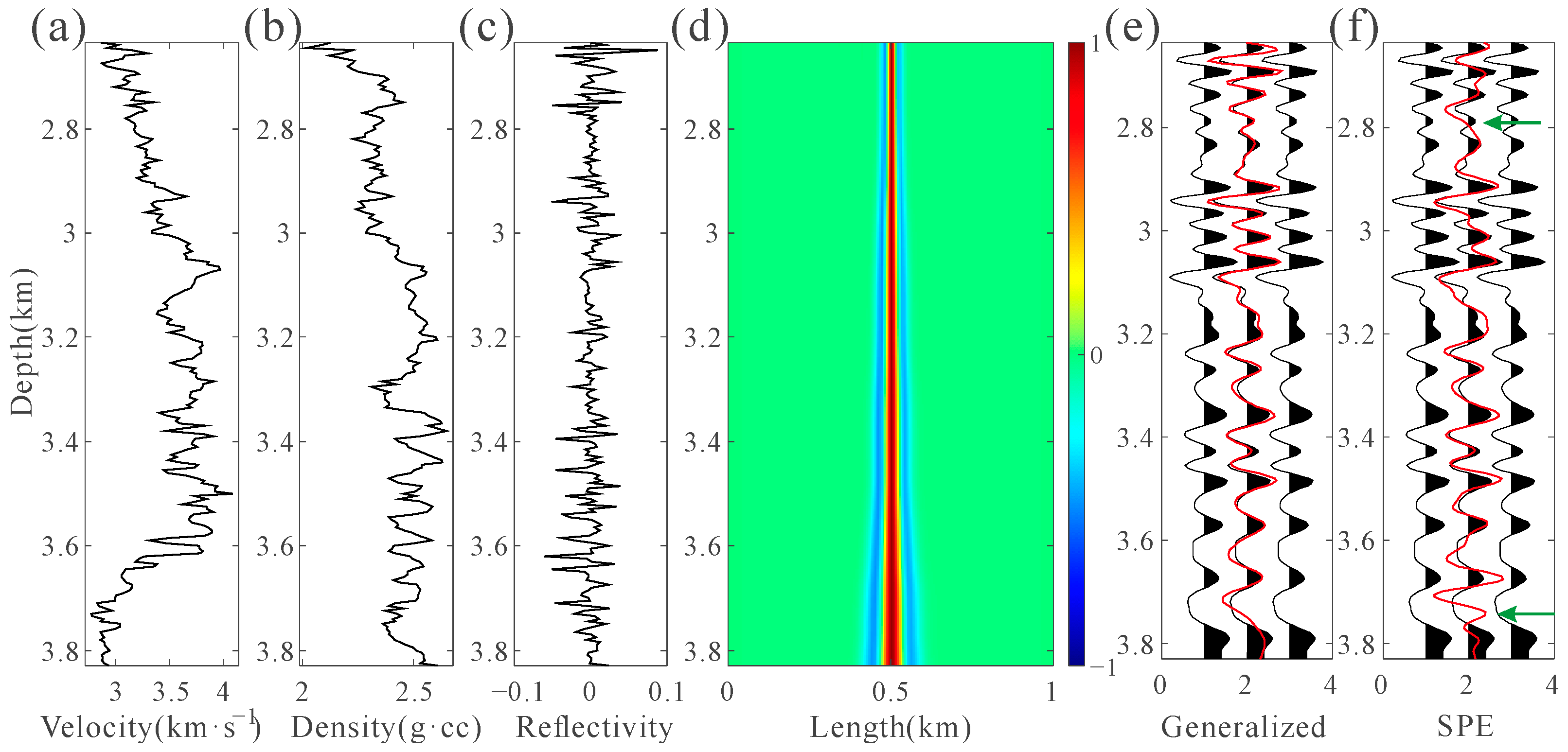
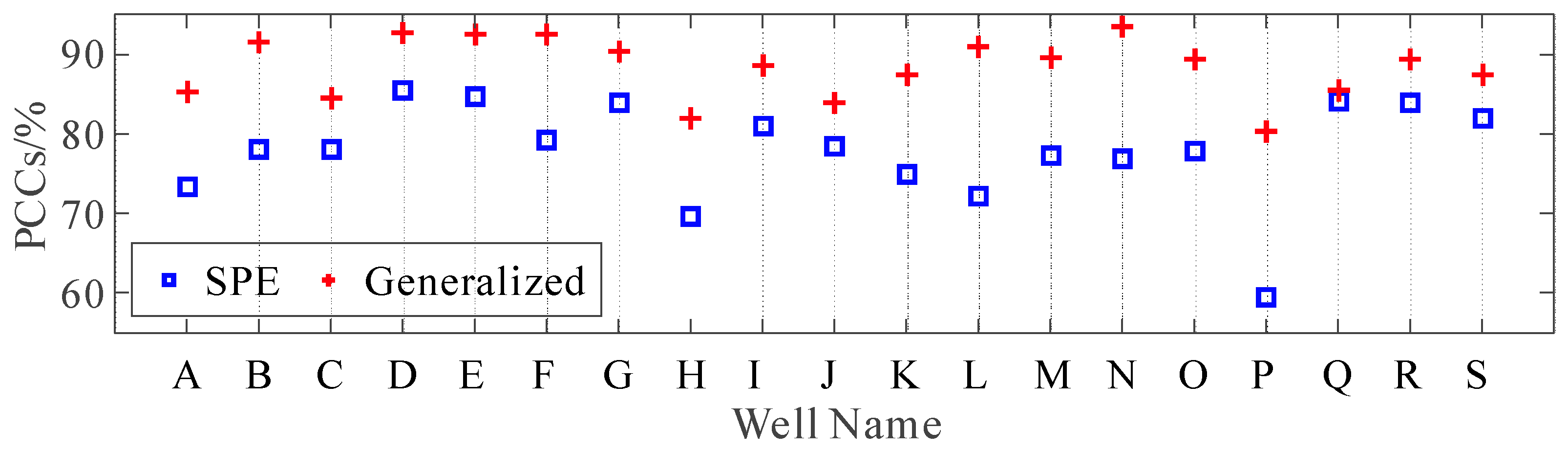
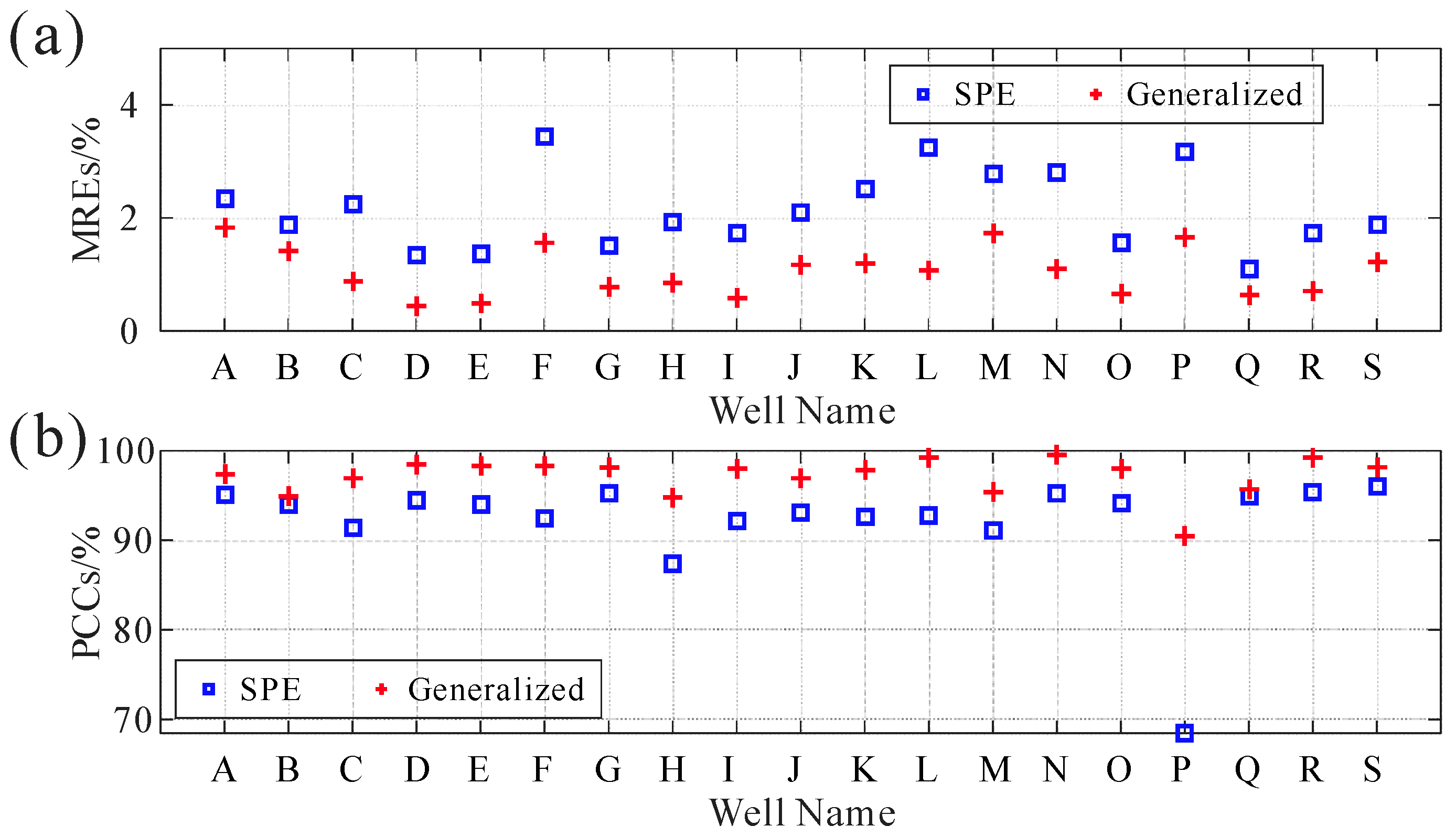
The depth-domain seismic data can be considered as the convolution of depth-domain reflectivity (reflection coefficients) and a series of depth-domain wavelets, expressed as follows [23]:

$$s\left(h\right)={\displaystyle {\int }_{-\infty }^{\infty }w\left(h-l,l\right)r\left(l\right)dl},$$

(19)

where s, w, and r represent the depth-domain seismic trace, depth-domain wavelets, and depth-domain reflectivity series, respectively. Equation (19) can be rewritten as follows:

$$\mathbf{s}=\mathbf{W}\times \mathbf{r}+\mathbf{n},$$

(20)

where s, W, r, and n denote the seismic trace vector, the wavelet kernel matrix, the reflectivity vector, and the noise vector in the depth domain, respectively.

Equation (19) indicates that the depth-domain seismic data are the summation of a series of depth-domain wavelets. Thus, the seismic data could be disassembled into the depth-domain generalized seismic wavelets series by selecting a reasonable method. OMP is a suitable method to decompose the seismic data into a batch of wavelets based on the pre-constructed overcomplete wavelet basis. Generally, the alternative wavelet basis is called the ‘wavelet atom’, and their collection—as a set—is called the ‘dictionary’ [41]. The OMP converges fast because it orthogonalizes all the atoms chosen at each iteration [37]. According to Equation (18), the overcomplete dictionary for depth-domain seismic signals, $D$, is constructed by the following:

$$D=\left\{g_{\gamma }\left(h\right)\right\}={\left\{g_{\gamma =\left(u,k_0,l_0\right)}\left(h\right)\right\}}_{\gamma \in \Gamma },$$

(21)

where $g_{\gamma }$ represents the depth-domain generalized seismic wavelet.

The implementation of OMP is iterative. The optimal depth-domain generalized seismic wavelet $g_{{\gamma }_n}$ is extracted from the overcomplete dictionary at each iteration adaptively, where n represents the n-th iteration. Before conducting OMP on the seismic trace $s\left(h\right)$, one should initialize the residuals, $R^{\left(0\right)}s=s$, and the index set, ${\Lambda }_0=\varnothing$, which is the set of optimal wavelet atoms. Then, the optimal wavelet, $g_{{\gamma }_n}\left(h\right)$, at the n-th iteration can be obtained from the following equation:

$$g_{{\gamma }_n}\left(h\right)=\arg \underset{g_{{\gamma }_n}\in D}{\max }\frac{\left|〈R^{\left(n\right)}s,g_{{\gamma }_n}〉\right|}{‖g_{{\gamma }_n}‖},$$

(22)

where $〈·,·〉$ denotes the inner product and $‖g_{{\gamma }_n}‖=\sqrt{〈g_{{\gamma }_n},g_{{\gamma }_n}〉}$ normalizes the wavelet $g_{{\gamma }_n}$. The optimal wavelet atom is added to the index set by ${\Lambda }_n=\left[{\Lambda }_{n-1},g_{{\gamma }_n}\right]$. Then, the amplitude coefficient, $a_n$, is solved by the following:

$$a_n=\arg \min ‖s-{\Lambda }_n{a}_n‖,$$

(23)

The solution to Equation (23) is as follows:

$$a_n={\left({\Lambda }_n^T{\Lambda }_n\right)}^{-1}{\Lambda }_n^{T}s,$$

(24)

where ${\Lambda }_n^T$ denotes the transpose of ${\Lambda }_n$. Finally, the residual is updated through the following equation:

$$R^{\left(n\right)}s=s-{\Lambda }_n{a}_n.$$

(25)

Equations (22)–(25) represent one complete iteration of the depth-domain generalized seismic wavelet overcomplete dictionary-based OMP (OMP-G_d) decomposition of the depth-domain seismic data. The algorithm kills when the pre-set threshold is larger than the residual error or n exceeds a pre-set maximum iteration number. The seismic trace after N iterations is written as follows:

$$s\left(h\right)={\displaystyle \sum _{n=0}^{N-1}{a}_n{g}_{{\gamma }_n}\left(h\right)}+R^{\left(N\right)}s,$$

(26)

where the minimum residual, $R^{\left(N\right)}s$, is regarded as the data noise.

After obtaining the optimal depth-domain generalized seismic wavelet atom by decomposing the seismic trace, the fractional derivative and reference wavenumber of each optimal atom are recorded, and these parameters can be arranged according to the depth and interpolated to obtain the parameters of the generalized seismic wavelets of the whole seismic trace. Therefore, the depth-domain generalized seismic wavelets are constructed with the obtained parameters. Generally, the rough dictionary leads to high computational efficiency but low accuracy. On the other hand, the fine dictionary has low computational efficiency but high accuracy of the results. Therefore, the rough dictionary with an extensive search range and interval is first established to simultaneously consider the computational efficiency and accuracy. Then, the OMP-Gd of the depth-domain seismic data is conducted to obtain a rough estimate of the parameters of the generalized seismic wavelets. After the first OMP-G_d, a finer dictionary based on the rough estimate is established. The final generalized seismic wavelets can be obtained by repeating this step. Figure 6 shows the specific workflow, where M indicates the repeated OMP-G_d number and is usually set at 3 or 4.

3. Examples

Before testing the proposed wavelet extraction method, we synthesize the depth-domain seismogram as input. For a depth-domain heterogeneous viscoacoustic model with a sampling number, N, and depth sampling interval, $\Delta h$, the wavenumber spectrum, $F_i\left(k\right)$, of the attenuated wavelet at point i can be written as follows:

$$F_i\left(k\right)=F_0\left(k\right)·\underset{j=1}{\overset{i}{{\displaystyle \Pi }}}{g}_{0,3D_j}\left(x\left|x_0\right.,k_j\right),$$

(27)

where $F_0\left(k\right)$ is the wavenumber spectrum of the source wavelet, $\Pi$ means accumulative multiplication, $g_{0,3D_j}\left(x\left|x_0\right.,k_j\right)$ represents the wavenumber-domain 3D Green function at point j, and $k_j$ denotes the wavenumber at point j, which is related to the velocity at point j. Additionally, the distance, $\left|x-x_0\right|$, equals the depth sampling interval, $\Delta h$. Therefore, the depth-domain attenuated wavelet at point i can be obtained by the inverse Fourier transform of $F_i\left(k\right)$. Substituting the depth-domain attenuated wavelets and the reflectivity into Equation (20) yields the depth-domain synthetic seismogram.

A depth-domain weak attenuation model with sampling number 885 and a depth sampling interval of 0.0025 km is presented in Figure 7, which is used to elaborate the workflow of our depth-domain generalized seismic wavelet extraction method. Figure 7a,b depict the velocity and Q, respectively. When a 20 Hz Ricker wavelet propagates through the weak attenuation model, the depth-domain attenuated wavelets computed by Equation (27) are displayed in Figure 7c. It can be seen that with increasing depth, the waveform of the attenuated wavelet is no longer symmetrical. The energy of the right sidelobe decreases, and the energy of the left sidelobe increases. Figure 7e is the AI calculated through the density shown in Figure 7d and the velocity shown in Figure 7a. Figure 7f is the reflection coefficient. Substituting the depth-domain attenuated wavelets and the reflectivity into Equation (20) yields the depth-domain synthetic seismogram, as demonstrated in Figure 7g.

Next, the proposed method extracts the depth-domain generalized seismic wavelets from the depth-domain synthetic seismogram. Figure 8a shows the overcomplete dictionary established by the depth-domain generalized seismic wavelets during the first OMP-G_d. The search range of the fractional derivative is 1.5~2.1 with an interval of 0.05, the search range of the reference wavenumber is 6~26 km⁻¹ with an interval of 1 km⁻¹, and the depth delay ranges from 0 to 2.21 km with an interval of 0.0025 km. Figure 8b shows the first 2000 atoms enlarged in Figure 8a.

The depth-domain generalized seismic wavelet extraction test of Figure 7g is demonstrated in Figure 9. Figure 9a shows the first 30 optimal depth-domain generalized seismic wavelet atoms obtained from the first OMP-G_d. The red dotted line in Figure 9b represents the reconstructed seismogram of the first OMP-G_d obtained by adding these optimal atoms, and the black solid line is the actual seismogram. It can be seen that the primary waveforms of the reconstructed seismogram match those of the real seismogram well. Figure 9c,d show the extracted fractional derivative and reference wavenumber, respectively, where the solid black line represents the reference value calculated according to the analytical wavenumber spectrum of Equation (26). The magenta, blue, and green solid lines represent the extraction results of the first, second, and third iterations of OMP-G_d, while the red dotted line is the result of the fourth OMP-G_d (the final output). It can be seen that with the increase in the number of iterations, the extracted parameters of depth-domain generalized seismic wavelets move closer to the reference values. Figure 9e shows the corresponding depth-domain generalized seismic wavelets, which are very similar to the depth-domain attenuated wavelets in Figure 7c.

We compare our method with the pseudo-depth-domain SPE method. Figure 10 shows the extraction results of the pseudo-depth-domain SPE method, where the vertical ordinate is the pseudo-depth. Figure 10a shows the pseudo-depth-domain seismogram obtained by converting the depth-domain seismogram with the depth-domain velocity model and the constant velocity value of 3 km/s into the pseudo-depth domain. Similarly, Figure 10b shows the pseudo-depth-domain reflection coefficient. Figure 10c,d show the extracted constant wavelet and the synthetic record in the pseudo-depth domain, respectively. Figure 11 displays the depth-domain synthetic records obtained by the pseudo-depth-domain SPE method and the depth-domain generalized seismic wavelet extraction method, where the former is returned to the depth domain from the result in Figure 10d. Due to the resampling in the pseudo-depth-domain conversion, the reflection coefficients are stretched or compressed. Therefore, the synthetic record of the pseudo-depth-domain SPE method poorly matches the real seismogram. As the green arrows show, it exhibits distortion and dislocation of the waveform and changes the relative energy relationship between waveforms. In contrast, the synthesized record obtained by the proposed method agrees with the actual seismogram in terms of the waveform and amplitude. The PCCs between the synthetic records and the real seismogram are 85.7% and 98.52%, respectively, showing that our method can accurately extract the depth-domain attenuated wavelets in the case of weak attenuation.

In practice, some media exhibit strong attenuation, namely small Q, such as weathering zones and deserts, etc. Therefore, based on the weak attenuation model, the value of the quality factor is reduced to build a strong attenuation model in the depth domain, as shown in Figure 12a. Also, let a 20 Hz Ricker wavelet propagate through the depth-domain strong attenuation model. The depth-domain attenuated wavelets computed through Equation (26) are displayed in Figure 12b. It can be found that with increasing depth, the energy of the right sidelobe decreases more than that of the weak attenuation model. Figure 12c demonstrates the depth-domain synthetic seismogram by convoluting the depth-domain attenuated wavelets with the reflectivity shown in Figure 7f. By comparing the seismograms in Figure 7g and Figure 12c, it is evident that the deep waveform becomes significantly wider in the case of strong attenuation, marked by the cyan dashed ellipse. Next, the proposed method extracts the depth-domain generalized seismic wavelets, as seen in Figure 12c. Figure 12d shows the estimated depth-domain generalized seismic wavelets, which are highly similar to the depth-domain attenuated wavelets in Figure 12b. Figure 12f is the estimated pseudo-depth-domain constant wavelet by the pseudo-depth SPE method. Figure 12e compares depth-domain synthetic records obtained by the two methods. Similarly, the synthetic record of the pseudo-depth-domain SPE method matches the real seismogram poorly, with distortion and dislocation of the waveform. As the green arrows show, the synthetic record has a reverse trend. The synthetic record obtained by the proposed method also agrees with the actual seismogram regarding the waveform and amplitude. The PCCs between the synthetic records and the real seismogram are 76.53% and 98.11%, respectively. Tests of the synthetic data example prove that our method can accurately extract the depth-domain attenuated wavelets in the case of attenuation media. In the next section, we will show a 3D field seismic dataset to demonstrate the effectiveness of the proposed method for direct AI inversion in the depth domain.

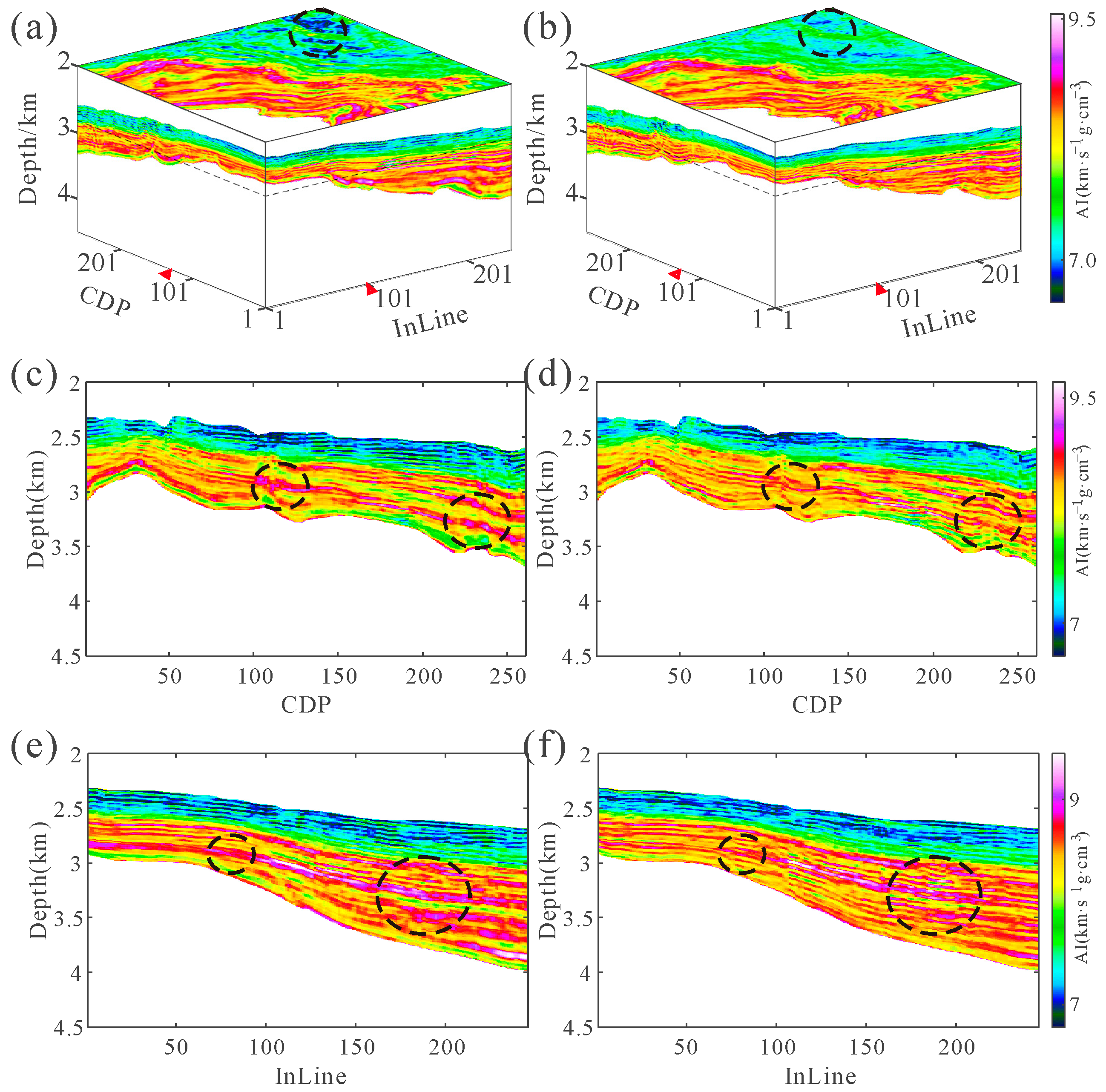
4. Inversion on a 3D Field Dataset

After extracting the depth-domain generalized seismic wavelet, it can be applied to the depth-domain AI inversion. Basis pursuit (BP) is an optimization method with an L₁ norm. Considering the sparsity of subsurface stratigraphy, the BP has been gradually applied to seismic inversion in recent years, which improves the detectability and resolution of thin layers [23,24]. Here, we use the BP inversion approach to obtain the reflectivity, and the inverted AI should be recovered by the following:

$$I_H=I_0\exp \left(2{\displaystyle \sum _{h=h_0}^H{r}_h}\right),$$

(28)

where $I_H$ is the AI at depth H and $I_0$ is the AI at the initial depth $h_0$. The initial AI model can be constructed by interpolating well-log measured AI. We also use the inversion result of the pseudo-depth-domain SPE method for comparison, which converts depth-domain seismic data to the pseudo-depth domain and performs inversion using the same BP inversion technique before converting the result back to the depth domain. We use the same depth-domain seismic data, the same initial AI model, and the same regularization parameters for the two methods. To quantify the accuracy of different inversion results, we use the mean relative error (MRE), written as follows:

$$\mathrm{MRE}=\frac{100\%}{MN}{\displaystyle \sum _{i=1}^M{\displaystyle \sum _{j=1}^N\left|\frac{{\widehat{I}}_{i,j}-I_{i,j}}{I_{i,j}}\right|}},$$

(29)

where $\widehat{I}$ is the inverted AI, and $I$ is the actual AI.

In this study, we perform inversion on a 3D depth-domain field seismic dataset from East China, as depicted in Figure 13a. The seismic data comprises 246 survey lines with a line interval of 0.025 km. Each line has 261 traces or 261 CDP, and the trace spacing is also 0.025 km. The depth ranges from 2.0 km to 4.5 km with a depth sample interval of 0.005 km. The red arrows shown in Figure 13a,b indicate the direction. In this paper, the black dotted lines indicate the actual positions of the slices in 3D figures. Take Figure 13a as an example; the slice shown at the top is a horizontal slice with a depth of 3.3km in the seismic dataset; the situation is the same for the below. Figure 13b shows the four seismic horizons of this seismic dataset. It can be seen that the terrain of this region is high in the southwest and low in the northeast, and layers 3 and 4 are gradually separated along the southwest to northeast direction. There are 19 wells in this region, as shown in Figure 13c, named wells A to Q. And the distribution of wells is relatively uniform. Figure 13d presents the initial AI model established by interpolating the well-log data along the seismic horizons.

First, our method extracts the generalized seismic wavelet parameters from the 3D depth domain seismic data, as shown in Figure 6. Figure 14a,b show the extracted fractional derivative and reference wavenumber, respectively. The fractional derivative ranges from 1.9 to 2.04, indicating that the shape of the extracted depth-domain generalized seismic wavelet, is close to the Ricker wavelet. The reference wavenumber tends to be lower with increased depth.

Next, the pseudo-depth-domain SPE method is used for comparison. The pseudo-depth-domain SPE method can estimate a constant wavelet at each well for this 3D depth-domain seismic dataset. However, only one wavelet should be used during the inversion. Therefore, after extracting the pseudo-depth domain constant wavelet from each well, it is applied to all wells to obtain the pseudo-depth domain synthetic records. The PCCs between the synthetic records and the well bypass seismograms are computed in the pseudo-depth domain. The pseudo-depth-domain constant wavelet with the highest average PCCs is the final constant wavelet output utilized for the pseudo-depth-domain inversion. Figure 15 shows the estimated pseudo-depth-domain constant wavelet at well D, which has the highest average PCCs. Figure 15a–d demonstrate the depth-domain well-log velocity, well-log density, reflectivity, and seismogram of well D, respectively. Figure 15e is the pseudo-depth-domain seismogram obtained by converting Figure 15d with velocity in Figure 15a and a constant velocity value of 3 km/s into the pseudo-depth domain. Similarly, Figure 15e shows the pseudo-depth-domain reflectivity. Figure 15f displays the extracted constant wavelet in the pseudo-depth domain.

The well-to-seismic tie at well N, which aligns the well log and seismic data with the former depth only, is displayed in Figure 16 to verify the accuracy of the extracted wavelets. Figure 16a–c display the well-log velocity, density, and reflectivity. The depth-domain generalized seismic wavelets at the location of well N are demonstrated in Figure 16d, which are constructed using the parameters shown in Figure 14. Figure 16e compares the synthetic seismogram obtained by the depth-domain generalized seismic wavelets (red curve) with the well bypass seismogram (black wiggle variable area), which shows high similarity. The red curve in Figure 16f is the synthetic seismogram obtained by the pseudo-depth-domain constant wavelet, which poorly matches with the actual well bypass seismogram (black wiggle variable area) regarding the waveform and amplitude. Furthermore, the green arrow marks a reverse trend in the synthetic seismogram. The PCCs between the synthetic records and the actual well bypass seismograms are 76.93% and 93.41%, respectively. Similarly, Figure 17 shows the PCCs between the synthetic records and the actual well bypass seismograms for all wells, where the abscissa demonstrates the name of the well, and the blue square and red plus symbol represent the pseudo-depth-domain SPE method and the depth-domain generalized seismic wavelet extraction method, respectively. It can be seen that our method has high accuracy overall. The PCCs of most wells are above 90%. The accuracy of the pseudo-depth-domain SPE method is low, especially that of well P, which is even less than 60%. Therefore, it is proven that our method can accurately extract the depth-domain wavelets from the field dataset.

Figure 18a,b show the inverted AI of the pseudo-depth-domain constant wavelet and the depth-domain generalized seismic wavelets, respectively. It can be found that the AI of the horizontal slice of the former changes more sharply than that of the latter. For example, the inverted AI of Figure 18a in the black ellipse area is significantly lower than that of Figure 18b. In addition, by comparing the profiles of the two results, it can be seen that the inversion result of the depth-domain generalized seismic wavelet has better thin layer resolution and lateral continuity than that of the pseudo-depth-domain constant wavelet. To further investigate the accuracy of the two inversion results, Figure 18c,e display the InLine 101 and CDP 131 profiles of Figure 18a,d,f, and show the InLine 101 and CDP 131 profiles of Figure 18b. As can be seen from the comparison of the black ellipse region in the InLine 101 profiles, the inversion AI of the pseudo-depth-domain constant wavelet is not as continuous as the other one in the structural changes, and the formation resolution is lower. The comparison of the black ellipse region in the CDP 131 profiles also verifies this viewpoint.

Figure 19 presents the comparison between the inverted and well-log AI at wells D, H, and N, where Figure 19b,d,f are the enlarged views of the cyan box area in Figure 19a,c,e, respectively. The black curve represents well-log AI, while the blue and red curves are the inverted AIs of the pseudo-depth-domain constant wavelet and the depth-domain generalized seismic wavelets. It can be seen that the main variation trend of inversion results of the two wavelets is consistent with well-log AI. However, the deviation between the inversion results of the pseudo-depth-domain constant wavelet and the well-log AI is significant. Conversely, the inversion results of the depth-domain generalized seismic wavelets are more consistent with the well-log AI regarding variation trends and structural details, as marked by the red arrow in Figure 19. Figure 20a,b present the MREs and PCCs between the inverted and measured AI for all wells, where the abscissa also demonstrates the name of the well, and the blue square and red plus symbol also denote the pseudo-depth-domain SPE method and the depth-domain generalized seismic wavelet extraction method, respectively. It can be seen from Figure 20a that the MREs of inversion results through the proposed method are lower than those of the pseudo-depth-domain SPE method. The MREs of inversion results through the proposed method for all wells are less than 2%, and most are even less than 1%, especially the MRE at well D, which is only about 0.4%. In comparison, the MREs of inversion results by the pseudo-depth-domain SPE method are above 2% on the whole. From Figure 20b, the large PCCs of inversion results using our method indicate that the variation trend of inverted AI is close to the well-log AI. However, the PCC of inverted AI through the pseudo-depth-domain SPE method at well P is even lower than 70%. It demonstrates that there is a large deviation between the inversion results and well-log AI in detail. Therefore, the depth-domain 3D field dataset test demonstrates that the method proposed in this paper can be effectively applied to the depth-domain direct AI inversion.

5. Conclusions

Within the seismic wavelength range, the waveforms of the depth-domain seismic wavelets change when there is a structure change or fluid in the formation. And the waveforms of the depth-domain seismic wavelets are also affected by the attenuation media. In this case, using the constant wavelet to characterize the depth-domain seismic wavelets will cause a large error in the synthesized seismogram. This work proposes a wavelet extraction method of attenuation media based on the generalized seismic wavelet to address this issue. Tests of weak and strong attenuation models demonstrate that the proposed method can correctly depict the depth-domain attenuated wavelets. Therefore, our method can be effectively applied to the depth-domain well-to-seismic calibration. Moreover, the AI inversion result of a 3D field dataset shows high accuracy and fine structure because the depth-domain generalized seismic wavelets are more suitable for describing the change in seismic facies than the constant wavelet. Hence, the proposed method can be utilized effectively for depth-domain AI inversion, and it has promising potential in reservoir characterization, fluid prediction, and attribute extraction in the depth domain. In the future, this method could be extended to applications on depth-domain prestack data for inverting subsurface elastic properties.

References

1. Etgen, J.T.; Kumar, C. What really is the difference between Time and Depth Migration? A tutorial. In Proceedings of the 82nd Annual International Meeting, SEG, Expanded Abstracts, Salt Lake City, UT, USA, 6–11 October 2012; pp. 1–5. [Google Scholar] [CrossRef]
2. Cai, R.; Sun, C.; Li, S. A strategy for acoustic impedance direct inversion in depth domain. In Proceedings of the Second International Meeting for Applied Geoscience & Energy, SEG, Expanded Abstracts, Houston, TA, USA, 28 August–2 September 2022; pp. 228–232. [Google Scholar] [CrossRef]
3. Li, B.; Sun, M.; Xiang, C.; Bai, Y. Least-Squares Reverse Time Migration in Imaging Domain Based on Global Space-Varying Deconvolution. Appl. Sci. 2022, 12, 2361. [Google Scholar] [CrossRef]
4. Liang, H.; Zhang, H.; Liu, H. Estimation of Relative Acoustic Impedance Perturbation from Reverse Time Migration Using a Modified Inverse Scattering Imaging Condition. Appl. Sci. 2023, 13, 5291. [Google Scholar] [CrossRef]
5. Li, S.; Peng, G.; Wang, J.; Tian, T. Advantages and applications of seismic data interpretation in depth domain. In Proceedings of the 90nd Annual International Meeting, SEG, Expanded Abstracts, Houston, TX, USA, 11–16 October 2020; pp. 1053–1057. [Google Scholar] [CrossRef]
6. Lin, T.; Zhang, B.; Guo, S.; Marfurt, K.; Wan, Z.; Guo, Y. Spectral decomposition of time-versus depth-migrated data. In Proceedings of the 82nd Annual International Meeting, SEG, Expanded Abstracts, Salt Lake City, UT, USA, 6–11 October 2012; pp. 1384–1388. [Google Scholar] [CrossRef]
7. Zhang, R.; Zhang, K.; Alekhue, J.E. Depth-domain seismic reflectivity inversion with compressed sensing technique. Interpretation 2017, 5, T1–T9. [Google Scholar] [CrossRef]
8. Mustafa, A.; Alfarraj, M.; AIRegib, G. Joint Learning for Spatial Context-based Seismic Inversion of Multiple Datasets for Improved Generalizability and Robustness. Geophysics 2021, 86, O37–O48. [Google Scholar] [CrossRef]
9. Niu, X.; Zhang, J.; Liu, J. Seismic impedance inversion in depth domain based on deep learning. Unconv. Resour. 2023, 3, 72–83. [Google Scholar] [CrossRef]
10. Hao, J.; Zhang, Y.; Wang, Y.; Zhou, L.V. Application of Seismic Motion Inversion Method in Depth Domain at the Early Stage of Development. In Proceedings of the International Field Exploration and Development Conference 2021, Qingdao, China, 11–16 October 2021; pp. 843–851. [Google Scholar] [CrossRef]
11. Hao, J.; Wu, S.; Yang, J.; Zhang, Y.; Sha, X. Application of Seismic Waveform Indicator Inversion in the Depth Domain: A Case Study of Pre-Salt Thin Carbonate Reservoir Prediction. Energies 2023, 16, 3073. [Google Scholar] [CrossRef]
12. Meza Ramses, G. Colored inversion in depth domain. In Proceedings of the First International Meeting for Applied Geoscience & Energy, SEG, Expanded Abstracts, Denver, CO, USA, 26 September–1 October 2021; pp. 246–250. [Google Scholar] [CrossRef]
13. Waters, K.; Kemper, M. Improved seismic characterization through facies based inversion in the depth domain. In Proceedings of the 89th Annual International Meeting, SEG, Expanded Abstracts, San Antonio, TA, USA, 15–20 September 2019; pp. 600–604. [Google Scholar] [CrossRef]
14. Hu, Z.; Zhu, H.; Lin, B.; Xu, S. Wavelet analysis and convolution in depth domain. In Proceedings of the 77th Annual International Meeting, SEG, Expanded Abstracts, San Antonio, TA, USA, 23–28 September 2007; pp. 2733–2737. [Google Scholar] [CrossRef]
15. Singh, Y. Deterministic inversion of seismic data in the depth domain. Lead. Edge 2012, 31, 538–545. [Google Scholar] [CrossRef]
16. Jiang, W.; Chen, X.; Zhang, J.; Luo, X.; Dan, Z.; Xiao, W. Impedance inversion of pre-stack seismic data in the depth domain. Appl. Geophys. 2019, 16, 427–437. [Google Scholar] [CrossRef]
17. Sun, Q.; Zong, Z.; Yin, X.; Meng, X. Amplitude variation with incident angle inversion for fluid factor in the depth domain. In Proceedings of the 88th Annual International Meeting, SEG, Expanded Abstracts, Anaheim, CA, USA, 11–16 October 2018; pp. 605–609. [Google Scholar] [CrossRef]
18. Zhang, J.; Chen, X.; Luo, X.; Li, J. Seismic wavelet estimation in depth domain using Gibbs sampling-based Bayesian method. In Proceedings of the 2018 CPS/SEG International Geophysical Conference, Beijing, China, 24–27 April 2018; pp. 1180–1184. [Google Scholar] [CrossRef]
19. Zhang, J.; Chen, X.; Jiang, W.; Liu, Y.; Xu, H. Estimation of the depth-domain seismic wavelet based on velocity substitution and a generalized seismic wavelet model. Geophysics 2022, 87, R213–R222. [Google Scholar] [CrossRef]
20. Sengupta, M.; Zhang, H.; Zhao, Y.; Jervis, M.; Grana, D. Direct depth domain Bayesian amplitude-variation-with-offset inversion. Geophysics 2021, 86, M167–M176. [Google Scholar] [CrossRef]
21. Fletcher, R.P.; Archer, S.; Nichols, D.; Mao, W. Inversion after depth imaging. In Proceedings of the 82nd Annual International Meeting, SEG, Expanded Abstracts, Salt Lake City, UT, USA, 6–11 October 2012; pp. 1–5. [Google Scholar] [CrossRef]
22. Fletcher, R.P.; Nichols, D.; Bloor, R.; Coates, R.T. Least-squares migration? Data domain versus image domain using point spread functions. Lead. Edge 2016, 35, 157–162. [Google Scholar] [CrossRef]
23. Zhang, R.; Deng, Z. A depth variant seismic wavelet extraction method for inversion of post-stack depth-domain seismic data. Geophysics 2018, 83, R569–R579. [Google Scholar] [CrossRef]
24. Zhang, R.; Deng, Z. Depth-domain angle and depth variant seismic wavelets extraction for prestack seismic inversion. Geophysics 2023, 88, R1–R10. [Google Scholar] [CrossRef]
25. Letki, L.; Tang, J.; Du, X. Depth domain inversion case study in complex subsalt area. In Proceedings of the 77th EAGE Conference and Exhibition 2015, Madrid, Spain, 1–4 June 2015; pp. 1–5. [Google Scholar] [CrossRef]
26. Letki, L.; Tang, J.; Inyang, C.; Du, X.; Fletcher, R.P. Depth domain inversion to improve the fidelity of subsalt imaging: A Gulf of Mexico case study. First Break 2015, 33, 81–85. [Google Scholar] [CrossRef]
27. Letki, L.; Darke, K.; Borges, Y.A. A comparison between time domain and depth domain inversion to acoustic impedance. In Proceedings of the 85th Annual International Meeting, SEG, Expanded Abstracts, New Orleans, LA, USA, 18–23 October 2015; pp. 3376–3380. [Google Scholar] [CrossRef]
28. Leon, L.; Inyang, C.; Hegazy, M.; Hydal, S. Least-squares migration in the image domain and depth-domain inversion: A Gulf of Mexico case study. In Proceedings of the 88th Annual International Meeting, SEG, Expanded Abstracts, Anaheim, CA, USA, 11–16 October 2018; pp. 4146–4150. [Google Scholar] [CrossRef]
29. Cavalca, M.; Fletcher, R.P.; Du, X. Q-compensation through depth domain inversion. In Proceedings of the 77th EAGE Conference and Exhibition 2015, Madrid, Spain, 1–4 June 2015; pp. 1–5. [Google Scholar] [CrossRef]
30. Caprioli, P.; Du, X.; Fletcher, R.P. Deghosting through depth domain inversion. In Proceedings of the 77th EAGE Conference and Exhibition 2015, Madrid, Spain, 1–4 June 2015; pp. 1–5. [Google Scholar] [CrossRef]
31. Du, X.; Fletcher, R.P.; Cavalca, M. Prestack depth-domain inversion after reverse time migration. In Proceedings of the 78th EAGE Conference and Exhibition 2016, Vienna, Austria, 1–4 June 2015; pp. 1–5. [Google Scholar] [CrossRef]
32. Sengupta, M.; Zhang, H. Direct depth domain elastic inversion. In Proceedings of the 88th Annual International Meeting, SEG, Expanded Abstracts, Anaheim, CA, USA, 11–16 October 2018; pp. 506–510. [Google Scholar] [CrossRef]
33. Paxton, A.; Kholiq, A.; Zhang, L.; Shadlow, J.; Shadrina, M. Large-scale pre-stack seismic depth-domain inversion: A case study from the Northern Carnarvon basin, Offshore Austria. In Proceedings of the 83rd EAGE Conference and Exhibition 2022, Madrid, Spain, 6–9 June 2022; pp. 1–5. [Google Scholar] [CrossRef]
34. Shadrina, M.; Leone, C.; Cavalca, M.; Fletcher, R.; Gherasim, M. 4D Depth-domain inversion: Recovering time-lapse signal from non-repeatable surveys. In Proceedings of the Second EAGE Workshop Practical Reservoir Monitoring 2019, Amsterdam, The Netherlands, 1–4 April 2019; pp. 1–5. [Google Scholar] [CrossRef]
35. Cavalca, M.; Fletcher, R.P.; Shadrina, M.; Leone, C.; Leon, L. Depth-domain inversion for enhanced quantitative interpretation. In Proceedings of the First EAGE Conference on Seismic Inversion 2020, Online, 11–16 October 2020; pp. 1–5. [Google Scholar] [CrossRef]
36. Wang, Y. Generalized seismic wavelets. Geophys. J. Int. 2015, 203, 1172–1178. [Google Scholar] [CrossRef]
37. Pati, Y.C.; Rezaiifar, R.; Krishnaprasad, P.S. Orthogonal matching pursuit: Recursive function approximation with applications to wavelet decomposition. In Proceedings of the 27th Asilomar Conference on Signals, Systems and Computers, Expanded Abstracts, Pacific Grove, CA, USA, 1–3 November 1993; pp. 1–5. [Google Scholar] [CrossRef]
38. Liu, H.; Zhang, H. Reducing computation cost by Lax-Wendroff methods with fourth-order temporal accuracy. Geophysics 2019, 84, T109–T119. [Google Scholar] [CrossRef]
39. Liu, H.; Luo, Y. An analytic signal-based accurate time-domain viscoacoustic wave equation from the constant-Q theory. Geophysics 2021, 86, T117–T126. [Google Scholar] [CrossRef]
40. Ricker, N. The form and laws of propagation of seismic wavelets. Geophysics 1953, 18, 10–40. [Google Scholar] [CrossRef]
41. Sadeghi, M.; Babaie-Zadeh, M.; Jutten, C. Learning overcomplete dictionaries based on atom-by-atom updating. IEEE Trans. Signal Process. 2014, 62, 883–891. [Google Scholar] [CrossRef]
Figure 1. Source wavelet changes when propagating different distances with different Q values, including the 3D Green function for distance (a) 0.2 km, (d) 0.5 km, and (g) 1.0 km; the wavenumber spectrum for (b) 0.2 km, (e) 0.5 km, and (h) 1.0 km; the wavelet waveform for (c) 0.2 km, (f) 0.5 km, and (i) 1.0 km density, respectively.
Applsci 14 02478 g001
Figure 2. Phase velocity of a homogeneous viscoacoustic medium with different Q values, the velocity equals 2 km/s.
Applsci 14 02478 g002
Figure 3. Comparison of generalized seismic wavelets with varied fractional derivatives. These wavelets have a common reference frequency of 20 Hz and a time shift of 0 s.
Applsci 14 02478 g003
Figure 4. Waveform comparison of the depth-domain generalized seismic wavelets and attenuated wavelets shown in Figure 1. Hereinafter, the term “attenuated wavelet” will refer to the wavelet of attenuation media.
Applsci 14 02478 g004
Figure 5. PCCs between the depth-domain generalized seismic wavelet and the depth-domain attenuated wavelet shown in Figure 4.
Applsci 14 02478 g005
Figure 6. Flowchart of depth-domain generalized seismic wavelet extraction method.
Applsci 14 02478 g006
Figure 7. A depth-domain weak attenuation model, including (a) velocity; (b) Q; (c) AI; (d) density; (e) acoustic impedance; (f) reflectivity; (g) synthetic seismogram.
Applsci 14 02478 g007
Figure 8. (a) The overcomplete dictionary during the first OMP-Gd, and (b) an enlarged view of the first 2000 atoms of (a).
Applsci 14 02478 g008
Figure 9. An example of depth-domain generalized seismic wavelet extraction from Figure 7g. (a) The decomposed optimal atoms by OMP-Gd; (b) a comparison of the original (black solid line) and reconstructed (red dashed line) seismic trace, where the latter is the superposition of the optimal atoms; (c,d) are extracted fractional derivatives and the reference wavenumber, respectively; (e) extracted depth-domain generalized seismic wavelets.
Applsci 14 02478 g009
Figure 10. Extraction results of the pseudo-depth-domain SPE method from Figure 7g, including the pseudo-depth-domain (a) seismogram, (b) reflectivity, (c) constant wavelet, and (d) synthetic record.
Applsci 14 02478 g010
Figure 11. Comparison between the real seismogram (black) and those obtained by the pseudo-depth-domain SPE method (blue) and the proposed method (red). The waveforms of SPE method indicated by the green arrows exhibit more dislocation than those of the proposed method.
Applsci 14 02478 g011
Figure 12. Test of the depth-domain strong attenuation model. (a) Q; (b) depth-domain attenuated wavelets; (c) depth-domain attenuated seismogram; (d) extracted depth-domain generalized seismic wavelets; (e) comparison between the real seismogram (black) and those obtained by the pseudo-depth-domain SPE method (blue) and the proposed method (red); (f) pseudo-depth-domain constant wavelet.
Applsci 14 02478 g012
Figure 13. A 3D field dataset, including (a) depth-domain seismic data, (b) depth-domain seismic horizons, (c) well locations, where the letters are the name of well, and the (d) depth-domain initial AI model. The black dotted lines indicate the actual positions of the slices in 3D figures; the same below.
Applsci 14 02478 g013
Figure 14. Extracted (a) fractional derivative and (b) reference wavenumber from the depth-domain seismic data by the proposed method.
Applsci 14 02478 g014
Figure 15. Extraction results by the pseudo-depth-domain SPE method at well D, including the depth-domain (a) well-log velocity, (b) well-log density, (c) reflectivity, and (d) seismogram; The pseudo-depth-domain (e) seismogram, (f) reflectivity, and (g) extracted constant wavelet.
Applsci 14 02478 g015
Figure 16. Well-to-seismic tie between well-log and depth-domain seismic data of well N, including (a) well-log velocity, (b) well-log density, (c) reflectivity series computed by (a,b), (d) depth-domain generalized seismic wavelets obtained by the proposed method, (e) synthetic seismogram of depth-domain generalized seismic wavelets, and (f) synthetic seismogram given by the pseudo-depth-domain SPE method, where the waveforms indicated by the green arrows show more dislocation than those of (e). These data align with the well-log depth only.
Applsci 14 02478 g016
Figure 17. PCCs between depth-domain synthetic seismograms and seismic data at well locations, where the letters are the name of the well.
Applsci 14 02478 g017
Figure 18. The inverted AI of (a) depth-domain generalized seismic wavelets and (b) the pseudo-depth-domain constant wavelet. (c,e) The profile InLine101/CDP131 of (a). (d,f) The profile InLine101/CDP131 of (b). The red triangle marks in (a,b) indicate the locations of these profiles. The results of depth-domain generalized seismic wavelets indicated by the black circles show higher resolution than those of the pseudo-depth-domain constant wavelet.
Applsci 14 02478 g018
Figure 19. Comparison between inverted AI and well-log AI of wells (a) D, (c) H, and (e) N. (b,d,f) The enlarged view of the cyan box area of (a,c,f), respectively. The black, blue, and red lines represent the well-log AI, SPE result, and result of the proposed method, respectively. The results of SPE method indicated by the green arrows exhibit more dislocation than those of the proposed method.
Applsci 14 02478 g019
Figure 20. (a) MREs and (b) PCCs between the inverted and well-log AI at the well locations, where the letters are the name of the well.
Applsci 14 02478 g020