Trajectory Tracking Control of Remotely Operated Vehicles via a Fast-Sliding Mode Controller with a Fixed-Time Disturbance Observer

Abstract

Time-varying nonlinear external disturbances, as well as uncertainties in model and hydrodynamic parameters, make remotely operated vehicles (ROVs) trajectory tracking control complex and difficult. To solve this problem, this paper proposes a fast sliding mode controller with a fixed-time disturbance observer (FSMC-FDO), which consists of a sliding mode controller based on a fast reaching law and a novel fixed-time disturbance observer. The FSMC can solve the contradiction between system response time and chatter amplitude in sliding mode control. The FDO can compensate for time-varying external disturbances. The Lyapunov theory is used to prove the stability of the entire control scheme. Simulation results show that FSMC-FDO exhibits a good trajectory tracking performance with a better robustness than the conventional sliding mode control (CSMC) on the basis of exponential reaching law (ERL), while significantly reducing chatter.

1. Introduction

Over the past few decades, ROVs have played a crucial role in deep-sea resource exploitation, underwater rescue, and ocean mapping [1,2]. During ROV operations, accurate position keeping and trajectory tracking are important for completing missions efficiently and safely. However, precise control is a difficult and challenging task for ROVs due to the fact that ROVs’ control systems are affected by coupling nonlinearities, hydrodynamic parameter uncertainties, mathematical model parameter uncertainties, and unknown environment disturbances, such as wave, tide, and currents [3].

Therefore, overcoming these difficulties in order to improve the position and orientation holding performance and trajectory tracking performance of ROVs has become the focus of long-term research in this field. Scholars in various countries have proposed a large number of control methods to solve these problems. The proportional–integral–derivative (PID) control scheme, as a classical linear control method, has become one of the most widely used position and attitude control techniques for underwater robots due to its simple structure, easy adjustment of control parameters, high reliability, and strong robustness [4,5,6]. This can be attributed to their simple design and easy-to-adjust parameters. Other methods include sliding mode control (SMC) [7,8], adaptive control [9], neural network control [10], and the combination of several control methods [11]. In particular, sliding mode control is popular because of its high tolerance to model uncertainties and high robustness, and it is increasingly used to control ROV motion in complex underwater conditions. However, sliding mode control suffers from chattering, which tends to cause high-frequency oscillations in the actuator. The SMC control law has a switch term that is a component of discontinuous feedback, which is used to compensate for dynamic errors. It is a source of robustness in SMC, but also leads the system to chatter violently on the sliding mode surface. In the case of ROVs, chattering can lead to high-frequency switching between the forward and reverse rotations of the thrusters, resulting in an increased energy consumption and a reduced thruster lifespan. In fact, ROVs equipped with underwater thrusters cannot perform high-frequency forward and reverse switching due to their own performance limitations. As a result, conventional sliding mode control (CSMC) is not as effective as it could be. Scholars have proposed many methods to tackle the chatter problem in CSMC. To effectively mitigate the chatter effect, Muñoz-Vázquez et al. [12] developed a fractional sliding mode robust controller. Gao et al. [13] presented a second-order sliding mode control scheme based on a double-loop structure, which incorporates the dynamic characteristics of the rudder actuators to adjust the boundary layer thickness of the sliding mode using dynamically boundary layer to achieve an anti-chatter effect. The composite sliding mode speed control (CSMCC) proposed by Yu et al. [14] consists of a novel fast law-based sliding mode control (FRL-SMC) scheme combined with an expansion state observer (ESO). In particular, the FRL-SMC scheme can resolve the contradiction between response speed and chatter amplitude in sliding mode control effectively. Su et al. [15] investigated an event-triggered fixed-time integral sliding mode control scheme to design an adaptive fixed-time sliding mode control scheme for AUVs, which ensures good anti-disturbance and trajectory tracking capabilities of the system. Although SMC has been improved by several methods, the state of the ROV control system still suffers from a conflict between chatter amplitude and convergence time on the sliding mode surface.

The external disturbances of an ROVs are time-varying and difficult to characterize using specific mathematical methods. To enhance the robustness of a control scheme, several observer-based control methods have been shown to effectively tackle external disturbances by estimating and compensating for them in the control scheme [16,17]. Zheng et al. [18] proposed a fixed-time SMC, which is on the basis of a disturbance observer that considers the underwater vehicle trajectory tracking and external disturbance compensations. In the fixed-time disturbance observer proposed, it estimates not only the trajectory tracking deviation, but it also compensates for the time-varying environmental disturbance. In addition, a smoother switch was designed for the fixed-time sliding mode surface, which is used to guarantee the system state continuity of the sliding mode surface. Luo and Liu [19] proposed a disturbance observer based on a nonsingular fast terminal sliding mode controller (NFTSMC), which further improves the approach speed in existing NFTSMC and has a smooth external disturbance with good robustness. Lakhekar et al. [20] proposed a control method that combines a disturbance-observer-based controller (DOBC) with a fuzzy-adaptive S-surface controller to estimate and reject disturbances and unmodeled dynamics. Lu et al. [21] proposed a nonlinear controller based on a disturbance observer for a hybrid aerial underwater vehicle (HAUV) prototype to control its takeoff, landing, and maneuvering when faced with environmental disturbances. The control scheme was shown to achieve an improved accuracy of tracking and robustness to uncertain, varying external disturbances compared to the PID controller. The disturbance observer has a good anti-interference ability against external disturbances and can effectively compensate for them, but it cannot improve the system’s reach time to achieve a fast response. Introducing a sliding mode control can effectively compensate for this shortcoming, but SMC exhibits a chattering problem, and the system’s response time and the chatter amplitude differences between systems are difficult to reconcile. In this paper, we propose a scheme to tackle the trajectory tracking problem and the environmental disturbance problem of ROVs by proposing a combined fast sliding mode control and a fixed-time disturbance observer control scheme. The main contributions of this work can be summarized as follows:

• An innovative fast reaching law (FRL) is presented to tackle the chatter problem of conventional SMC. The presented FRL can both achieve fast response as well as reduce the system chatter, which solves the shortcomings of the ERL;
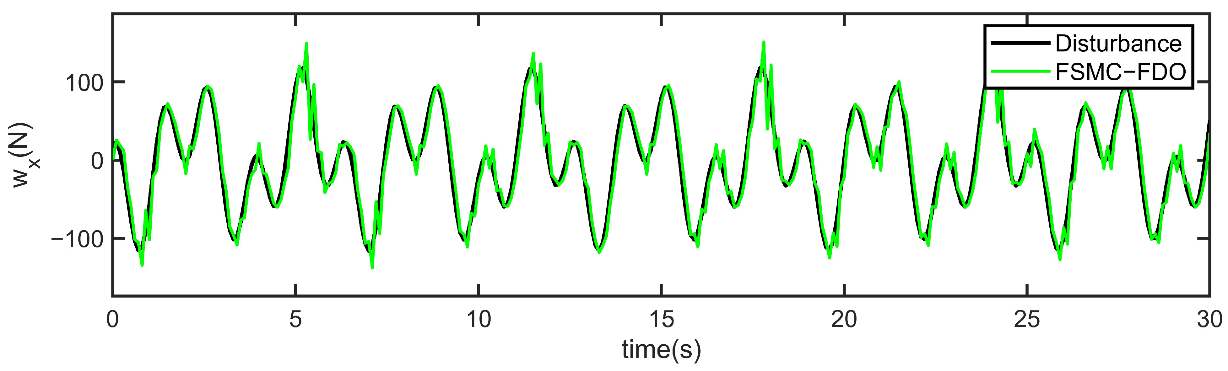
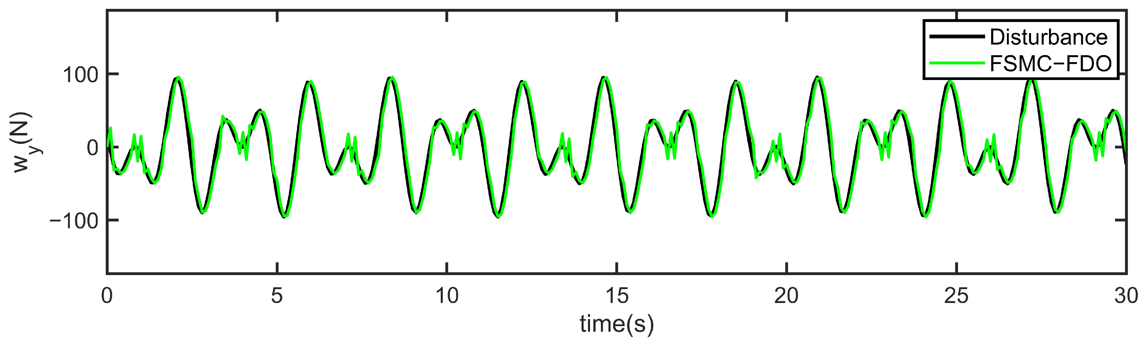
• A novel fixed-time disturbance observer is presented in order to compensate for ROVs model parameter errors and time-varying external disturbances. A Lyapunov analysis is used to demonstrate the stability of the system;
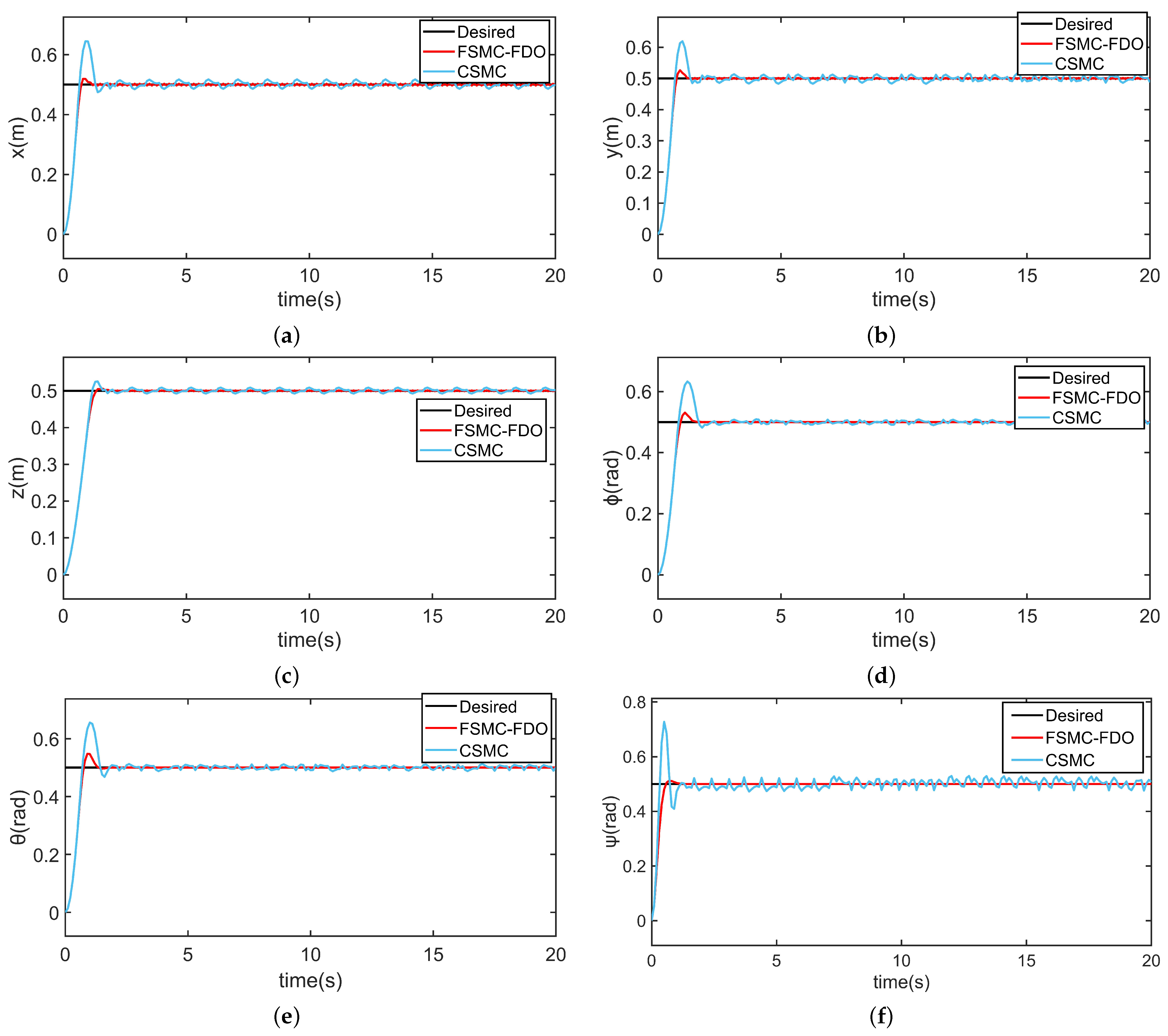
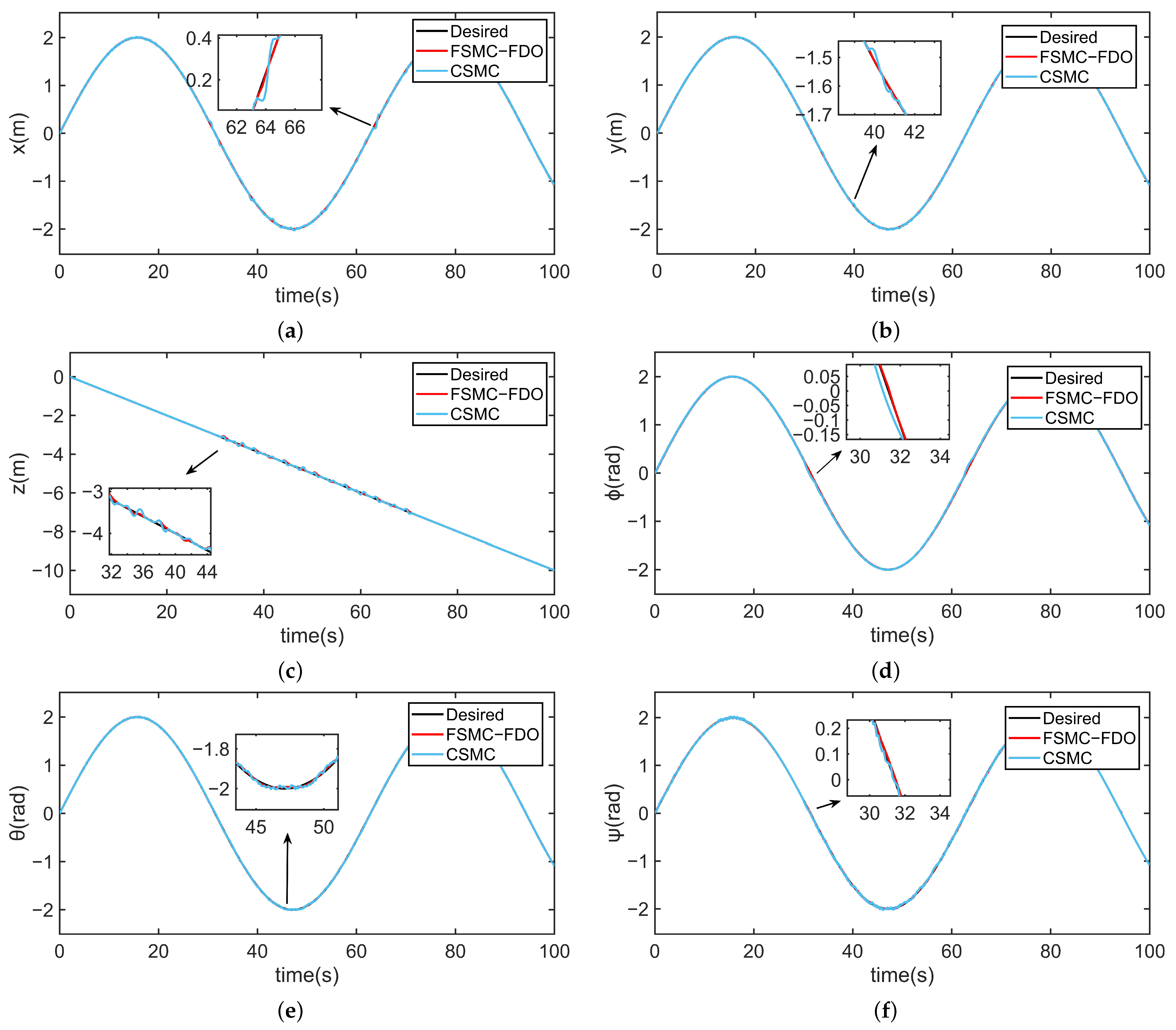
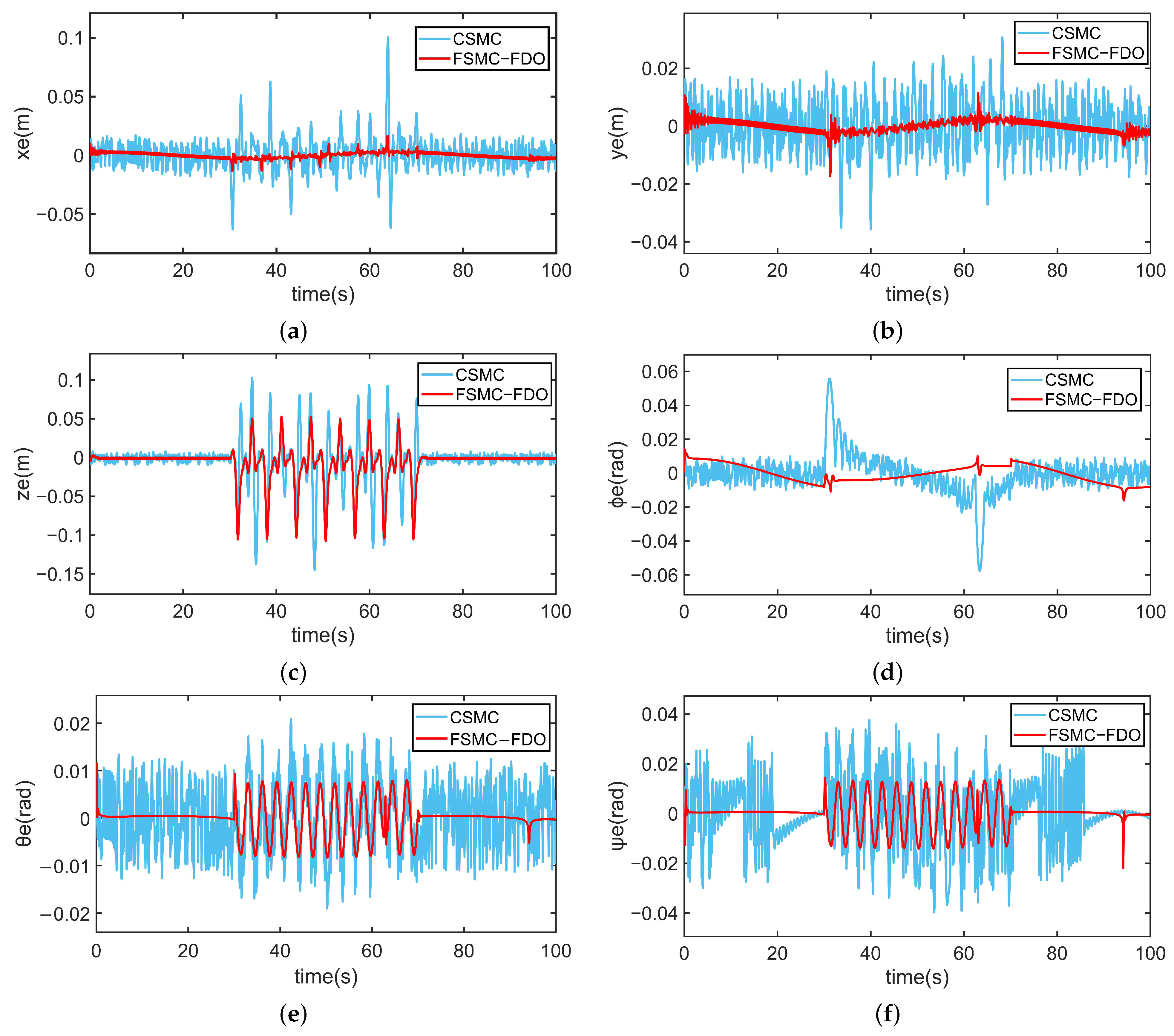
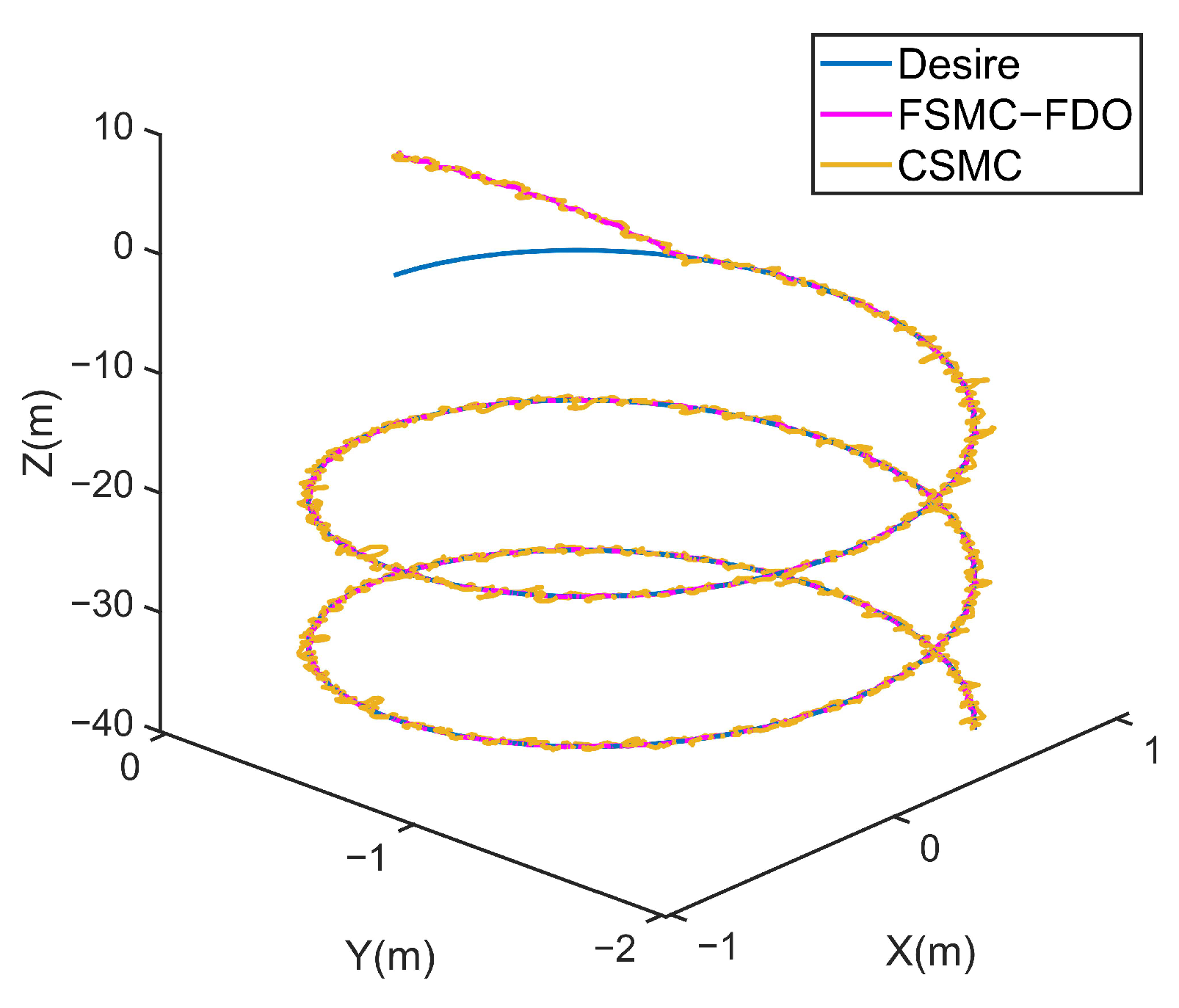
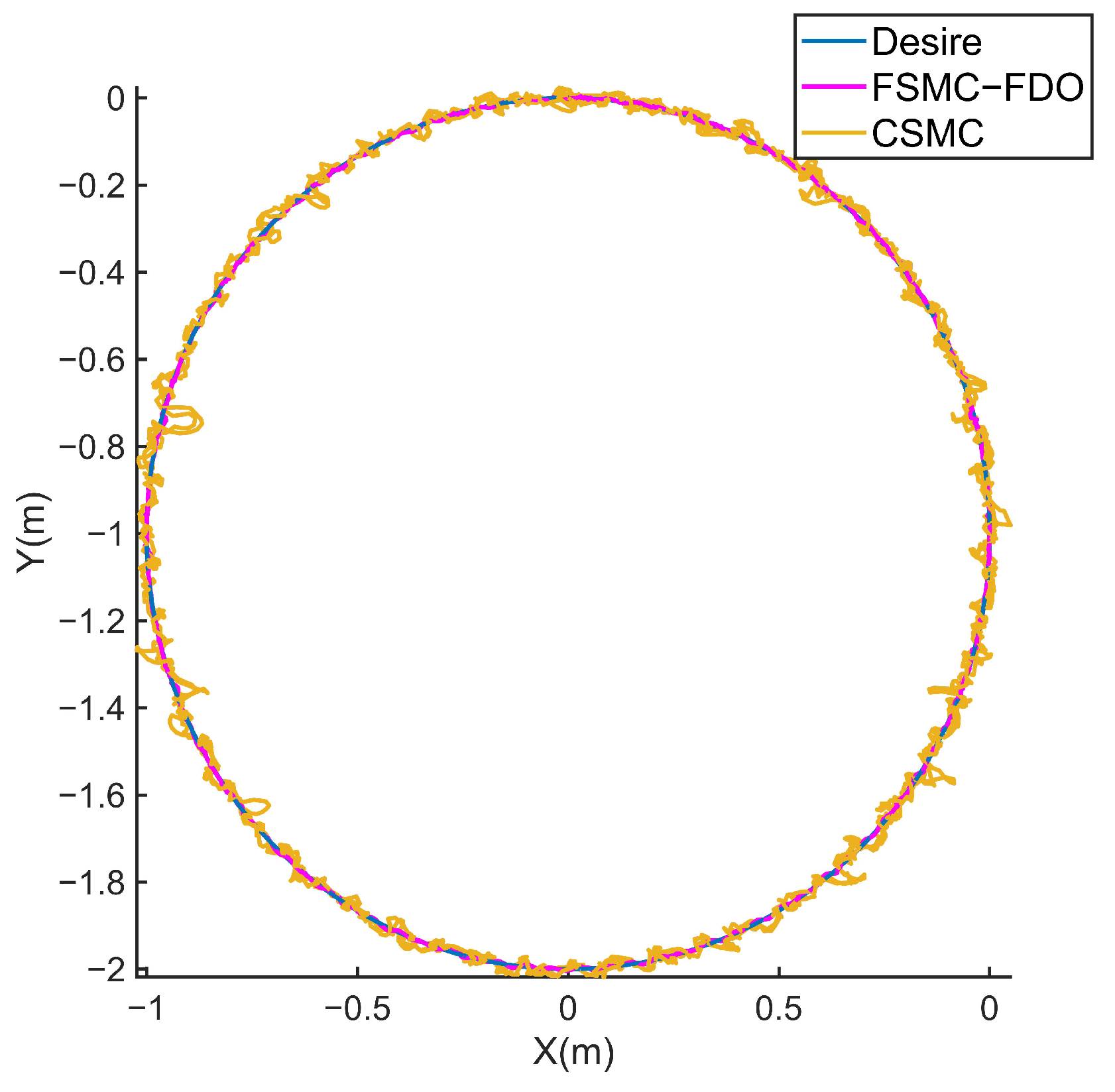
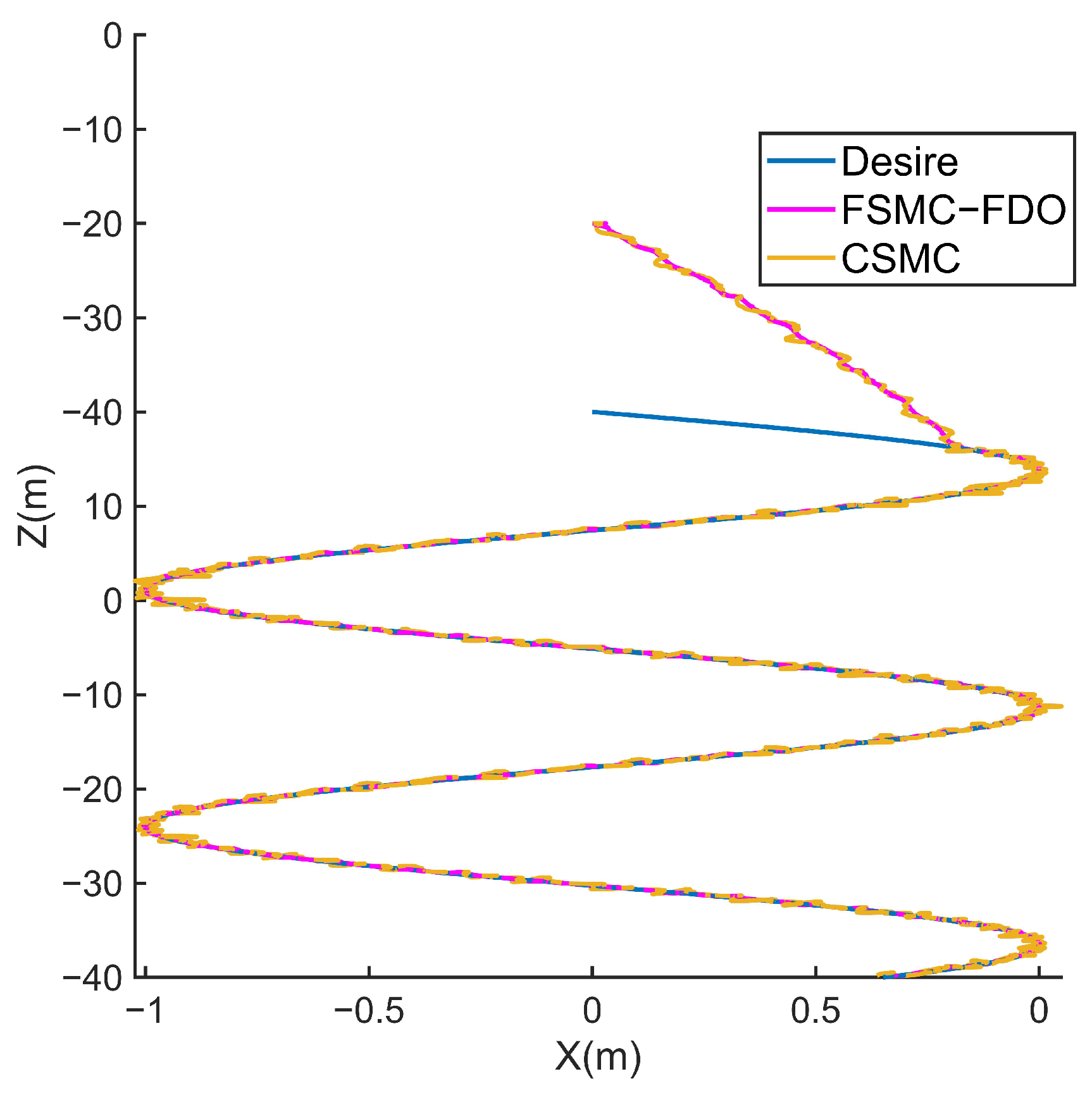
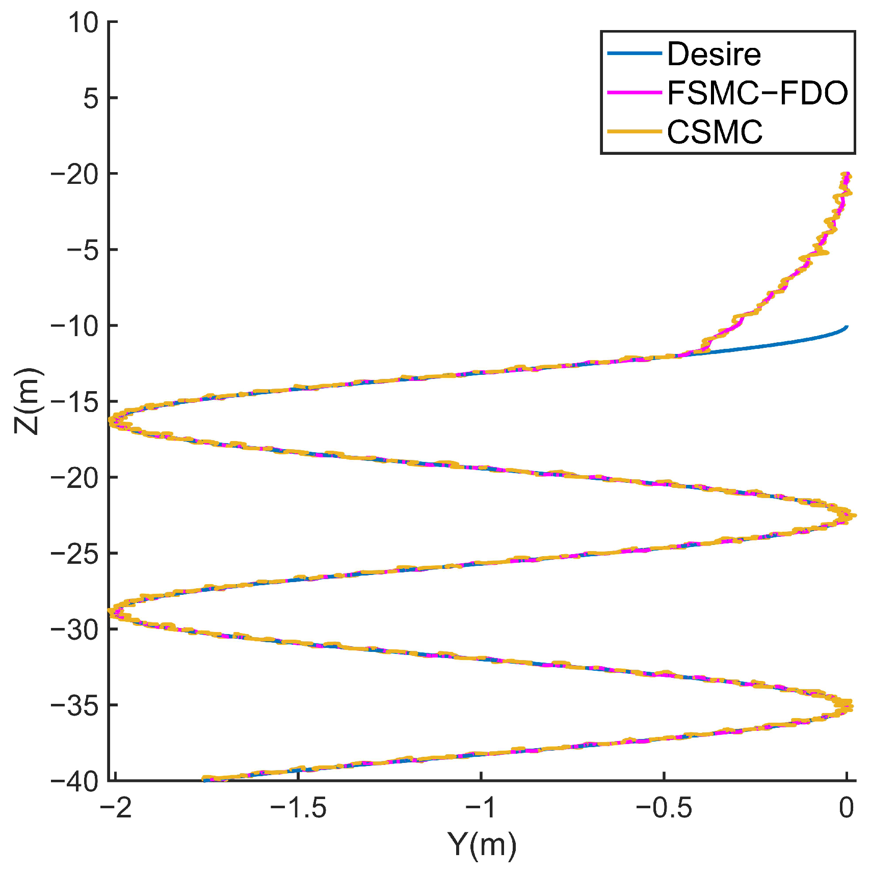
• To demonstrate the superior performance of the FSMC-FDO, a comparative study between the FSMC-FDO and the CSMC trajectory tracking is performed by simulation.

The remainder of the paper is organized as follows: the mathematical model of the underwater robot is described in Section 2. The control scheme is designed and stability analysis is presented in Section 3. Simulation results and comparative analysis are given in Section 4. Finally, conclusions are summarized in Section 5.

2. Preliminaries and Problem Statement

2.1. Preliminaries

Throughout this paper, for any vector $x\in \mathbb{R}$, $\left|x\right|$ represents the absolute value of x, $\left|\right|x\left|\right|$ is the Euclidean 2-norm and ${sig}^{\alpha }\left(x\right)=sgn\left(x\right){\left|x\right|}^{\alpha }$, where $sgn\left(x\right)$ is the function of the sign.

We define a fixed-time stable system to make the following lemma easier to understand.

Lemma 1

([22]). Consider the following nonlinear system:

$$\dot{x}\left(t\right)=f\left(x\right),f\left(0\right)=0,x\in {\mathbb{R}}^n$$

(1)

where $x={[x_1,x_2,\dots ,x_n]}^T$ and $f\left(x\right):{\mathbb{R}}^n\to {\mathbb{R}}^n$ is a nonlinear function.

Suppose there exists a positive define continuous Lyapunov function $V\left(x\right)$.

If

$$V\left(0\right)=0,\dot{V}\le -a{V}^{\alpha }\left(x\right)-b{V}^{\beta }\left(x\right)$$

(2)

then system (1) will be globally fixed-time stable and the settling time will satisfy the following:

$$T\le T_{max}=\frac{1}{a\left(1-\alpha \right)}+\frac{1}{b(1-\beta )}$$

(3)

where $a,b,\alpha ,\beta$ are positive parameters and $\alpha \in \left(0,1\right),\beta \in (1,+\infty )$.

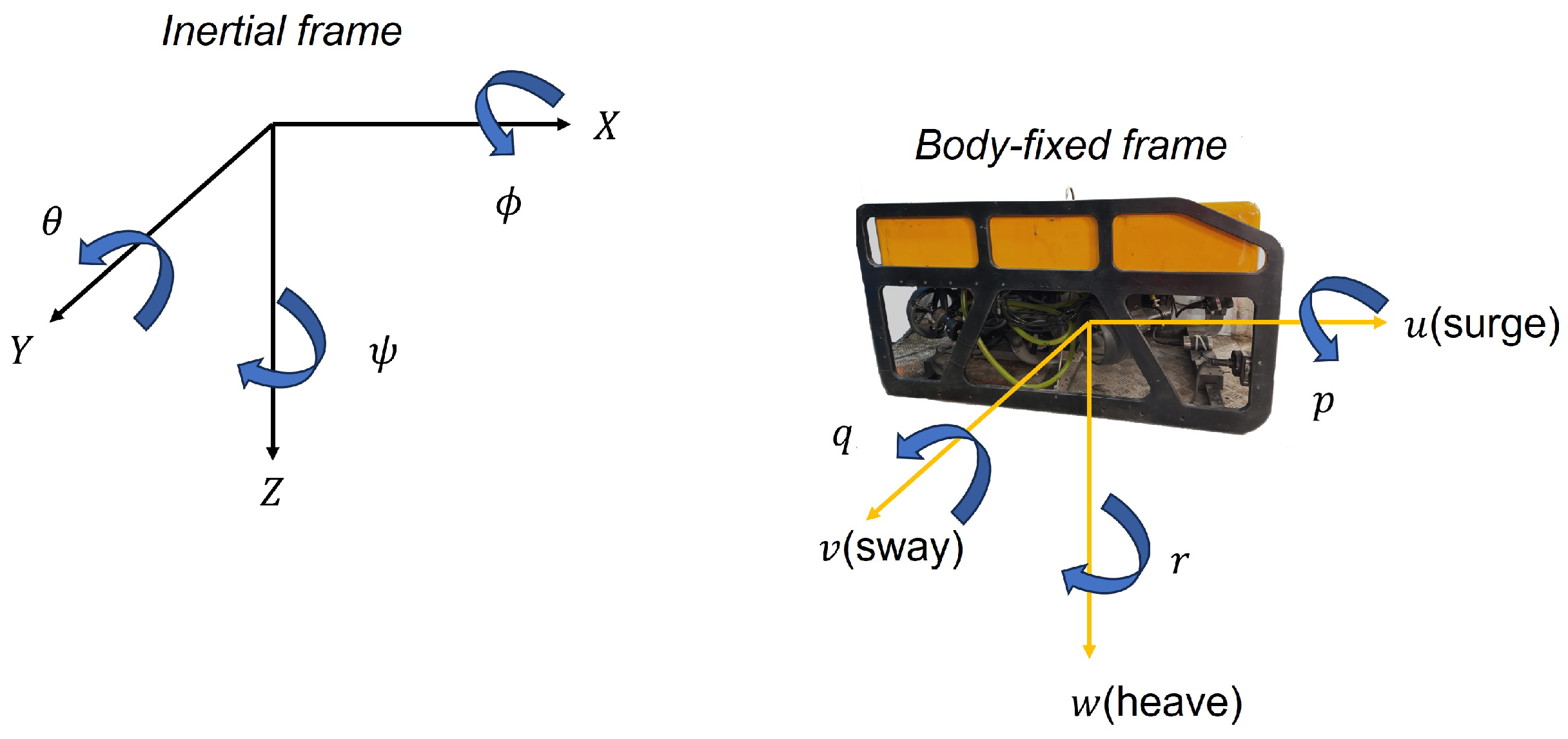
2.2. ROVs Kinematic and Dynamic Models

According to International Towing Tank Conference (ITTC) recommendations and the Society of Naval Architecture and Marine Engineers (SNAME) Terminology Bulletin System, as illustrated in Figure 1, the motions of ROVs are described by the following two co-ordinate frames: the center of mass of the ROVs is set as the origin of the inertial frame, and the positive direction of the inertial frame follows the positive direction of motion of the ROVs.

The following equation describes the kinematic model of an ROV:

$$\dot{\eta }=J\left(\eta \right)v$$

(4)

where $\eta ={\left[x,y,z,\varphi ,\theta ,\psi \right]}^T$ are the position and attitude vectors in the inertia frame, $[x,y,z]\in \mathbb{R}$ are the position coordinates, and $[\varphi ,\theta ,\psi ]\in \mathbb{R}$ are the attitude coordinates. The linear and angular velocity vectors in the body-fixed frame are represented by $v={\left[u,\upsilon ,w,p,q,r\right]}^T$, where $[u,\upsilon ,w]\in \mathbb{R}$ are the surge, sway, and heave velocities, and $[p,q,r]\in \mathbb{R}$ are the roll, pitch, and yaw velocities. $J\left(\eta \right){\in \mathbb{R}}^{6\times 6}$ is the transition matrix between the inertial and the body-fixed frame, which can be written as follows:

$$J\left(\eta \right)=\left[\begin{array}{cc}{J}_1\left(\eta \right)& 0_{3\times 3}\\ 0_{3\times 3}& J_2\left(\eta \right)\end{array}\right]$$

(5)

where $J_1\left(\eta \right)$ and $J_2\left(\eta \right)$ are denoted, respectively, as follows:

$$J_1\left(\eta \right)=\left[\begin{array}{ccc}cos\psi cos\theta & -sin\psi cos\varphi +cos\psi sin\theta sin\varphi & sin\psi sin\varphi +cos\psi sin\theta cos\varphi \\ sin\psi cos\theta & cos\psi cos\varphi +sin\psi sin\theta sin\varphi & -cos\psi sin\varphi +sin\psi sin\theta cos\varphi \\ -sin\theta & cos\theta sin\varphi & cos\theta cos\varphi \end{array}\right]$$

(6)

$$J_2\left(\eta \right)=\left[\begin{array}{ccc}1& sin\varphi tan\theta & cos\varphi tan\theta \\ 0& cos\varphi & -sin\varphi \\ 0& sin\varphi /cos\theta & cos\varphi /cos\theta \end{array}\right]$$

(7)

The ROVs’ dynamics model [15] can be expressed as follows:

$$M\dot{v}+C\left(v\right)\dot{v}+D\left(v\right)\dot{v}+G\left(\eta \right)=\tau +w$$

(8)

where $M{\in \mathbb{R}}^{6\times 6}$ is the inertia matrix including the added fluid inertia mass and rigid body inertia mass, $C\left(v\right){\in \mathbb{R}}^{6\times 6}$ is the Coriolis force and centripetal force matrix, $D\left(v\right){\in \mathbb{R}}^{6\times 6}$ represents the hydrodynamic damping matrix due to the surround fluid, also including the effects of added mass, $G\left(\eta \right){\in \mathbb{R}}^{6\times 1}$ is a restoring force and moment vector consisting of gravity and buoyancy, $\tau \left(\eta \right){\in \mathbb{R}}^{6\times 1}$ is the vector of the control forces and moments generated by the thruster acting on the ROVs and $w{\in \mathbb{R}}^{6\times 1}$ denotes the external disturbance vector.

The inertia matrix is $M=M_{RB}+M_A$, where $M_{RB}$ is the rigid body mass matrix and $M_A$ is the added mass matrix. The inertia matrix M can be expressed simply as follows:

$$M=\left[\begin{array}{cccccc}m-X_{\dot{u}}& 0& 0& 0& 0& 0\\ 0& m-Y_{\dot{v}}& 0& 0& 0& 0\\ 0& 0& m-Z_{\dot{w}}& 0& 0& 0\\ 0& 0& 0& I_x-K_{\dot{p}}& 0& 0\\ 0& 0& 0& 0& I_y-M_{\dot{q}}& 0\\ 0& 0& 0& 0& 0& I_z-N_{\dot{r}}\end{array}\right]$$

(9)

Considering the low cruising speed of the ROVs and that it can be approximated as a rigid-body symmetric structure, the Coriolis force and the centripetal force matrix $C\left(v\right)$ can be simplified to the following:

$$C\left(v\right)=\left[\begin{array}{cccccc}0& 0& 0& 0& \left(m-Z_{\dot{w}}\right)w& -\left(m+Y_{\dot{v}}\right)v\\ 0& 0& 0& -\left(m-Z_{\dot{w}}\right)w& 0& \left(m-X_{\dot{u}}\right)u\\ 0& 0& 0& \left(m-Y_{\dot{v}}\right)v& -\left(m-X_{\dot{u}}\right)u& 0\\ 0& \left(m-Z_{\dot{w}}\right)w& -\left(m-Y_{\dot{v}}\right)v& 0& I_{z}r& I_{y}q\\ -\left(m-Z_{\dot{w}}\right)w& 0& \left(m-X_{\dot{u}}\right)u& I_{z}r& 0& I_{x}p\\ \left(m-Y_{\dot{v}}\right)v& -\left(m-X_{\dot{u}}\right)u& 0& I_{y}q& I_{x}p& 0\end{array}\right]$$

(10)

Since hydrodynamic coupling is not significant at low ROV speeds, a higher order damping of the ROVs can be disregarded and only the first- and second-order damping needs to be considered. Thus, the hydrodynamic damping matrix $D\left(v\right)$ can be simplified to the following:

$$D\left(v\right)=-\left[\begin{array}{cccccc}{X}_u+X_{u\left|u\right|}\left|u\right|& 0& 0& 0& 0& 0\\ 0& Y_v+Y_{v\left|v\right|}\left|v\right|& 0& 0& 0& 0\\ 0& 0& Z_w+Z_{w\left|w\right|}\left|w\right|& 0& 0& 0\\ 0& 0& 0& K_p+K_{p\left|p\right|}\left|p\right|& 0& 0\\ 0& 0& 0& 0& M_q+M_{q\left|q\right|}\left|q\right|& 0\\ 0& 0& 0& 0& 0& N_r+N_{r\left|r\right|}\left|r\right|\end{array}\right]$$

(11)

Set the gravitational force W of the ROVs as equal to the buoyant force B, namely, $W=B$. Define the center of gravity coordinates as $[X_W,Y_W,Z_W]$ and the coordinates of the center of buoyancy as $[X_B,Y_B,Z_B]$, where $X_W=X_B=0$, $Y_W=Y_B=0$, $Z_B>Z_W=0$. Thus, $G\left(\eta \right)$ can be simplified to the following:

$$G\left(\eta \right)={[0,0,0,(Z_W-Z_B)Wcos\theta sin\varphi ,(Z_W-Z_B)Wsin\theta ,0]}^T$$

(12)

The ROVs model is very complex with a large number of unknown parameters; moreover, accurate hydrodynamic coefficients cannot be obtained. For this reason, and for the convenience of subsequent calculations, the actual kinetic model parameters M, C, D, G are treated as the sum of the estimated parameters $\overline{M}$, $\overline{C}$, $\overline{D}$, $\overline{G}$ and the uncertain parameters $M_{\Delta }$, $C_{\Delta }$, $D_{\Delta }$, $G_{\Delta }$ [23], whereby the actual dynamical model of ROVs can be transformed into the following:

$$\overline{M}\dot{v}+\overline{C}\left(v\right)v+\overline{D}\left(v\right)v+\overline{G}\left(\eta \right)={\tau }_{\eta }+w_{\eta }$$

(13)

where $\overline{M}=M-M_{\Delta }$, $\overline{C}=C-C_{\Delta }$, $\overline{D}=D-D_{\Delta }$, $\overline{G}=G-G_{\Delta }$, $w_{\eta }=w-M_{\Delta }\dot{v}-C_{\Delta }\left(v\right)v-D_{\Delta }\left(v\right)v-G_{\Delta }\left(\eta \right)$ and $w_{\eta }$ is the total unknown disturbance vector, containing the uncertain system dynamics parameters and environment disturbance effects.

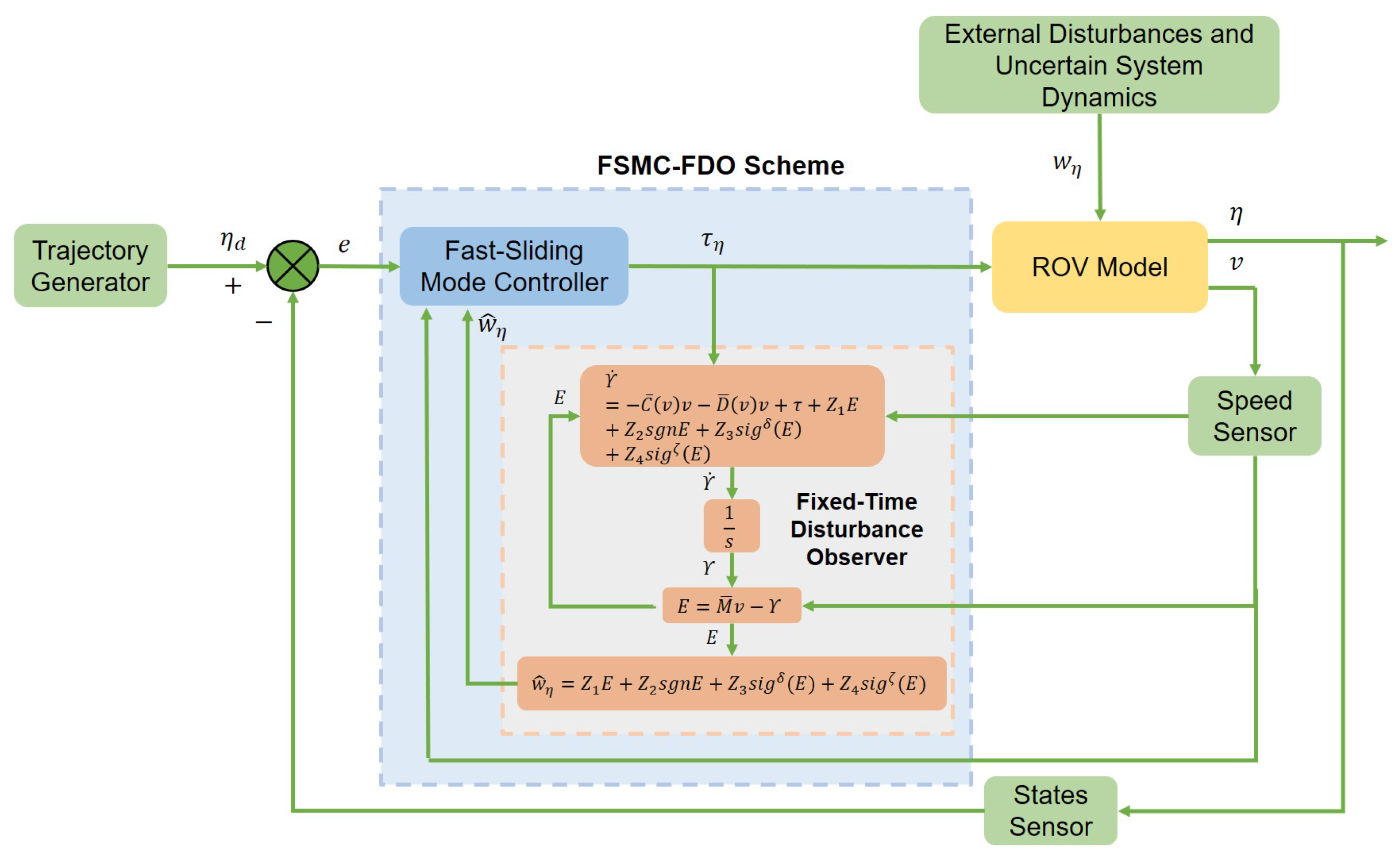
3. Control Scheme Design

In this section, a novel fast SMC scheme with a novel fixed-time disturbance observer is presented to improve the trajectory tracking ability of ROVs in time-varying environmental disturbances. First, an innovative reaching law is presented to resolve the contradiction between the system’s reaching time and the chatter amplitude in conventional SMC scheme. Then, a fixed-time disturbance observer is proposed to estimate and compensate for the external disturbances in an ROV’s working environment. Finally, the system stability analysis and verification is performed. The logic block diagram of the complete FSMC-FDO is illustrated in Figure 2.

3.1. Sliding Mode Control Scheme Design

A common form of an ROVs dynamics model is shown in Equation (13), and is used, for example, in [24,25]. In practice, by considering the complexity of subsequent computational modeling and simulations, the ROV dynamics model (13) can be rewritten in the form presented in [26] before designing an ROVs controller as follows:

$$\ddot{\eta }=\dot{J}\left(\eta \right)-J\left(\eta \right){\overline{M}}^{-1}(\overline{C}\left(v\right)v+\overline{D}\left(v\right)v+\overline{G}\left(\eta \right))+J\left(\eta \right){\overline{M}}^{-1}{w}_{\eta }$$

(14)

Conventional SMC is famous for its great robustness to ROV parameter inaccuracies and environmental disturbances. The desired $s{\in \mathbb{R}}^{6\times 1}$ is the sliding mode surface in sliding mode control theory, and e is denoted as the errors between the desired position and attitude ${\eta }_d$ and the actual position and attitude $\eta$, namely, the tracking errors $e={\eta }_d-\eta$. The traditional sliding mode surface usually is denoted as follows:

$$s=\Gamma e+\dot{e}$$

(15)

where $\Gamma {\in \mathbb{R}}^{6\times 6}$ is a positive definite constant diagonal gain matrix.

The standard SMC’s control law [27] consists of an equivalent control law ${\tau }_{eq}$ and a switching control law ${\tau }_{sw}$ as follows:

$$\tau ={\tau }_{eq}+{\tau }_{sw}$$

(16)

Theoretically, the equivalent control law is continuous, mainly reflecting the model’s information, and is capable of realizing the desired dynamic effect. When the state of the system reaches a specific sliding mode surface, then the equivalent control law can maintain this state on the sliding mode surface [28]. However, due to the existence of environmental disturbances and model uncertainty, switching control law is usually required to compensate the discrepancy between the estimated and actual dynamics. The control law of the switch is able to transfer the system state to the sliding mode surface.

Substituting (14) into (16) gives the following:

$$\begin{array}{cc}\dot{s}\hfill & =\Gamma \dot{e}+\ddot{e}=\Gamma \dot{e}+{\ddot{\eta }}_d-\ddot{\eta }\hfill \\ \hfill & =\Gamma \dot{e}+{\ddot{\eta }}_d-(\dot{J}\left(\eta \right)v-J\left(\eta \right){\overline{M}}^{-1}\left(\overline{C}\left(v\right)v+\overline{D}\left(v\right)v+\overline{G}\left(\eta \right)\right)\hfill \\ & +{J\left(\eta \right)\overline{M}}^{-1}\tau +J\left(\eta \right){\overline{M}}^{-1}{w}_{\eta })\hfill \end{array}$$

(17)

Assuming that $\dot{s}$ equals zero, the equivalent control law can be expressed as follows:

$$\begin{array}{cc}\hfill & {\tau }_{eq}=\overline{C}\left(v\right)v+\overline{D}\left(v\right)v+\overline{G}\left(\eta \right)+\overline{M}{J}^{-1}\left(\eta \right)\left(\Gamma \dot{e}+{\ddot{\eta }}_d-\dot{J}\left(\eta \right)v\right)-w_{\eta }\hfill \end{array}$$

(18)

3.2. Design and Analysis for the Reaching Law

In SMC, the switching control law ${\tau }_{sw}$ is determined by the reaching law. In this section, an innovative fast-reaching law (FRL) is presented to analyze the chatter characteristics. This law is able to deal with the conflict between the convergence time and the chatter amplitude in a conventional SMC scheme.

To clearly analyze the superiority of the FRL, it is required to introduce the CSMC ERL [18]. In SMC, the ERL can be described as follows:

$$\begin{array}{c}\dot{s}=-\epsilon s-ksgn\left(s\right)\hfill \end{array}$$

(19)

where $\epsilon$ and k are the gain matrices of the ERL, $\epsilon >0$, $k>0$, and $sgn(·)$ is the function of the sign. The sign function is a discontinuous function that causes discontinuity in the output of the switching control term, which, in turn, leads to chattering in the system.

The time for the state variable s to reach the sliding mode surface is defined as the response time $t_r$ of the ERL.

$$\begin{array}{c}{t}_r={\int }_{s_0}^{s_r}\frac{1}{-\epsilon s-ksgn\left(s\right)}ds\hfill \end{array}$$

(20)

where $s_0$ is the sliding mode surface value at the original instant ($t_0=0$), $s_r$ is the state variable at the first time the system reaches the sliding mode surface, and $s_r=0$.

Because the value of $s_0$ is uncertain, (20) needs to be examined for the following three cases: $s_0>0$, $s_0=0$, $s_0<0$.

Case 1: If $s_0>0$, according to SMC theory, $s>0$ in the time interval $[t_0,t_r]$. At this time, the following equation can be obtained from (20):

$$\begin{array}{c}{t}_{r+}=\frac{1}{\epsilon }ln(\frac{\epsilon }{k}{s}_0+1)\hfill \end{array}$$

(21)

Case 2: If $s_0=0$, according to SMC theory, $s=0$ in the time interval $[t_0,t_r]$. At this point, the state variable of the system is on the sliding mode surface; therefore,

$$\begin{array}{c}{t}_r=0\hfill \end{array}$$

(22)

Case 3: If $s_0<0$, according to SMC theory, $s=0$ in the time interval $[t_0,t_r]$. At this time, the following equation can be obtained from (20):

$$\begin{array}{c}{t}_{r-}=\frac{1}{\epsilon }ln(-\frac{\epsilon }{k}{s}_0+1)\hfill \end{array}$$

(23)

In summary, the response time of the ERL can be expressed as follows:

$$\begin{array}{c}{t}_r=\frac{1}{\epsilon }ln(\frac{\epsilon }{k}{|s}_0|+1)\hfill \end{array}$$

(24)

To analyze the chattering by discretizing this expression, in digital control, (19) can be rewritten as follows:

$$\begin{array}{c}\frac{s(N+1)-s\left(N\right)}{T_s}=-\epsilon s\left(N\right)-ksgn\left(s\left(N\right)\right)\hfill \end{array}$$

(25)

where $T_s$ is the sample period.

When the state variable of the system reaches the sliding mode surface in limited time. Following the SMC theory, the system state variable will oscillate around the sliding mode surface, namely, $s\left(N\right)\to 0^{+}$ or $s\left(N\right)\to 0^{-}$. Moreover, $-\epsilon s\left(N\right)$ in (25) can be neglected when the state variable of the system reaches the neighborhood of the sliding surface.

Thus, when $s\left(N\right)\to 0^{+}$, the following is obtained:

$$\begin{array}{c}s\left(N+1\right)=-k{T}_s\hfill \end{array}$$

(26)

When $s\left(N\right)\to 0^{-}$, the following is obtained:

$$\begin{array}{c}s\left(N+1\right)=k{T}_s\hfill \end{array}$$

(27)

Therefore, the chatter amplitude of the ERL is as follows:

$$\begin{array}{c}{\Delta }_r=2k{T}_s\hfill \end{array}$$

(28)

By analyzing (24) and (28), it can be observed that increasing $\epsilon$ will decrease the response time $t_r$ and vice versa when the system state variable of the system is distant away from the sliding mode surface s. However, changing the values of $\epsilon$ when the state variable of the system is approaching the sliding mode surface s has a negligible effect on the response time $t_r$; moreover, increases in the gain k will decrease the response time $t_r$ but will increase the chatter amplitude ${\Delta }_r$, and decreases in the gain k will decrease the chatter amplitude ${\Delta }_r$ but will increase the response time $t_r$. Therefore, in conventional sliding mode control using the ERL, an irreconcilable contradiction exists between the response time of the system and the magnitude of the chatter.

Based on the idea of the ERL, a novel FRL is proposed in this paper as follows:

$$\begin{array}{c}\dot{s}=-\frac{\mu \left|s_0\right|+\left|s\right|}{\left(\alpha +\beta \right)\mu \left|s_0\right|+\alpha \left|s\right|}·ksgn\left(s\right)-ktanh\left(s\right)\hfill \end{array}$$

(29)

where $\alpha$, $\beta$, $\mu$, and k are the gain matrices of the FRL, $0<\alpha <1$, $\beta >1$, $\mu >0$, and $k>0$. $tanh(·)$ is the hyperbolic tangent function. $s_0$ is the original position of the state variable, i.e., the state variable at the time $t_0=0$.

The FRL, like the ERL principle, increases the convergence speed of the system state when it is farther away from the sliding surface and decreases the convergence speed of the system when it is closer to the sliding surface. The advantage of (29) is that the convergence speed decreases faster than (19) when the system state is close to the sliding surface, which reduces the effect of system inertia when the system state passes through the sliding surface.

Assuming the time at which the state variable of the system first reaches the sliding mode surface is $t_c$, its position at this time is $s_c$, and according to the SMC theory, it can be shown at this time that $s_c=0$.

Thus, the reach time $t_c$ can be obtained by integrating (29) as follows:

$$\begin{array}{c}{t}_c=-\frac{1}{k}{\int }_{s_0}^{s_c}\left[\frac{\left(\alpha +\beta \right)\mu \left|s_0\right|+\alpha \left|s\right|}{\mu \left|s_0\right|+\left|s\right|}·\frac{1}{sgn\left(s\right)}-\frac{1}{tanh\left(s\right)}\right]\hfill \end{array}$$

(30)

As with the ERL, the value of $s_0$ is unknown, and therefore must be considered for the following three cases: $s_0>0$, $s_0=0$, and $s_0<0$.

Case 1: If $s_0>0$, according to SMC theory, $s>0$ in the time interval $[t_0,t_c]$. At this point, we can obtain the following equation from (30):

$$\begin{array}{c}{t}_{c+}=\frac{s_0}{k}[\alpha +\beta ·\mu ·ln(1+{\mu }^{-1})]-ln(1-s_0^2)\hfill \end{array}$$

(31)

Case 2: If $s_0=0$, according to SMC theory, $s=0$ in the time interval $[t_0,t_c]$. At this point, the state variable of the system is located on the sliding mode surface; therefore,

$$\begin{array}{c}{t}_c=0\hfill \end{array}$$

(32)

Case 3: If $s_0<0$, according to SMC theory, $s<0$ in the time interval $[t_0,t_c]$. At this point, we can obtain the following equation from (30):

$$\begin{array}{c}{t}_{c-}=-\frac{s_0}{k}[\alpha +\beta ·\mu ·ln(1+{\mu }^{-1})]-ln(1-s_0^2)\hfill \end{array}$$

(33)

To summarize, the FRL response time can be expressed as follows:

$$\begin{array}{c}{t}_c=\frac{{|s}_0|}{k}[\alpha +\beta ·\mu ·ln(1+{\mu }^{-1})]-ln(1-s_0^2)\hfill \end{array}$$

(34)

Consideration of sliding motion features as the system state variable moves onto the sliding mode surface, (29) can be simplified to (35) as follows:

$$\begin{array}{c}\dot{s}=-\frac{k}{\left(\alpha +\beta \right)}·sgn\left(s\right)\hfill \end{array}$$

(35)

When the state of the system is far from the sliding surface, it is converged as shown in (29), and when the system is close to the sliding surface, the value of s is so small that it can be neglected. Thus, (35) can be regarded as a special stage of (29). Compared to (35), (29) is more concise and can reduce the complexity of the later equation for chattering amplitude. This helps in the subsequent analysis of the effect of each parameter on the chattering amplitude.

The same processing used for the ERL is used to obtain the chatter amplitude ${\Delta }_c$ of the FRL using the following discretization method:

$$\begin{array}{c}{\Delta }_c=\frac{2k}{\alpha +\beta }{T}_s\hfill \end{array}$$

(36)

where $T_s$ is the sample period.

By analyzing (34) and (36), it can be found that the value of $\mu ·ln(1+{\mu }^{-1})$ increases with $\mu$ when $\mu \in (0,\infty )$. By increasing the value of $\alpha$, the response time $t_c$ will increase, but the chatter amplitude ${\Delta }_c$ will consequently decrease. By decreasing the value of $\alpha$, the response time $t_c$ will decrease, but the chatter amplitude ${\Delta }_c$ will subsequently increase. When increasing $\alpha$, the response time $t_c$ cannot be reduced by other means, but when decreasing the value of $\alpha$, the chatter amplitude ${\Delta }_c$ can be reduced by increasing the value of $\beta$; therefore, $\beta$ needs to be set to a large value, while increasing the value of $\beta$, the response time $t_c$ will increase, but the chatter amplitude ${\Delta }_c$ will decrease; in which case, the response time $t_c$ can be reduced by setting a sufficiently small $\mu$. Therefore, the contradiction in the ERL can be resolved by designing the values of the parameters $\alpha$, $\beta$, and $\mu$ so that the response time is small in addition to the chatter amplitude. Moreover, the previous analysis shows in which direction the parameters should be adjustment, reducing the difficulty of parameter adjustment.

Considering the above, the SMC switch control law ${\tau }_{sw}$ can be expressed as follows:

$$\begin{array}{c}{\tau }_{sw}=\overline{M}{J}^{-1}\left(\eta \right)\left[\frac{\mu \left|s_0\right|+\left|s\right|}{\left(\alpha +\beta \right)\mu \left|s_0\right|+\alpha \left|s\right|}·ksgn\left(s\right)+ktanh\left(s\right)\right]\hfill \end{array}$$

(37)

Thus, the SMC control law can be obtained from (18) and (37) as follows:

$$\begin{array}{cc}\tau \hfill & =\overline{C}\left(v\right)v+\overline{D}\left(v\right)v+\overline{G}\left(\eta \right)+\overline{M}{J}^{-1}\left(\eta \right)(\Gamma \dot{e}+{\ddot{\eta }}_d-\dot{J}\left(\eta \right)v\hfill \\ \hfill & +\frac{\mu \left|s_0\right|+\left|s\right|}{\left(\alpha +\beta \right)\mu \left|s_0\right|+\alpha \left|s\right|}·ksgn\left(s\right)+ktanh\left(s\right))-w_{\eta }\left(t\right)\hfill \end{array}$$

(38)

3.3. Stability Analysis

Lyapunov is a virtual energy function used to verify the stability of a system. Suitable Lyapunov functions can provide influence on the values of the parameters in the control law to enhance the stability performance of the system [29,30]. The selection of the Lyapunov function is generally related to the error, and the tracking error and the unknown parameter error were selected as the parameters of the Lyapunov function in [30].

In the sliding mode control part of this paper, only the tracking error needs to be considered, so the following quadratic Lyapunov function is chosen to verify the stability of the system:

$$\begin{array}{c}{V}_1=\frac{1}{2}{s}^{T}s\hfill \end{array}$$

(39)

Combining (17), (29), (38), and (39), the time derivative ${\dot{V}}_1$ of $V_1$ can be written as follows:

$$\begin{array}{cc}{\dot{V}}_1\hfill & =s^T\left(\Gamma \dot{e}+{\ddot{\eta }}_d-\left(\dot{J}\left(\eta \right)v-J\left(\eta \right){\overline{M}}^{-1}\left(\overline{C}\left(v\right)v+\overline{D}\left(v\right)v+\overline{G}\left(\eta \right)\right)+{J\left(\eta \right)\overline{M}}^{-1}\tau +J\left(\eta \right){\overline{M}}^{-1}{w}_{\eta }\right)\right)\hfill \\ \hfill & =s^T\left(-\frac{\mu \left|s_0\right|+\left|s\right|}{\left(\alpha +\beta \right)\mu \left|s_0\right|+\alpha \left|s\right|}·ksgn\left(s\right)-ktanh\left(s\right)\right)\hfill \\ \hfill & \le s^T\left(-\frac{\mu \left|s_0\right|+\left|s\right|}{\left(\alpha +\beta \right)\mu \left|s_0\right|+\alpha \left|s\right|}·ksgn\left(s\right)\right)\hfill \end{array}$$

(40)

The value ranges of the $\alpha$, $\beta$, $\mu$, and k parameters have been defined previously. Thus, in (40), it is obvious that $-\frac{\mu \left|s_0\right|+\left|s\right|}{\left(\alpha +\beta \right)\mu \left|s_0\right|+\alpha \left|s\right|}<0$ and $s^T·ksgn\left(s\right)\ge 0$, which leads to ${\dot{V}}_1\le 0$. Thus, the system can be shown to be globally asymptotically stable.

3.4. Fixed-Time Disturbance Observer

In practice, ROVs are affected by various complex environmental forces and modeling errors. After this, the dynamics cannot be restored to their actual state, so it is necessary to a design disturbance observer for online estimation of and compensation for uncertain disturbances.

Assumption 1.

External disturbance changes are relatively slow.

Assumption 2.

The aggregate uncertainty $w_{\eta }$ of the system dynamics is bounded, namely, there exists a nonzero constant ρ satisfying $\left|\right|w_{\eta }\left|\right|\le \rho \le \infty$.

Assumption 3.

Each element in the parameter matrix $Z_2$ is greater than ρ.

We first define the error variable E as follows:

$$\begin{array}{c}E=\overline{M}v-{\rm Y}\hfill \end{array}$$

(41)

where v is the velocity variable of the ROVs, ${\rm Y}$ is the dynamical auxiliary variable of the introduced disturbance observer with the same dimension as the velocity and ${\rm Y}$ is as follows:

$$\begin{array}{c}\dot{{\rm Y}}=-\overline{C}\left(v\right)v-\overline{D}\left(v\right)v+{\tau }_{\eta }+Z_{1}E+Z_{2}sgnE+Z_3{sig}^{\delta }\left(E\right)+Z_4{sig}^{\zeta }\left(E\right)\hfill \end{array}$$

(42)

where $Z_i\in {\mathbb{R}}^{6\times 1}(i=1,2,3,4)$ are positive definite diagonal matrices and ${\lambda }_{min}\left(Z_2\right)\ge \rho$. That is, every element in the diagonal matrix $Z_2$ is greater than or equal to $\rho$. $\delta$ and $\zeta$ are positive constants, with $0<\delta <1$, $\zeta >1$.

The derivative of E is as follows:

$$\begin{array}{cc}\dot{E}\hfill & =\overline{M}\dot{v}-\dot{{\rm Y}}\hfill \\ \hfill & =-\overline{C}\left(v\right)v-\overline{D}\left(v\right)v+{\tau }_{\eta }+w_{\eta }-[-\overline{C}\left(v\right)v-\overline{D}\left(v\right)v+{\tau }_{\eta }\hfill \\ \hfill & +Z_{1}E+Z_{2}sgnE+Z_3{sig}^{\delta }\left(E\right)+Z_4{sig}^{\zeta }\left(E\right)]\hfill \\ \hfill & =w_{\eta }-Z_{1}E-Z_{2}sgnE-Z_3{sig}^{\delta }\left(E\right)-Z_4{sig}^{\zeta }\left(E\right)\hfill \end{array}$$

(43)

Designing a fixed-time disturbance observer ${\widehat{w}}_{\eta }$ enables (43) to converge as follows:

$$\begin{array}{c}{\widehat{w}}_{\eta }=Z_{1}E+Z_{2}sgnE+Z_3{sig}^{\delta }\left(E\right)+Z_4{sig}^{\zeta }\left(E\right)\hfill \end{array}$$

(44)

To evaluate the performance of the fixed-time disturbance observer, we define the estimation error variable ${\tilde{w}}_{\eta }$ as follows:

$$\begin{array}{c}{\tilde{w}}_{\eta }=w_{\eta }-{\widehat{w}}_{\eta }=w_{\eta }-Z_{1}E-Z_{2}sgnE-Z_3{sig}^{\delta }\left(E\right)-Z_4{sig}^{\zeta }\left(E\right)\hfill \end{array}$$

(45)

Under the action of (44), this estimation error will gradually converge to zero. The proof is as follows:

From (45), if E converges, then its derivative $\dot{E}$ also converges, and thus ${\tilde{w}}_{\eta }$ can also converge.

Define the Lyapunov function $V_E$ as follows:

$$\begin{array}{c}{V}_E=\frac{1}{2}{E}^{T}E\hfill \end{array}$$

(46)

$$\begin{array}{cc}{\dot{V}}_E\hfill & =E^T\dot{E}\hfill \\ \hfill & =E^T\left[w_{\eta }-Z_{1}E-Z_{2}sgnE-Z_3{sig}^{\delta }\left(E\right)-Z_4{sig}^{\zeta }\left(E\right)\right]\hfill \\ \hfill & \le \rho \left|\left|E\right|\right|-Z_1{\left|\left|E\right|\right|}^2-Z_2\left|\left|E\right|\right|-E^T\left(Z_3{E}^{\delta }+Z_4{E}^{\zeta }\right)\hfill \\ \hfill & \le -Z_3{\left(E^{T}E\right)}^{\frac{\delta +1}{2}}-Z_4{\left(E^{T}E\right)}^{\frac{\zeta +1}{2}}\hfill \\ \hfill & =-2^{\frac{\delta +1}{2}}{\lambda }_{min}\left(Z_3\right){\left(\frac{1}{2}{E}^{T}E\right)}^{\frac{\delta +1}{2}}-2^{\frac{\zeta +1}{2}}{\lambda }_{min}\left(Z_4\right){\left(\frac{1}{2}{E}^{T}E\right)}^{\frac{\zeta +1}{2}}\hfill \\ \hfill & =-2^{\frac{\delta +1}{2}}{\lambda }_{min}\left(Z_3\right)V_E^{\frac{\delta +1}{2}}-2^{\frac{\zeta +1}{2}}{\lambda }_{min}\left(Z_4\right)V_E^{\frac{\zeta +1}{2}}\hfill \end{array}$$

(47)

where the function ${\lambda }_{min}(•)$ is the minimum eigenvalue of the matrix.

By Lemma 1 it can be shown that E is fixed-time stable. The upper bound of the convergence time of the system is given by the following:

$$\begin{array}{c}{T}_0\le T_{max}=\frac{2^{\frac{1-\delta }{2}}}{{\lambda }_{min}\left(Z_3\right)\left(1-\delta \right)}+\frac{2^{\frac{1-\zeta }{2}}}{{\lambda }_{min}\left(Z_4\right)(\zeta -1)}\hfill \end{array}$$

(48)

This shows that $E=0$ when the system time $t\ge T_0$, which leads to the conclusion that ${\widehat{w}}_{\eta }=0$ when $t\ge T_0$.

4. Simulation Study and Results Discussion

In this section, the effectiveness and superiority of the designed controller is verified by a numerical simulation using MATLAB/Simulink R2021b software. The simulation results are given for the FSMC-FDO and CSMC based on the ERL [31]. The ROVs model parameters used in the simulation are provided in

Table 1. ROVs system parameters.

Parameter	Value	Parameter	Value
$X_u$	− 36.27 N/s	$N_{\dot{r}}$	−6.23 kg
$Y_v$	−43.72 N/s	$X_{u\left|u\right|}$	−9.44 ${\mathrm{N}}^2/{\mathrm{m}}^2$
$Z_w$	−105.29 N/s	$Y_{v\left|v\right|}$	−13.53 ${\mathrm{N}}^2/{\mathrm{m}}^2$
$K_p$	−7.86 N/s	$Z_{w\left|w\right|}$	−35.62 ${\mathrm{N}}^2/{\mathrm{m}}^2$
$M_q$	−8.16 N/s	$K_{p\left|p\right|}$	−10.65 ${\mathrm{N}}^2/{\mathrm{m}}^2$
$N_r$	−10.21 N/s	$M_{q\left|q\right|}$	−9.23 ${\mathrm{N}}^2/{\mathrm{m}}^2$
$X_{\dot{u}}$	−17.25 kg	$N_{r\left|r\right|}$	−102.32 ${\mathrm{N}}^2/{\mathrm{m}}^2$
$Y_{\dot{v}}$	−20.22 kg	$I_x$	10.13 ${\mathrm{Nms}}^2$
$Z_{\dot{w}}$	−22.73 kg	$I_y$	16.48 ${\mathrm{Nms}}^2$
$K_{\dot{p}}$	−2.65 kg	$I_z$	17.52 ${\mathrm{Nms}}^2$
$M_{\dot{q}}$	−1.23 kg	m	23.5 kg

.

To further compare the performance of the different schemes, the following three measurements are introduced: the first, the overshoot, also called the maximum deviation, is a measure of the control system’s dynamic performance in a step response. The average of the absolute deviations of all individual values from the arithmetic mean is the mean absolute error (MAE). The mean absolute error solves the problem of errors canceling each other out, and thus accurately reflects the actual error magnitude. A measure of the average deviation from the true value is the root mean square error (RMSE). The three measures are defined in the following:

$$\begin{array}{c}overshoot=({\eta }_{max}-\eta \left(\infty \right))\times 100\%\hfill \end{array}$$

(49)

$$\begin{array}{c}MAE=\frac{1}{n}\sum _{i=1}^n|{\eta }_i-{\eta }_{di}|\hfill \end{array}$$

(50)

$$\begin{array}{c}RMSE=\sqrt{\frac{1}{n}\sum _{i=1}^n{({\eta }_i-{\eta }_{di})}^2}\hfill \end{array}$$

(51)

The fast sliding control scheme parameters were selected as follows:

$\alpha =diag[0.04,0.01,0.05,0.01,0.01,0.01]$, $\beta =diag[4\times {10}^5,4\times {10}^5,5\times {10}^5,4\times {10}^5,5\times {10}^5,5\times {10}^5]$, $\mu =diag[0.001,0.001,0.001,0.001,0.001,0.001]$, $k=diag[2,2,1,4,1,1]$, $\Gamma =diag[26,5,1,15,27,16]$.

The fixed-time disturbance observer parameters were set as follows:

$Z_1=diag[4,3,5]$, $Z_2=diag[0.1,0.1,0.1]$, $Z_3=diag[10,10,10]$, $Z_4=diag[2,1,2]$, $\delta =0.1$, $\zeta =2$.

Three cases of simulation will be considered here.

Case 1: For the verification of the superiority of the proposed FSMC-FDO scheme, a comparison with the CSMC scheme is performed. Step-response reference trajectory tracking of six degrees of freedom (DOF) in a no-external-disturbance scenario was performed for the FSMC-FDO scheme and the CSMC scheme. The original state of the ROVs is set to the following:

$x\left(0\right)=y\left(0\right)=z\left(0\right)=0\mathrm{m}$, $\varphi \left(0\right)=\theta \left(0\right)=\psi \left(0\right)=0\mathrm{rad}$, $u\left(0\right)=v\left(0\right)=w\left(0\right)=0\mathrm{m}/\mathrm{s}$, $p\left(0\right)=q\left(0\right)=r\left(0\right)=0\mathrm{r}\mathrm{a}\mathrm{d}/\mathrm{s}$.

The simulation time is 20 s and the final position and attitude of the ROVs are as follows:

$x\left(0\right)=y\left(0\right)=z\left(0\right)=0.5\mathrm{m}$, $\varphi \left(0\right)=\theta \left(0\right)=\psi \left(0\right)=0.5\mathrm{rad}$.

The response curves of the two control schemes at different DOF are shown in Figure 3.

Figure 3 shows the step response capabilities of the two control schemes for position and attitude in each of the six DOF. The FSMC-FDO scheme has faster convergence and less chatter than the CSMC scheme, as shown in the figure.

Table 2. Comparison of the overshoot performance of different control schemes in Case 1.

Parameters	Values	Parameters	Values
x	14.81%	x	23.91%
y	11.08%	y	27.01%
z	2.75%	z	4.58%
$\varphi$	11.19%	$\varphi$	26.22%
$\theta$	7.72%	$\theta$	30.88%
$\psi$	2.40%	$\psi$	40.03%

summarizes the overshoot degree for the two schemes under the step response, and it is clearly seen that the overshoot of the FSMC-FDO scheme is lower than that of the CSMC scheme by between $1.83\%$ and $40.63\%$. This phenomenon highlights the significant superiority of the FSMC-FDO in terms of fixed-time convergence and the precision of convergence.

Case 2: To evaluate the robustness of the presented FSMC-FDO scheme, trajectory tracking simulations were performed with time-varying external disturbances using both control schemes. The initial state of the ROVs was the same as in Case 1, and the desired trajectory of the motion of the six DOF was as follows:

$$\begin{array}{c}\left\{\begin{array}{c}x=2sin\left(0.1t\right)\mathrm{m}\hfill \\ y=2sin\left(0.1t\right)\mathrm{m}\hfill \\ z=-0.1t\mathrm{m}\hfill \\ \varphi =2sin\left(0.1t\right)\mathrm{rad}\hfill \\ \theta =2sin\left(0.1t\right)\mathrm{rad}\hfill \\ \psi =2sin\left(0.1t\right)\mathrm{rad}\hfill \end{array}\right.\hfill \end{array}$$

(52)

In this case, the simulation time was set to 100 s and external disturbances between 30 s and 70 s were added as follows:

$$\begin{array}{l}\left\{\begin{array}{c}{w}_x=60\left[cos\left(5t-120\right)+cos\left(2t+90\right)\right]\mathrm{N}\hfill \\ w_y=50\left[cos\left(5t+90\right)+sin\left(3t+90\right)\right]\mathrm{N}\hfill \\ w_z=60\left[cos\left(5t+120\right)+sin\left(3t+90\right)\right]\mathrm{N}\hfill \\ w_{\varphi }=40cos\left(2t\right)\mathrm{N}·\mathrm{m}\hfill \\ w_{\theta }=50cos\left(2t\right)\mathrm{N}·\mathrm{m}\hfill \\ w_{\psi }=50cos\left(2t\right)\mathrm{N}·\mathrm{m}\hfill \end{array}\right.\hfill \end{array}$$

(53)

Trajectory tracking of each DOF of the ROVs and the trajectory tracking error can be found in Figure 4 and Figure 5. From the figures, both the proposed FSMC-FDO scheme and the CSMC scheme can converge the tracking error of each DOF of the ROVs to close to zero in the period without external disturbances. However, the FSMC-FDO scheme has a smaller convergence error and less chattering compared to the CSMC scheme. After external disturbances were added to the ROVs, it is clear that both schemes are affected by them, but the FSMC-FDO scheme has notably smaller error fluctuations. It is demonstrated the presented FSMC-FDO scheme has superior robustness, allowing it to accurately and quickly estimate and compensate for the environmental disturbances.

Case 3: During ROVs operation, the trajectory corresponds to the trajectory of movement in 3D space. The 3D movement trajectory tracking capability of ROVs is an important performance index for an ROVs control system. In this section, to evaluate the 3D motion trajectory tracking ability of the presented FSMC-FDO scheme, simulations were performed and this scheme was compared with the CSMC scheme. The initial state of the ROVs is the same as in Case 1, and the desired motion trajectory each DOF is as follows:

$$\begin{array}{c}\left\{\begin{array}{c}x=sin\left(0.05t\right)\mathrm{m}\hfill \\ y=cos\left(0.05t\right)-1\mathrm{m}\hfill \\ z=-0.1t-0\mathrm{m}\hfill \end{array}\right.\hfill \end{array}$$

(54)

External disturbances are considered as follows:

$$\begin{array}{c}\left\{\begin{array}{c}{w}_x=60\left[cos\left(5t-120\right)+cos\left(2t+90\right)\right]\mathrm{N}·\mathrm{m}\hfill \\ w_y=50\left[cos\left(5t+90\right)+sin\left(3t+90\right)\right]\mathrm{N}·\mathrm{m}\hfill \\ w_z=60\left[cos\left(5t+120\right)+sin\left(3t+90\right)\right]\mathrm{N}·\mathrm{m}\hfill \end{array}\right.\hfill \end{array}$$

(55)

The 3D motion trajectory of the ROVs under the two control schemes is shown in Figure 6, Figure 7, Figure 8 and Figure 9. In the presence of environmental disturbances, it is observed that both controllers can achieve precise trajectory tracking. However, it is clear that the FSMC-FDO scheme has smoother tracking trajectories and exhibits a good robustness to time-varying external perturbations. The CSMC scheme’s tracking trajectory is also close to the desired trajectory, but it exhibits chattering throughout the simulation. Although the chatter amplitude is not very large, the ROVs’ underwater thruster cannot support long-term high-frequency chattering, and repeated chattering will greatly reduce the thruster’s lifetime.

The MAE and RMSE values of the two controller for 3D trajectory tracking motion are shown in

Table 3. Performance comparison of different control schemes in Case 3.

Parameters	Values	Parameters	Values
$MAE$
x	0.0013	x	0.0131
y	0.0094	y	0.0032
z	0.3497	z	0.3829
$RMSE$
x	0.0022	x	0.0180
y	0.0040	y	0.0116
z	1.4884	z	1.4901

. The difference in the z-axis direction is not significant because the initial error is relatively large, but the error of the FSMC-FDO scheme is significantly lower than that of the CSMC scheme for the x-axis and y-axis directions. In order to show the estimated disturbances more clearly, the first 30 s of the image was selected as an example; Figure 10, Figure 11 and Figure 12 show the FDO’s estimations of the three directional disturbances. It can be seen that the FDO can compensate the external disturbances quite well, and the compensation time delay is less than 0.1 s. This indicates that the FSMC-FDO scheme has a better trajectory tracking performance than the CSMC scheme, with a lower error, in a 3D underwater environment with time-varying external disturbances.

5. Conclusions

In this paper, we combine a fast sliding mode controller and a fixed-time disturbance observer to improve trajectory tracking control of ROVs under uncertain time-varying external disturbances. The fast sliding mode controller scheme solves the contradiction between the exponential-reaching law convergence rate and chattering amplitude in the traditional sliding mode control, and the difficulty of adjusting the parameters is reduced by analyzing the characteristics of the control law parameters. The fixed-time disturbance observer is then designed to estimate and compensate for the external disturbances. The simulation results show that the FSMC-FDO scheme effectively reduces the chatter amplitude, accurately estimates the external disturbances, and improves the robustness of the system compared with the CSMC scheme.

References

1. Sahoo, A.; Dwivedy, S.K.; Robi, P.S. Advancements in the Field of Autonomous Underwater Vehicle. Ocean. Eng. 2019, 181, 145–160. [Google Scholar] [CrossRef]
2. Zereik, E.; Bibuli, M.; Mišković, N.; Ridao, P.; Pascoal, A. Challenges and Future Trends in Marine Robotics. Annu. Rev. Control 2018, 46, 350–368. [Google Scholar] [CrossRef]
3. Kim, M.; Joe, H.; Kim, J.; Yu, S. Integral Sliding Mode Controller for Precise Manoeuvring of Autonomous Underwater Vehicle in the Presence of Unknown Environmental Disturbances. Int. J. Control 2015, 88, 2055–2065. [Google Scholar] [CrossRef]
4. Herman, P. Decoupled PD Set-Point Controller for Underwater Vehicles. Ocean. Eng. 2009, 36, 529–534. [Google Scholar] [CrossRef]
5. Radmehr, N.; Kharrati, H.; Bayati, N. Optimized Design of Fractional-Order PID Controllers for Autonomous Underwater Vehicle Using Genetic Algorithm. In Proceedings of the 2015 9th International Conference on Electrical and Electronics Engineering (ELECO), Bursa, Turkey, 26–28 November 2015; IEEE: Piscataway, NJ, USA, 2015; pp. 729–733. [Google Scholar]
6. Guerrero, J.; Torres, J.; Creuze, V.; Chemori, A.; Campos, E. Saturation Based Nonlinear PID Control for Underwater Vehicles: Design, Stability Analysis and Experiments. Mechatronics 2019, 61, 96–105. [Google Scholar] [CrossRef]
7. Lima, G.S.; Trimpe, S.; Bessa, W.M. Sliding Mode Control with Gaussian Process Regression for Underwater Robots. J. Intell. Robot Syst. 2020, 99, 487–498. [Google Scholar] [CrossRef]
8. Elmokadem, T.; Zribi, M.; Youcef-Toumi, K. Control for Dynamic Positioning and Way-Point Tracking of Underactuated Autonomous Underwater Vehicles Using Sliding Mode Control. J. Intell. Robot Syst. 2019, 95, 1113–1132. [Google Scholar] [CrossRef]
9. Makavita, C.D.; Jayasinghe, S.G.; Nguyen, H.D.; Ranmuthugala, D. Experimental Study of Command Governor Adaptive Control for Unmanned Underwater Vehicles. IEEE Trans. Contr. Syst. Technol. 2019, 27, 332–345. [Google Scholar] [CrossRef]
10. Shojaei, K. Three-Dimensional Neural Network Tracking Control of a Moving Target by Underactuated Autonomous Underwater Vehicles. Neural Comput. Appl. 2019, 31, 509–521. [Google Scholar] [CrossRef]
11. Liang, X.; Wan, L.; Blake, J.I.R.; Shenoi, R.A.; Townsend, N. Path Following of an Underactuated AUV Based on Fuzzy Backstepping Sliding Mode Control. Int. J. Adv. Robot. Syst. 2016, 13, 122. [Google Scholar] [CrossRef]
12. Muñoz-Vázquez, A.-J.; Ramírez-Rodríguez, H.; Parra-Vega, V.; Sánchez-Orta, A. Fractional Sliding Mode Control of Underwater ROVs Subject to Non-Differentiable Disturbances. Int. J. Control Autom. Syst. 2017, 15, 1314–1321. [Google Scholar] [CrossRef]
13. Gao, F.; Pan, C.; Han, Y. Design and Analysis of a New AUV’s Sliding Control System Based on Dynamic Boundary Layer. Chin. J. Mech. Eng. 2013, 26, 35–45. [Google Scholar] [CrossRef]
14. Yu, X.; Zhou, B.; Xiong, L.; Jiang, S. Composite Sliding Mode Speed Control for Sinusoidal Doubly Salient Electromagnetic Machine Drives Using Fast-reaching Law and Disturbance Compensation. IEEE Trans. Ind. Electron. 2023, 70, 6563–6573. [Google Scholar] [CrossRef]
15. Su, B.; Wang, H.; Li, N. Event-Triggered Integral Sliding Mode Fixed Time Control for Trajectory Tracking of Autonomous Underwater Vehicle. Trans. Inst. Meas. Control 2021, 43, 3483–3496. [Google Scholar] [CrossRef]
16. Sakiyama, J.; Motoi, N. Position and Attitude Control Method Using Disturbance Observer for Station Keeping in Underwater Vehicle. In Proceedings of the IECON 2018—44th Annual Conference of the IEEE Industrial Electronics Society, Washington, DC, USA, 21–23 October 2018; IEEE: Piscataway, NJ, USA, 2018; pp. 5469–5474. [Google Scholar]
17. Rong, S.; Wang, H.; Li, H.; Sun, W.; Gu, Q.; Lei, J. Performance-Guaranteed Fractional-Order Sliding Mode Control for Underactuated Autonomous Underwater Vehicle Trajectory Tracking with a Disturbance Observer. Ocean. Eng. 2022, 263, 112330. [Google Scholar] [CrossRef]
18. Zheng, J.; Song, L.; Liu, L.; Yu, W.; Wang, Y.; Chen, C. Fixed-Time Sliding Mode Tracking Control for Autonomous Underwater Vehicles. Appl. Ocean. Res. 2021, 117, 102928. [Google Scholar] [CrossRef]
19. Luo, W.; Liu, S. Disturbance Observer Based Nonsingular Fast Terminal Sliding Mode Control of Underactuated AUV. Ocean. Eng. 2023, 279, 11455. [Google Scholar] [CrossRef]
20. Lakhekar, G.V.; Waghmare, L.M.; Roy, R.G. Disturbance Observer-Based Fuzzy Adapted S-Surface Controller for Spatial Trajectory Tracking of Autonomous Underwater Vehicle. IEEE Trans. Intell. Veh. 2019, 4, 622–636. [Google Scholar] [CrossRef]
21. Lu, D.; Guo, Y.; Xiong, C.; Zeng, Z.; Lian, L. Takeoff and Landing Control of a Hybrid Aerial Underwater Vehicle on Disturbed Water’s Surface. IEEE J. Ocean. Eng. 2022, 47, 295–311. [Google Scholar] [CrossRef]
22. An, S.; Wang, L.; He, Y. Robust Fixed-Time Tracking Control for Underactuated AUVs Based on Fixed-Time Disturbance Observer. Ocean. Eng. 2022, 266, 112567. [Google Scholar] [CrossRef]
23. Guerrero, J.; Torres, J.; Creuze, V.; Chemori, A. Adaptive Disturbance Observer for Trajectory Tracking Control of Underwater Vehicles. Ocean. Eng. 2020, 200, 107080. [Google Scholar] [CrossRef]
24. Sun, B.; Zhu, D. A Chattering-Free Sliding-Mode Control Design and Simulation of Remotely Operated Vehicles. In Proceedings of the 2011 Chinese Control and Decision Conference (CCDC), Mianyang, China, 23–25 May 2011; IEEE: Piscataway, NJ, USA, 2011; pp. 4173–4178. [Google Scholar]
25. Soylu, S.; Proctor, A.A.; Podhorodeski, R.P.; Bradley, C.; Buckham, B.J. Precise Trajectory Control for an Inspection Class ROVs. Ocean. Eng. 2016, 111, 508–523. [Google Scholar] [CrossRef]
26. Huang, B.; Yang, Q. Double-Loop Sliding Mode Controller with a Novel Switching Term for the Trajectory Tracking of Work-Class ROVs. Ocean. Eng. 2019, 178, 80–94. [Google Scholar] [CrossRef]
27. Soylu, S.; Buckham, B.J.; Podhorodeski, R.P. A Chattering-Free Sliding-Mode Controller for Underwater Vehicles with Fault-Tolerant Infinity-Norm Thrust Allocation. Ocean. Eng. 2008, 35, 1647–1659. [Google Scholar] [CrossRef]
28. Vu, Q.V.; Dinh, T.A.; Nguyen, T.V.; Tran, H.V.; Le, H.X.; Pham, H.V.; Kim, T.D.; Nguyen, L. An Adaptive Hierarchical Sliding Mode Controller for Autonomous Underwater Vehicles. Electronics 2021, 10, 2316. [Google Scholar] [CrossRef]
29. Tao, G. Model Reference Adaptive Control with L1+α Tracking. Int. J. Control 1996, 64, 859–870. [Google Scholar] [CrossRef]
30. Hosseinzadeh, M.; Yazdanpanah, M.J. Performance Enhanced Model Reference Adaptive Control through Switching Non-Quadratic Lyapunov Functions. Syst. Control Lett. 2015, 76, 47–55. [Google Scholar] [CrossRef]
31. Du, P.; Yang, W.; Wang, Y.; Hu, R.; Chen, Y.; Huang, S.H. A Novel Adaptive Backstepping Sliding Mode Control for a Lightweight Autonomous Underwater Vehicle with Input Saturation. Ocean. Eng. 2022, 263, 112362. [Google Scholar] [CrossRef]
Figure 1. The inertial frame and the body-fixed frame of the ROV.
Applsci 14 02533 g001
Figure 2. Logic block diagram of the fast-sliding mode control scheme with a fixed-time disturbance observer for ROVs.
Applsci 14 02533 g002
Figure 3. The results of the trajectory tracking of the ROVs under different schemes in the case 1. (a) surge trajectory. (b) sway trajectory. (c) heave trajectory. (d) roll trajectory. (e) pitch trajectory. (f) yaw trajectory.
Applsci 14 02533 g003
Figure 4. The results of the trajectory tracking of the ROVs under different schemes in the case 2. (a) surge trajectory. (b) sway trajectory. (c) heave trajectory. (d) roll trajectory. (e) pitch trajectory. (f) yaw trajectory.
Applsci 14 02533 g004
Figure 5. The trajectory tracking errors of the ROVs under different schemes in Case 2. (a) tracking error xe surge trajectory. (b) tracking error ye of sway trajectory. (c) tracking error ze of heave trajectory. (d) tracking error ϕ e of roll trajectory. (e) tracking error of θ e pitch trajectory. (f) tracking error ψ e of yaw trajectory.
Applsci 14 02533 g005
Figure 6. Tracking of the 3D motion trajectory for the FSMC scheme and the CSMC scheme.
Applsci 14 02533 g006
Figure 7. Trajectory in the X-Y plane.
Applsci 14 02533 g007
Figure 8. Trajectory in the X-Z plane.
Applsci 14 02533 g008
Figure 9. Trajectory in the Y-Z plane.
Applsci 14 02533 g009
Figure 10. Actual disturbance in X−axis direction and disturbance observer observations.
Applsci 14 02533 g010
Figure 11. Actual disturbance in Y−axis direction and disturbance observer observations.
Applsci 14 02533 g011
Figure 12. Actual disturbance in Z−axis direction and disturbance observer observations.
Applsci 14 02533 g012