Influence of Non-Uniform Rail Loads on the Rotation of Railway Sleepers

Abstract

This article presents an innovative, two-stage railway track model, which takes into consideration the rotation of railway sleepers due to non-uniform loads on rails. Examples of determining the dynamic response of the railway track are provided. The calculations were performed for a curve, in which non-uniform loads on rails result from the distribution of vertical loads at different train speeds. The analysis was performed using a variable moment of inertia of a sleeper.

1. Introduction

The issue of railway mechanics is the subject of many studies, both regarding modelling and model analysis and experimental works in laboratory and operational conditions [1]. There are also theoretical and experimental studies being conducted that are related to the identification of railway track parameters that allow for improving the applied calculation models [2]. In the first models related to railways, analyses focused on a beam on an elastic foundation with static and dynamic loads (see, e.g., [3]). Apart from that, simplified models with focused parameters were analysed. Examples of such analyses are also the works conducted in the second half of the 20th century, e.g., [4,5]. These models, despite many simplifications, allowed for obtaining interesting results, introducing a substitute unevenness at the point of contact of the wheel and the rail, taking into account both the geometrical imperfections of the rolling surface of the rail head and the mechanical imperfections resulting from the uneven support of sleepers in the ballast. These studies allowed to expand the knowledge base in the scope of interaction between the vehicle and the track, also taking into consideration the stochastic nature of substitute unevenness and the relationship between interactions and train speeds.

Most of the works related to railway dynamics deal with the development of the concept of a beam on an elastic foundation. A broad review of these works was presented, e.g., [5,6]. Generalisations were applied in relation to introducing an axial force in rails [7,8]; a mobile load; and, first, one oscillating force, e.g., [9,10], and then multiple forces, e.g., [11].

Other generalisations concern the analysis of two layers (rail as a beam and sleeper layer)—see, e.g., [11,12]—as well as a multi-layer structure, e.g., [13,14,15]. Also, the problem of a critical load speed [4,9,11,16,17,18,19] and the stochastic properties of a rail foundation, e.g., [20], were analysed. Apart from linear models, cases of the unevenness of the rail foundation were also analysed, e.g., [1,10]. In the featured works, the rail was modelled as the Euler–Bernoulli beam; the analysis of the Timoshenko beam was presented, e.g., in [6,20]. Various methods were employed to analytically solve the problem of a variable mobile force. The basic method is to use the Fourier transform, e.g., [9,16], also with the application of wavelet approximation [13,19,20]. The described solutions and load functions in the form of Fourier series in a definite but sufficiently long range were applied successfully in [5] and specifically in [11], where the good consistency of the calculation results with the results of experimental tests was revealed. Examples of numerical analyses of the problem of a dynamic response and their experimental verifications were presented, e.g., in works [14,15,21].

This paper deals with a significant generalisation of the analysis presented in paper [11]. This generalisation consists of introducing sleeper rotations as stiffblocks in a multi-layer structure. Sleeper rotation is the result of uneven loads on rails, taking place specifically in curves.

Basic Assumptions

• A linear, two-layer track model in the vertical plane was analysed;
• The load of both rails q₁ and q₂ for any moment in time t and x coordinate can be presented as a sum of two elements: average load q_av (symmetric) and antisymmetric Δq, i.e., (Figure 1):

$$\begin{array}{l}{q}_{av}(x,t)=\frac{q_1(x,t)+q_2(x,t)}{2}\\ \Delta q(x,t)=q_1(x,t)-q_2(x,t)=-\left[q_1(x,t)-q_2(x,t)\right]\end{array}$$

(1)

• The rails are modelled as Euler–Bernoulli beams and sleepers as stiffblocks, and fastening systems and a sleeper bed are treated as viscoelastic bonds (Figure 2)
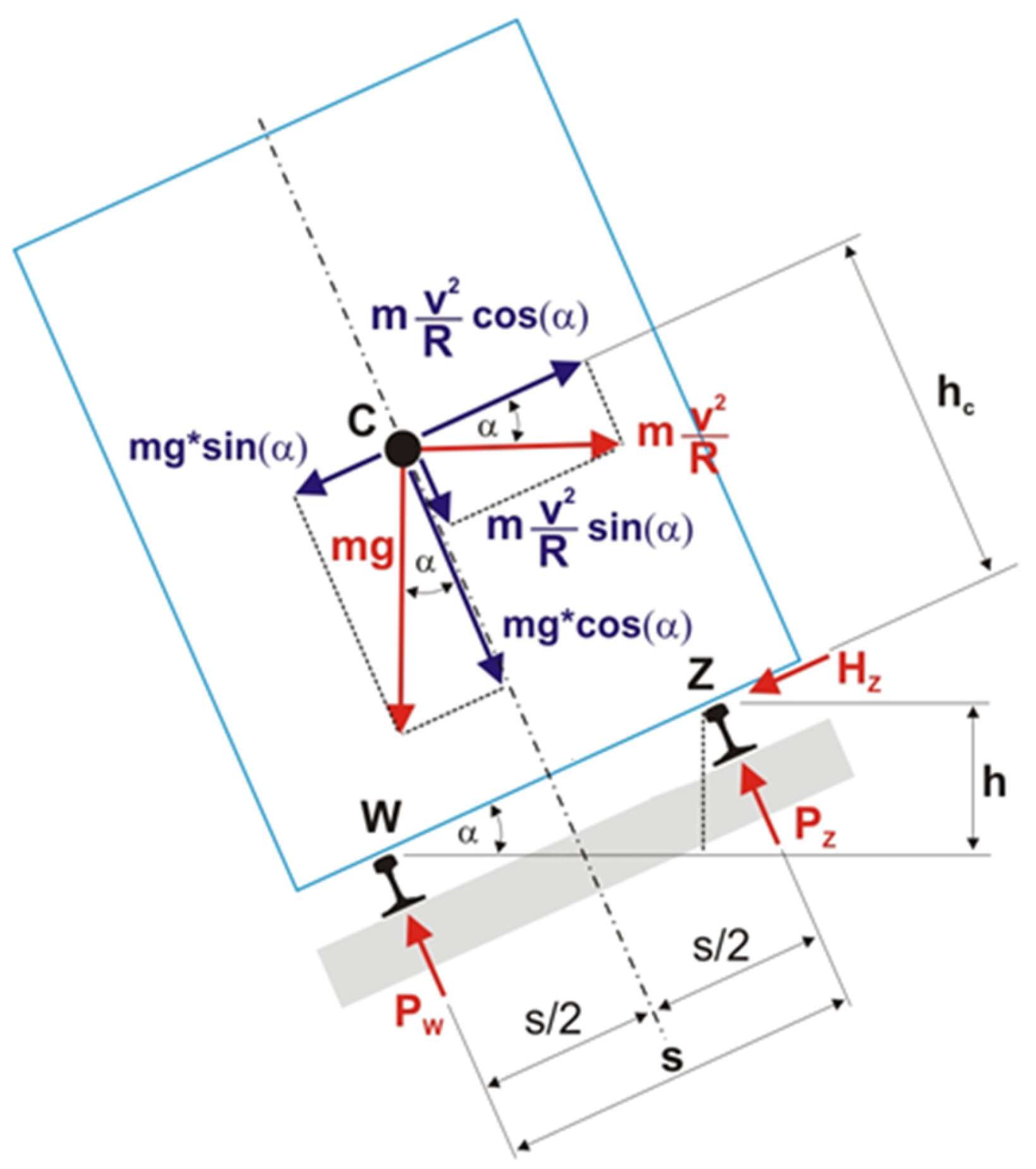
• The assumption is that the distribution of the sleeper mass along its axis is symmetric in relation to the centre of mass, and its rotations in relation to the centre of mass are small, i.e., the vertical displacement of the sleeper under the rail can be presented as a product of the rotation angle α and the distance between the cross-section directly under the rail from the sleeper’s centre of mass b (Figure 1).

2. Movement Equations and Their Solutions

2.1. Solution for Time-Invariable Forces

With the adopted assumptions, two systems of movement equations are formed:

• For the symmetric load:

$$\begin{array}{l}EI\frac{{\partial }^4{y}_{ra}}{\partial x^4}+N_t\frac{{\partial }^2{y}_{ra}}{\partial x^2}+m_r\frac{{\partial }^2{y}_{ra}}{\partial t^2}+c_r(\frac{\partial y_{ra}}{\partial t}-\frac{\partial y_{pa}}{\partial t})+k_r(y_{ra}-y_{pa})=q_{av}(x,t)\\ m_p\frac{{\partial }^2{y}_{pa}}{\partial t^2}+c_p\frac{\partial y_{pa}}{\partial t}+k_p{y}_{pa}=c_r(\frac{\partial y_{ra}}{\partial t}-\frac{\partial y_{pa}}{\partial t})+k_r(y_{ra}-y_{pa})\end{array}$$

(2)

• For the antisymmetric load:

$$\begin{array}{l}EI\frac{{\partial }^4{y}_{r\Delta }}{\partial x^4}+N_t\frac{{\partial }^2{y}_{r\Delta }}{\partial x^2}+m_r\frac{{\partial }^2{y}_{r\Delta }}{\partial t^2}+c_r(\frac{\partial y_{r\Delta }}{\partial t}-b\frac{\partial \varphi }{\partial t})+k_r(y_{r\Delta }-b\varphi )=\Delta q(x,t)\\ I_p\frac{{\partial }^2\varphi }{\partial t^2}+c_p{b}^2\frac{\partial \varphi }{\partial t}+k_p{b}^2\varphi =c_{r}b(\frac{\partial y_{r\Delta }}{\partial t}-b\frac{\partial \varphi }{\partial t})+k_{r}b(y_{r\Delta }-b\varphi )\end{array}$$

(3)

where

• y_rΔ—the rail displacement with an antisymmetric load (opposite signs for both rails) [m];
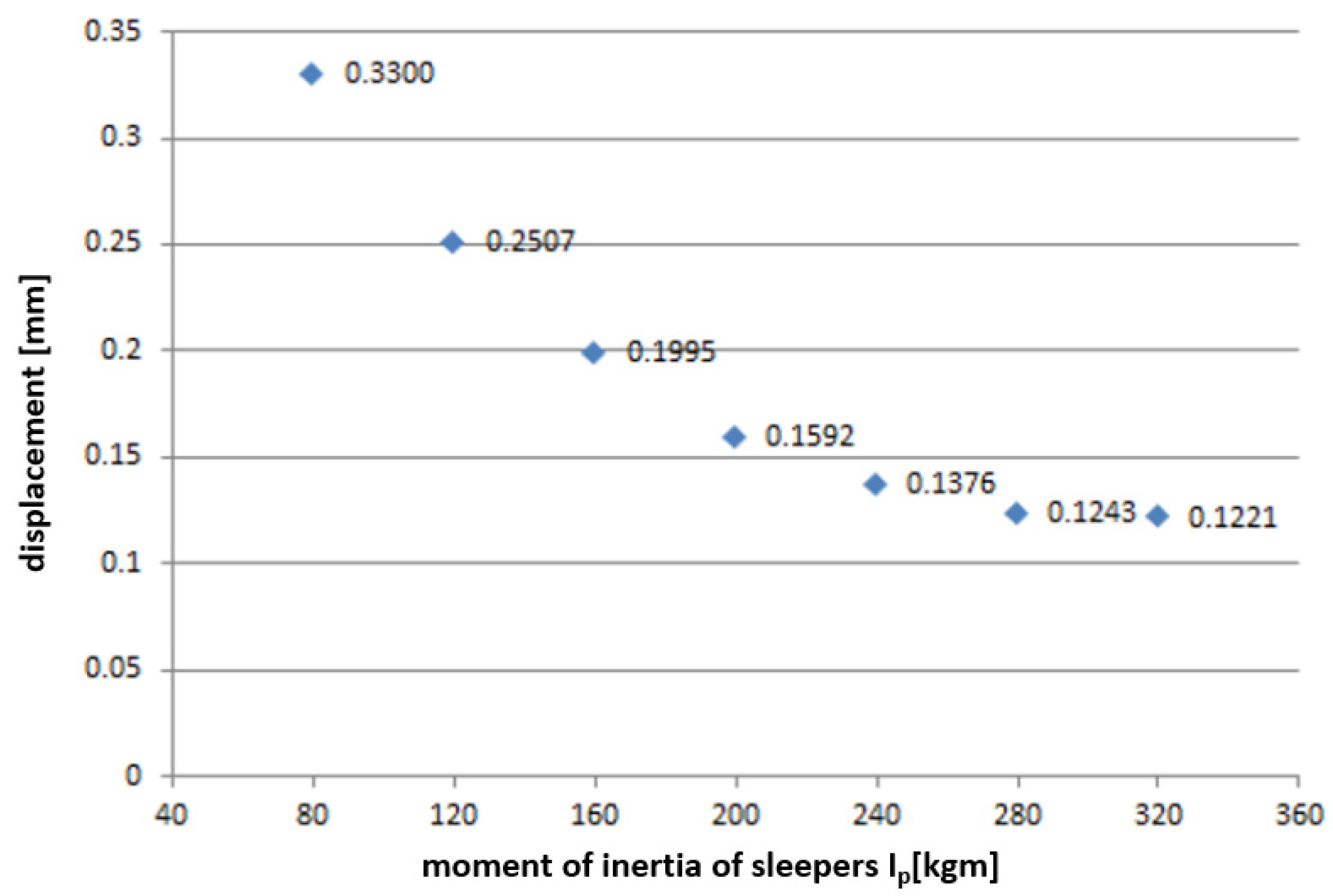
• I_p—the moment of inertia for individual sleepers (I_p = I_s/l_s, where I_s—the moment of inertia of a sleeper [kgm²], and l_s—the sleeper axis spacing along the track [m]);
• —Other symbols: as in Figure 1 and Figure 2.

The solutions for both load cases will be the sums of the solutions for the forces that are constant (non-oscillating—load symbol qⁿ) and time-variable (load symbol q^o). In a mobile coordinate system (η = y, ξ = x − vt,), where v—the constant train speed, the system of Equation (2) takes the following form for a system of non-time-variable forces:

$$\begin{array}{l}EI\frac{d^4{y}_{ra}}{d{\xi }^4}+(N_t+m_r{v}^2)\frac{d^2{y}_{ra}}{d{\xi }^2}-c_{r}v\frac{d{y}_{ra}}{d\xi }+k_r{y}_{ra}+c_{r}v\frac{d{y}_{pa}}{d\xi }-k_r{y}_{pa}=q_{av}^n(\xi )\\ m_p{v}^2\frac{d^2{y}_{pa}}{d{\xi }^2}-c_{p}v\frac{d{y}_{pa}}{d\xi }+k_p{y}_{pa}+c_{r}v\frac{d{y}_{ra}}{d\xi }-c_{r}v\frac{d{y}_{pa}}{d\xi }-k_r{y}_{ra}+k_r{y}_{pa}=0\end{array}$$

(4)

When marking the vertical displacement of a sleeper under the rail with an antisymmetric load with y_pΔ = φb, the system of Equation (3)—in a mobile coordinate system with a non-oscillating load—assumes the following form:

$$\begin{array}{l}EI\frac{d^4{y}_{r\Delta }}{d{\xi }^4}+(N_t+m_r{v}^2)\frac{d^2{y}_{r\Delta }}{d{\xi }^2}-c_{r}v\frac{d{y}_{r\Delta }}{d\xi }+k_r{y}_{r\Delta }+c_{r}v\frac{d{y}_{p\Delta }}{d\xi }-k_r{y}_{p\Delta }=\Delta q^n(\xi )\\ I_p\frac{v^2}{b^2}\frac{d^2{y}_{p\Delta }}{d{\xi }^2}-c_{p}v\frac{d{y}_{p\Delta }}{d\xi }+k_p{y}_{p\Delta }+c_{r}v\frac{d{y}_{r\Delta }}{d\xi }-c_{r}v\frac{d{y}_{p\Delta }}{d\xi }-k_r{y}_{r\Delta }+k_r{y}_{p\Delta }=0\end{array}$$

(5)

It is assumed that the load in Equation (4) is distributed throughout the length of the rail. Another assumption is that the function of the load distribution for every wheel of a vehicle has the form of a Gaussian function, i.e.,

$$\rho (\xi )=\frac{Q}{\sigma \cdot \sqrt{2\pi }}\cdot e^{-\frac{{(\xi -l_k)}^2}{2{\sigma }^2}};\xi \in [0,\lambda ];k=1,\dots ,N$$

(6)

where

Q—the static wheel load [N];

σ—the distribution parameter (its value should allow for the distribution of the load of a single wheel in the rail axis to correspond to the real distribution) [m];

l_k—the position of the wheel in relation to coordinate ξ = 0 [m];

λ—the assumed span of distribution (outside the [0, λ] interval, function ρ practically equals 0);

N—the number of analysed wheels of a vehicle.

Load functions are now transformed into Fourier series. The series factors, in a general case, i.e., with constant a₀, cosine components a_i, and sine components b_i, have the following form:

$$\begin{array}{l}{a}_0=\frac{NQ}{\lambda };\\ a_i=\frac{2Q}{\lambda }\cdot e^{-\frac{2{\pi }^2{\sigma }^2}{{\lambda }^2}}\cdot ({\displaystyle \sum _{k=1}^N\cos \frac{2\cdot \pi \cdot l_k\cdot i}{\lambda }});\\ b_i=\frac{2Q}{\lambda }\cdot e^{-\frac{2{\pi }^2{\sigma }^2}{{\lambda }^2}}\cdot \left({\displaystyle \sum _{k=1}^N\sin \frac{2\cdot \pi \cdot l_k\cdot i}{\lambda }}\right).\end{array}$$

(7)

Therefore, the load on the right side of the first equation in system (4) can be formulated as follows:

$$\begin{array}{l}{q}_{av}^n(\xi )=\frac{a_0}{2}+{\displaystyle \sum _{i=1}^{\infty }(a_i\cdot \cos {\mathsf{\Omega }}_i\xi +}{b}_i\cdot \sin {\mathsf{\Omega }}_i\xi );\\ \xi \in [0,\lambda ];{\mathsf{\Omega }}_i=\frac{2\pi \cdot i}{\lambda }\end{array}$$

(8)

It is assumed that the vertical displacements of the rail and sleeper can be presented in the form of a Fourier series in [0, λ], i.e.,

$$\begin{array}{l}{y}_{ra}(\xi )=\frac{y_{ra0}}{2}+{\displaystyle \sum _{i=1}^{\infty }(A_i\cdot \cos {\mathsf{\Omega }}_i\xi +}{B}_i\cdot \sin {\mathsf{\Omega }}_i\xi );\\ y_{pa}(\xi )=\frac{y_{pa0}}{2}+{\displaystyle \sum _{i=1}^{\infty }(C_i\cdot \cos {\mathsf{\Omega }}_i\xi +}{D}_i\cdot \sin {\mathsf{\Omega }}_i\xi );\\ \xi \in [0,\lambda ];{\mathsf{\Omega }}_i=\frac{2\pi \cdot i}{\lambda }\end{array}$$

(9)

Substituting the relationships (9) in the equation system (4), the algebraic equation system for unknown factors A_i, B_i, C_i, and D_i is obtained:

$$\begin{array}{l}{A}_i\left[EI{\mathsf{\Omega }}_i^4-(N_t+m_r{v}^2){\mathsf{\Omega }}_i^2+k_r\right]+B_i\left[-c_{r}v{\mathsf{\Omega }}_i\right]+C_i\left[-k_r\right]+D_i\left[c_{r}v{\mathsf{\Omega }}_i\right]=a_i\\ A_i\left[c_{r}v{\mathsf{\Omega }}_i\right]+B_i\left[EI{\mathsf{\Omega }}_i^4-(N_t+m_r{v}^2){\mathsf{\Omega }}_i^2+k_r\right]+C_i\left[-c_{r}v{\mathsf{\Omega }}_i\right]+D_i\left[-k_r\right]=b_i\\ A_i\left[-k_r\right]+B_i\left[c_{r}v{\mathsf{\Omega }}_i\right]+C_i\left[k_r+k_p-m_p{v}^2{\mathsf{\Omega }}_i^2\right]+D_i\left[-(c_r+c_p)v{\mathsf{\Omega }}_i\right]=0\\ A_i\left[-c_{r}v{\mathsf{\Omega }}_i\right]+B_i\left[-k_r\right]+C_i\left[(c_r+c_p)v{\mathsf{\Omega }}_i\right]+D_i\left[k_r+k_p-m_p{v}^2{\mathsf{\Omega }}_i^2\right]=0\end{array}$$

(10)

whereas the constants in Equation (9) are determined by the following formulas:

$$\begin{array}{l}{y}_{ra0}=a_0\left(\frac{1}{k_r}+\frac{1}{k_p}\right)\\ y_{pa0}=\frac{a_0}{k_p}\end{array}$$

(11)

The same method is used in the antisymmetric form of rail and sleeper vibrations with a time-invariable load. If we express the load in Equation (5) as a Fourier series, in the same interval [0, λ] as before (factors: c₀—constant, c_i—the amplitude of the cosine components, and d_i—the amplitude of the sine components):

$$\begin{array}{l}{\Delta }^{n}q(\xi )=\frac{c_0}{2}+{\displaystyle \sum _{i=1}^{\infty }(c_i\cdot \cos {\mathsf{\Omega }}_i\xi +}{d}_i\cdot \sin {\mathsf{\Omega }}_i\xi );\\ \xi \in [0,\lambda ];{\mathsf{\Omega }}_i=\frac{2\pi \cdot i}{\lambda }\end{array}$$

(12)

and also expressing the searched-for functions of rail vibrations in the form of a Fourier series in the same interval [0, λ], i.e.,

$$\begin{array}{l}{y}_{r\Delta }(\xi )=\frac{y_{r\Delta 0}}{2}+{\displaystyle \sum _{i=1}^{\infty }(E_i\cdot \cos {\mathsf{\Omega }}_i\xi +}{F}_i\cdot \sin {\mathsf{\Omega }}_i\xi );\\ y_{p\Delta }(\xi )=\frac{y_{p\Delta 0}}{2}+{\displaystyle \sum _{i=1}^{\infty }(G_i\cdot \cos {\mathsf{\Omega }}_i\xi +}{H}_i\sin {\mathsf{\Omega }}_i\xi );\\ \xi \in [0,\lambda ];{\mathsf{\Omega }}_i=\frac{2\pi \cdot i}{\lambda }\end{array}$$

(13)

the formulas necessary to solve the problem are obtained.

Differentiating Equation (13) and substituting the obtained relationships with Equation (12) in Equation (5), the algebraic equations system with unknowns E_i, F_i, G_i, and H_i is obtained:

$$\begin{array}{l}{E}_i\left[EI{\mathsf{\Omega }}_i^4-(N_t+m_r{v}^2){\mathsf{\Omega }}_i^2+k_r\right]+F_i\left[-c_{r}v{\mathsf{\Omega }}_i\right]+G_i\left[-k_r\right]+H_i\left[c_{r}v{\mathsf{\Omega }}_i\right]=c_i\\ E_i\left[c_{r}v{\mathsf{\Omega }}_i\right]+F_i\left[EI{\mathsf{\Omega }}_i^4-(N_t+m_r{v}^2){\mathsf{\Omega }}_i^2+k_r\right]+G_i\left[-c_{r}v{\mathsf{\Omega }}_i\right]+H_i\left[-k_r\right]=d_i\\ E_i\left[-k_r\right]+F_i\left[c_{r}v{\mathsf{\Omega }}_i\right]+G_i\left[(k_r+k_p)-I_p\frac{v^2}{b^2}{\mathsf{\Omega }}_i^2\right]+H_i\left[-(c_r+c_p)v{\mathsf{\Omega }}_i\right]=0\\ E_i\left[-c_{r}v{\mathsf{\Omega }}_i\right]+F_i\left[-k_r\right]+G_i\left[(c_r+c_p)v{\mathsf{\Omega }}_i\right]+H_i\left[(k_r+k_p)-I_p\frac{v^2}{b^2}{\mathsf{\Omega }}_i^2\right]=0\end{array}$$

(14)

and the constants in Equation (13) are determined by the following formulas:

$$\begin{array}{l}{y}_{r\Delta 0}=c_0\left(\frac{1}{k_r}+\frac{1}{k_p}\right)\\ y_{p\Delta 0}=\frac{c_0}{k_p}\end{array}$$

(15)

2.2. Solution for Oscillating Forces

Thus, a set of equations necessary to determine the response of the system with load by time-invariable forces has been obtained. In the case of oscillating forces with the provided wheel frequency ω in a mobile coordinate system, Equation (2) describing the system vibrations with a symmetric load of both rails has the following form:

$$\begin{array}{c}\begin{array}{l}EI\frac{{\partial }^4{y}_{ra}}{\partial {\xi }^4}+N_t\frac{{\partial }^2{y}_{ra}}{\partial {\xi }^2}+m_r(\frac{{\partial }^2{y}_{ra}}{\partial t^2}-2v\frac{{\partial }^2{y}_{ra}}{\partial t\partial \xi }+v^2\frac{{\partial }^2{y}_{ra}}{\partial {\xi }^2})+c_r(\frac{\partial y_{ra}}{\partial t}-v\frac{\partial y_{ra}}{\partial \xi }-\frac{\partial y_{pa}}{\partial t}+v\frac{\partial y_{pa}}{\partial \xi })+\\ +k_r(y_{ra}-y_{pa})=q_{av}^o(\xi ,t)\end{array}\\ \begin{array}{l}{m}_p(\frac{{\partial }^2{y}_{pa}}{\partial t^2}-2v\frac{{\partial }^2{y}_{pa}}{\partial t\partial \xi }+v^2\frac{{\partial }^2{y}_{pa}}{\partial {\xi }^2})+c_p(\frac{\partial y_{pa}}{\partial t}-v\frac{\partial y_{pa}}{\partial \xi })+k_p{y}_{pa}=\\ +c_r(\frac{\partial y_{ra}}{\partial t}-v\frac{\partial y_{ra}}{\partial \xi }-\frac{\partial y_{pa}}{\partial t}+v\frac{\partial y_{pa}}{\partial \xi })+k_r(y_{ra}-y_{pa})\end{array}\end{array}$$

(16)

The load in the first equation of system (16) can be formulated as follows:

$$q_{av}^o(\xi ,t)=q_{avc}(\xi )\cdot \cos \omega t+q_{avs}(\xi )\cdot \sin \omega t$$

(17)

where q_avc and q_avs are the cosine and sine components of the symmetric load.

The following form [16] is used to obtain the stationary solution of system (16):

$$\begin{array}{l}{y}_{ra}(\xi ,t)=Y_{rac}(\xi )\cdot \cos \omega t+Y_{ras}(\xi )\cdot \sin \omega t\\ y_{pa}(\xi ,t)=Y_{pac}(\xi )\cdot \cos \omega t+Y_{pas}(\xi )\cdot \sin \omega t\end{array}$$

(18)

When differentiating Equation (18), taking into consideration relationships (17), system (16) has the form of a system of four ordinary equations taking into consideration the cosine and sine components of the solutions of the following system:

$$\begin{array}{l}{L}_1(Y_{rac},Y_{ras},Y_{pac},Y_{pas},P)\cdot \cos \omega t=q_{avc}\cdot \cos \omega t\\ L_2(Y_{rac},Y_{ras},Y_{pac},Y_{pas},P)\cdot \sin \omega t=q_{avs}\cdot \sin \omega t\\ L_3(Y_{rac},Y_{ras},Y_{pac},Y_{pas},P)\cdot \cos \omega t=0\cdot \cos \omega t\\ L_4(Y_{rac},Y_{ras},Y_{pac},Y_{pas},P)\cdot \sin \omega t=0\cdot \sin \omega t\end{array}$$

(19)

where L₁–L₄—the linear operators Y_rac, Y_ras, Y_pac, and Y_pas of the functions and their derivatives; P—the vector of the model parameters (EI, m_r, N_t, k_r, etc., see Figure 2). For example, operator L₁ has the following form:

$$\begin{array}{l}{L}_1=EI\frac{d^4{Y}_{rac}}{d{\xi }^4}-m_r{\omega }^2{Y}_{rac}-2m_{r}v\omega \frac{d{Y}_{ras}}{d\xi }+(N_t+m_r{v}^2)\frac{d^2{Y}_{rac}}{d{\xi }^2}+c_r\omega Y_{ras}-c_{r}v\frac{d{Y}_{rac}}{d\xi }-\\ -c_r\omega Y_{pas}+c_{r}v\frac{d{Y}_{pac}}{d\xi }+k_r{Y}_{rac}-k_r{Y}_{pac}\end{array}$$

(20)

To solve system (19), the same method as before is adopted, i.e., both the cosine and sine components of loads q_avc and q_avs, as well as the unknown functions Y_rac, Y_ras, Y_pac, and Y_pas describing the vibrations of the rail and the sleeper with a symmetric time-variable load, are expressed in the form of a Fourier series in the interval [0, λ]:

$$\begin{array}{l}{q}_{avc}(\xi )=\frac{a_0}{2}+{\displaystyle \sum _{i=1}^{\infty }(a_i\cdot \cos {\mathsf{\Omega }}_i\xi +}{b}_i\cdot \sin {\mathsf{\Omega }}_i\xi );\\ q_{avs}(\xi )=\frac{c_0}{2}+{\displaystyle \sum _{i=1}^{\infty }(c_i\cdot \cos {\mathsf{\Omega }}_i\xi +}{d}_i\cdot \sin {\mathsf{\Omega }}_i\xi )\\ Y_{rac}(\xi )=\frac{Y_{ra01}}{2}+{\displaystyle \sum _{i=1}^{\infty }(A_i\cdot \cos {\mathsf{\Omega }}_i\xi +}{B}_i\cdot \sin {\mathsf{\Omega }}_i\xi );\\ Y_{ras}(\xi )=\frac{Y_{ra02}}{2}+{\displaystyle \sum _{i=1}^{\infty }(C_i\cdot \cos {\mathsf{\Omega }}_i\xi +}{D}_i\cdot \sin {\mathsf{\Omega }}_i\xi );\\ Y_{pac}(\xi )=\frac{Y_{pa01}}{2}+{\displaystyle \sum _{i=1}^{\infty }(E_i\cdot \cos {\mathsf{\Omega }}_i\xi +}{F}_i\cdot \sin {\mathsf{\Omega }}_i\xi );\\ Y_{pas}(\xi )=\frac{Y_{pa02}}{2}+{\displaystyle \sum _{i=1}^{\infty }(G_i\cdot \cos {\mathsf{\Omega }}_i\xi +}{H}_i\cdot \sin {\mathsf{\Omega }}_i\xi )\\ \xi \in [0,\lambda ];{\mathsf{\Omega }}_i=\frac{2\pi \cdot i}{\lambda }\end{array}$$

(21)

where—not to unnecessarily increase the number of symbols—the same symbols as in the case of the time-invariable load were used (i.e., a₀, a_i…. and then A_i, B_i, etc.). These values are of course different than the ones used previously in Formulas (8), (9), (12) and (13).

When differentiating relationships (22) and substituting them into (20), after reorganisation, a system of algebraic equations with unknown factors A_i–H_i is obtained:

$$\begin{array}{l}{A}_i\cdot P_1+B_i\cdot (-P_2)+C_i\cdot P_3+D_i\cdot (-P_4)+E_i\cdot P_5+F_i\cdot P_2+G_i\cdot (-P_3)+H_i\cdot P_6=a_i\\ A_i\cdot P_2+B_i\cdot P_1+C_i\cdot P_4+D_i\cdot P_3+E_i\cdot (-P_2)+F_i\cdot (-P_5)+G_i\cdot P_6+H_i\cdot (-P_3)=b_i\\ A_i\cdot (-P_3)+B_i\cdot P_4+C_i\cdot P_1+D_i\cdot (-P_2)+E_i\cdot P_3+F_i\cdot P_6+G_i\cdot (-P_5)+H_i\cdot P_2=c_i\\ A_i\cdot (-P_4)+B_i\cdot (-P_3)+C_i\cdot P_2+D_i\cdot P_1+E_i\cdot P_6+F_i\cdot P_3+G_i\cdot (-P_2)+H_i\cdot (-P_5)=d_i\\ A_i\cdot (-P_5)+B_i\cdot P_2+C_i\cdot (-P_3)+D_i\cdot P_6+E_i\cdot P_7+F_i\cdot (-P_8)+G_i\cdot P_9+H_i\cdot (-P_{10})=0\\ A_i\cdot (-P_2)+B_i\cdot (-P_5)+C_i\cdot P_6+D_i\cdot (-P_3)+E_i\cdot P_8+F_i\cdot P_7+G_i\cdot P_{10}+H_i\cdot P_9=0\\ A_i\cdot P_3+B_i\cdot P_6+C_i\cdot (-P_5)+D_i\cdot P_2+E_i\cdot (-P_9)+F_i\cdot P_{10}+G_i\cdot P_7+H_i\cdot (-P_8)=0\\ A_i\cdot P_6+B_i\cdot P_3+C_i\cdot (-P_2)+D_i\cdot (-P_5)+E_i\cdot (-P_{10})+F_i\cdot (-P_9)+G_i\cdot P_8+H_i\cdot P_7=0\\ \end{array}$$

(22)

where

$$\begin{array}{l}{P}_1=EI{\mathsf{\Omega }}_i^4-m_r{\omega }^2-(N_t+m_r{v}^2){\mathsf{\Omega }}_i^2+k_r\\ P_2=c_{r}v{\mathsf{\Omega }}_i\\ P_3=c_r\omega \\ P_4=2m_{r}v\omega {\mathsf{\Omega }}_i\\ P_5=k_r\\ P_6=0\\ P_7=-m_p{\omega }^2-m_p{v}^2{\mathsf{\Omega }}_i^2+k_r+k_p\\ P_8=(c_r+c_p)v{\mathsf{\Omega }}_i\\ P_9=(c_r+c_p)\omega \\ P_{10}=2m_{p}v\omega {\mathsf{\Omega }}_i\end{array}$$

(23)

The constants present in the relationships (21) are determined from the system of equations:

$$\begin{array}{l}{Y}_{ra01}\cdot (k_r-m_r{\omega }^2)+Y_{ra02}(c_r\omega )+Y_{pa01}(-k_r)+Y_{pa02}(-c_r\omega )=a_0\\ Y_{ra01}\cdot (-c_r{\omega }^2)+Y_{ra02}(k_r-m_r{\omega }^2)+Y_{pa01}(c_r\omega )+Y_{pa02}(-k_{hr})=c_0\\ Y_{ra01}\cdot (-k_r)+Y_{ra02}(-c_r\omega )+Y_{pa01}(k_r+k_p-m_p{\omega }^2)+Y_{pa02}(c_r\omega +c_p\omega )=0\\ Y_{ra01}\cdot (c_r\omega )+Y_{ra02}(-k_r)+Y_{pa01}(-c_p\omega -c_r\omega )+Y_{pa02}(k_r+k_p-m_p{\omega }^2)=0\end{array}$$

(24)

In reference to the antisymmetric load with a time-variable (oscillating) load, it is easy to notice that with the following substitution:

$$\begin{array}{l}{q}_{av}^o(\xi ,t):=\Delta q^o(\xi ,t);\\ y_{ra}=y_{r\Delta };\\ y_{pa}=y_{p\Delta };\\ m_p=\frac{I_p}{b^2}\end{array}$$

(25)

an equation is obtained, which—from the point of view of its structure—is identical to (16). Therefore, both the method of solving and the obtained formulas, with the substitution of (25), will be identical in reference to Formulas (21) and (22), in which the symbols of the functions describing the spatial constants and the cosine and sine components of the bending curve and the load curve should be changed (the “a” index should be changed to “Δ” in the components of the rail and sleeper displacement and the “av” index to “Δ” in the case of load components).

2.3. Solution for Track Response as a Two-Layer Structure

The method of solving the track response as a two-layer structure, with an uneven rail load and the assumption of sleeper rotation as stiffblocks, is as follows:

• For the given functions of rails loads q₁ and q₂, determine the symmetric q_av and antisymmetric Δq components of the load according to Formula (1).
• Isolate from every form of the load a time-invariable component and a time-variable component, i.e.,

$$\begin{array}{l}{q}_{av}=q_{av}^n+q_{av}^o\\ \Delta q=\Delta q^n+\Delta q^o\end{array}$$

(26)

3.

Using symbol y_r1 for the rail displacement for which the quasi-static load (time-invariable) is greater than for the other rail, which will be designated as y_r2, respectively, the sleeper displacement under both rails, y_p1 and y_p2, determine them, using Formulas (8)–(15):

$$\begin{array}{l}{y}_{r1}\left(q_{av}^n\right)=y_{ra}\left(q_{av}^n\right)+y_{r\Delta }(\Delta q^n);\\ y_{r2}\left(q_{av}^n\right)=y_{ra}\left(q_{av}^n\right)-y_{r\Delta }(\Delta q^n);\\ y_{p1}\left(q_{av}^n\right)=y_{pa}\left(q_{av}^n\right)+y_{p\Delta }(\Delta q^n);\\ y_{p2}\left(q_{av}^n\right)=y_{pa}\left(q_{av}^n\right)-y_{p\Delta }(\Delta q^n)\end{array}$$

(27)

4.

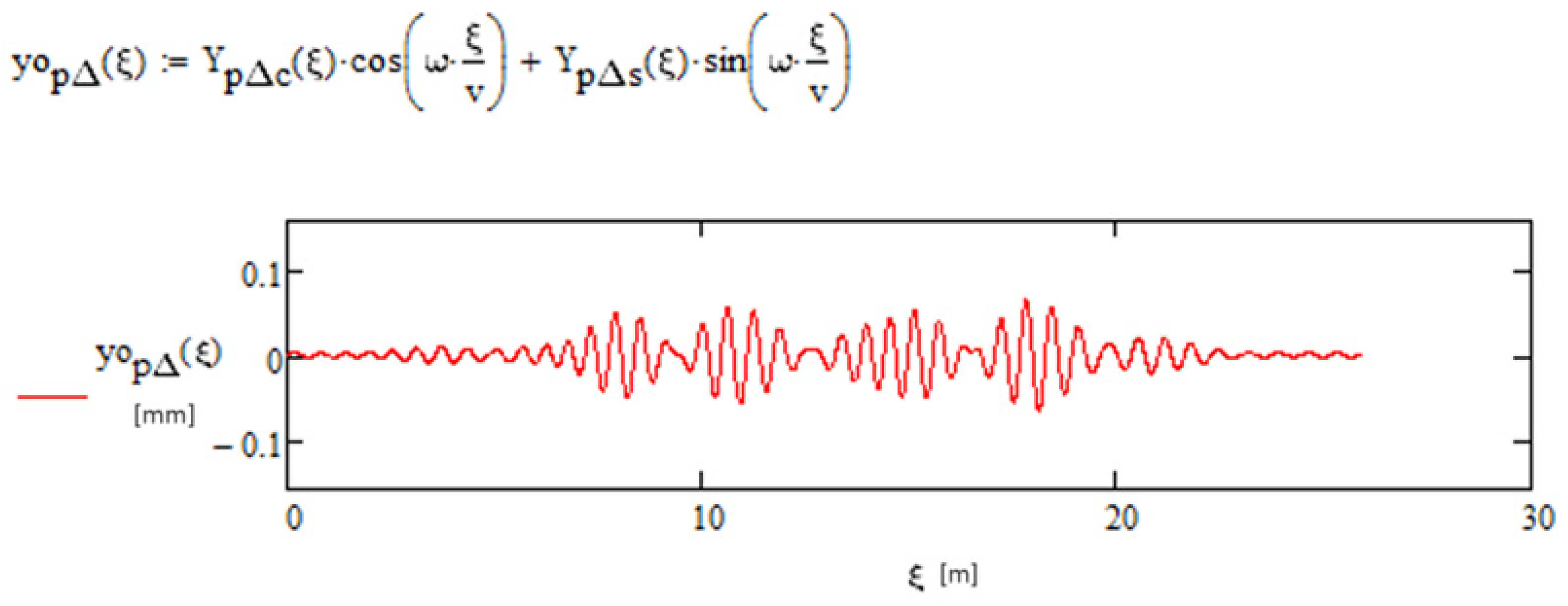
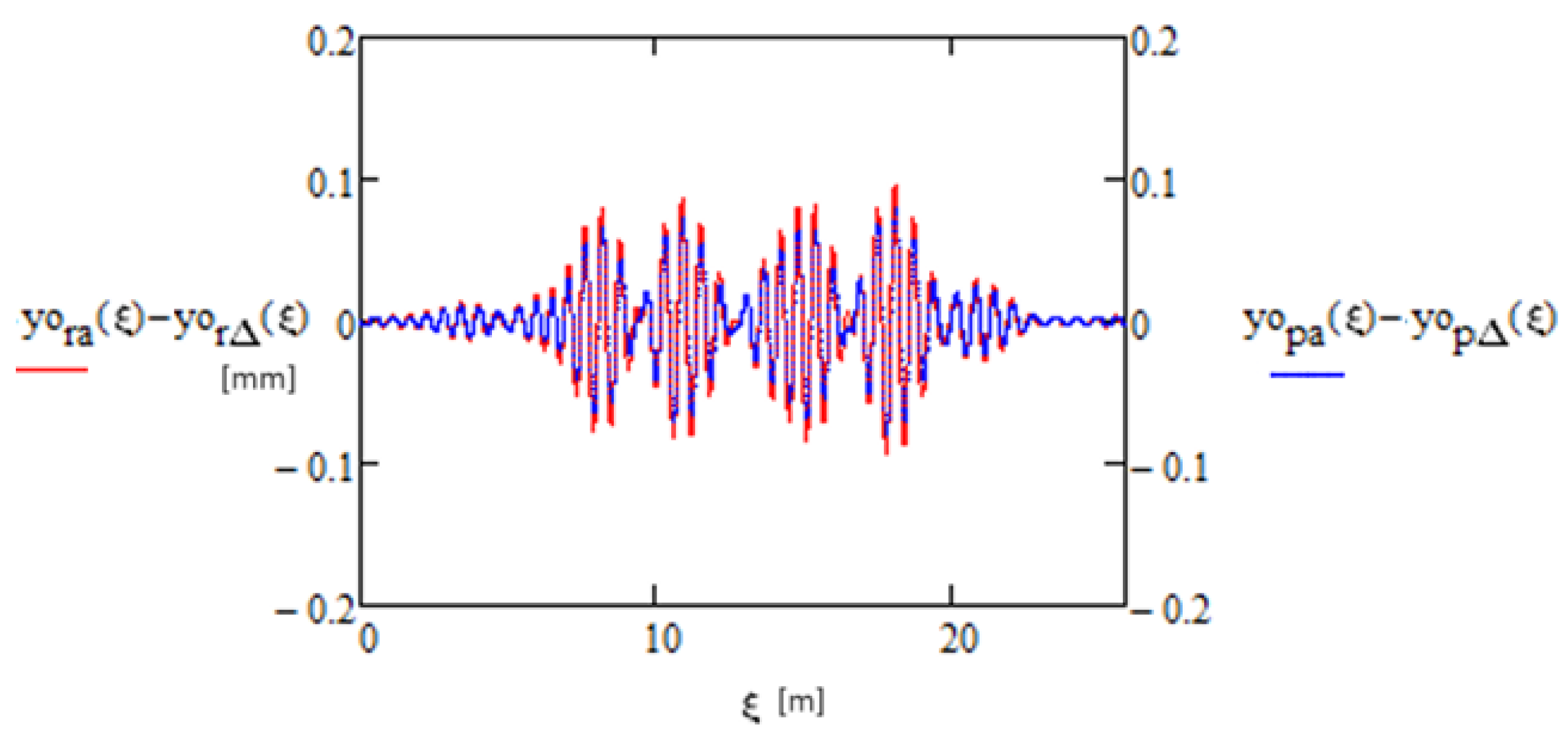
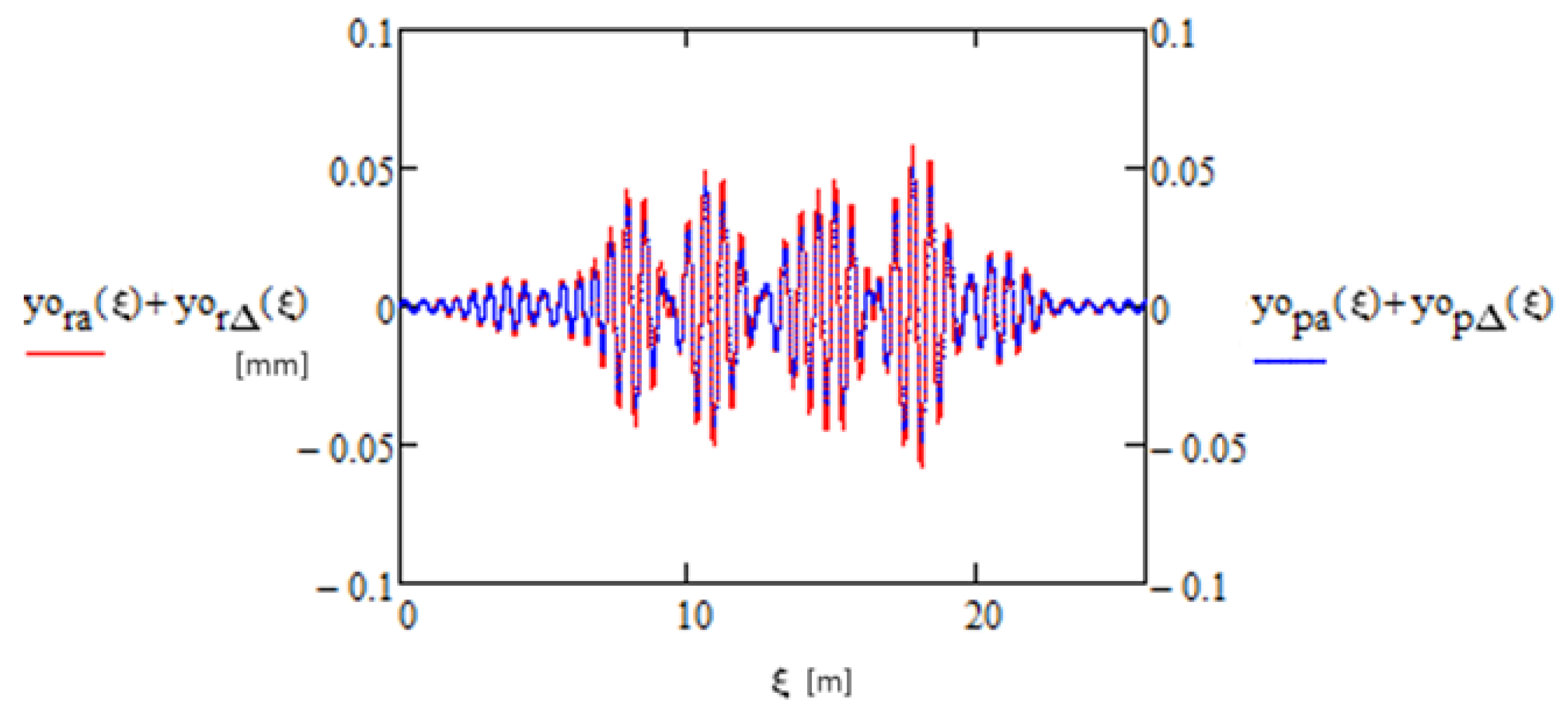
Using Formulas (17)–(24), determine the rail displacement and sleeper displacement for the time-variable load q^o (oscillating with a given frequency ω):

$$\begin{array}{l}{y}_{r1}\left(q_{av}^o\right)=y_{ra}\left(q_{av}^o\right)+y_{r\Delta }(\Delta q^o);\\ y_{r2}\left(q_{av}^o\right)=y_{ra}\left(q_{av}^{o)}\right)-y_{r\Delta }(\Delta q^o);\\ y_{p1}\left(q_{av}^o\right)=y_{pa}\left(q_{av}^o\right)+y_{p\Delta }(\Delta q^o);\\ y_{p2}\left(q_{av}^o\right)=y_{pa}\left(q_{av}^o\right)-y_{p\Delta }(\Delta q^o)\end{array}$$

(28)

5.

If a variable load is polyharmonic (more than one frequency ω), the calculations expressed with Formula (27) should be repeated as many times for as many harmonic components of time-variable force there are.

6.

The total rail displacements and total sleeper displacements are a sum of these displacements resulting from the constant load (Formula (27)) and variable load (Formula (26)), whereas—in the case of a polyharmonic load, where there are m harmonic components—Formula (28) should be applied m times, and the results should be added.

3. Calculation Examples

The calculations of the track response according to the adopted model were performed using Mathcad Prime 3.1 software. The calculations for the time-invariable load and the calculations for the time-variable load were performed separately. The obtained results for both rails (with higher and lower loads) and sleepers (with higher and lower loads) were added in MS Excel 2021 software, and the results were presented in graphic form.

3.1. Introductory Notes

A simplified model of vehicle movement in a curve was analysed (Figure 3, based on [22]). The simplification is based on the fact that we treated the vehicle as a stiff element, and, additionally, the rotation resulting from the deformation of the suspension springs was ignored. The reactions transferred through the vehicle wheels to both rails constituted—for a given value of the cant h, curve radius R, centre of mass position in relation to the rail heads h_c, and the vehicle speed v—constant rail loads different for both rails (symbols in Figure 3, P_z and P_w).

The vertical reactions P_z and P_w and a horizontal reaction H_z were determined using system equilibrium equations. These are expressed by the following formulas:

$$\begin{array}{c}{\mathrm{H}}_{\mathrm{z}}=\mathrm{m}\frac{{\mathrm{v}}^2}{\mathrm{R}}\mathrm{*}\cos \mathsf{\alpha }-\mathrm{m}\mathrm{g}\mathrm{*}\sin \mathsf{\alpha }\\ P_z=m\cdot \left[g\cdot \left(\frac{1}{2}\cos \alpha -\frac{h_c}{s}\sin \alpha \right)+\frac{v^2}{R}\cdot \left(\frac{1}{2}\sin \alpha +\frac{h_c}{s}\cos \alpha \right)\right]\\ P_w=m\cdot \left[g\cdot \left(\frac{1}{2}\cos \alpha +\frac{h_c}{s}\sin \alpha \right)+\frac{v^2}{R}\cdot \left(\frac{1}{2}\sin \alpha -\frac{h_c}{s}\cos \alpha \right)\right]\\ H_z=m\cdot \frac{v^2}{R}\cdot \cos \alpha -mg\cdot \sin \alpha \end{array}$$

(29)

The trigonometric functions present in the formulas were determined from the following geometrical relationships:

$$\sin \alpha =\frac{h}{s},\mathit{cos}\alpha =\frac{b}{s},h^2+b^2=s^2,b=\sqrt{s^2-h^2},\cos \alpha ={\sqrt{1-\left(\frac{h}{b}\right)}}^2$$

(30)

In reference to the time-variable load—for the given vehicle axis configuration—multiple instances of geometrical unevenness of the rail were assumed. It was assumed—similarly to article [11]—that rail vibrations are driven by forces resulting from vertical displacements of the wheel along the unevenness for the given stiffness of the wheel–rail contact. This means that the force amplitude will be equal to the amplitude of the unevenness r_o multiplied by the stiffness of the contact between the wheel and rail k_c, while the frequency of force changes will be based on the length of the wave of the unevenness L_r and the given train speed v. If a single wave of unevenness described by the equation:

$$r(x)=r_0\cdot \cos \frac{2\pi x}{L_r}$$

(31)

is analysed, the driving force for the first wheel of the vehicle will have the following form:

$$P(t)=r_0\cdot k_c\cos \frac{2\pi vt}{L_s}=\Delta P\cdot \cos \omega t$$

(32)

where ΔP = r_ok_c, ω = 2πv/L_r.

The driving force for the following wheels will depend on the configuration of the train axles in reference to the given length L_r, which has been described in article [11].

3.2. Adopted Parameters

During the analyses, basic parameters were adopted for the track built, respectively, of the following:

• A 60 E1 rail, as the Euler–Bernoulli beam: E = 2.1 × 10⁸ N/m², I = 3055 × 10⁻⁸ m⁴, m_r = 60 kg.
• PS94 concrete sleepers, as stiffblocks: A = 0.68/2 m², m_p = 267 kg/m.
• An elastic fastening system with elastic-dampening parameters (rail–sleeper bonds): k_r = 9.1 × 10⁷ N/m, c_r = 3950 Ns/m.
• The foundation under the sleepers with elastic-dampening parameters (sleeper–foundation bonds): k_p = 8.8 × 10⁷ N/m², c_p = 49,000 Ns/m².
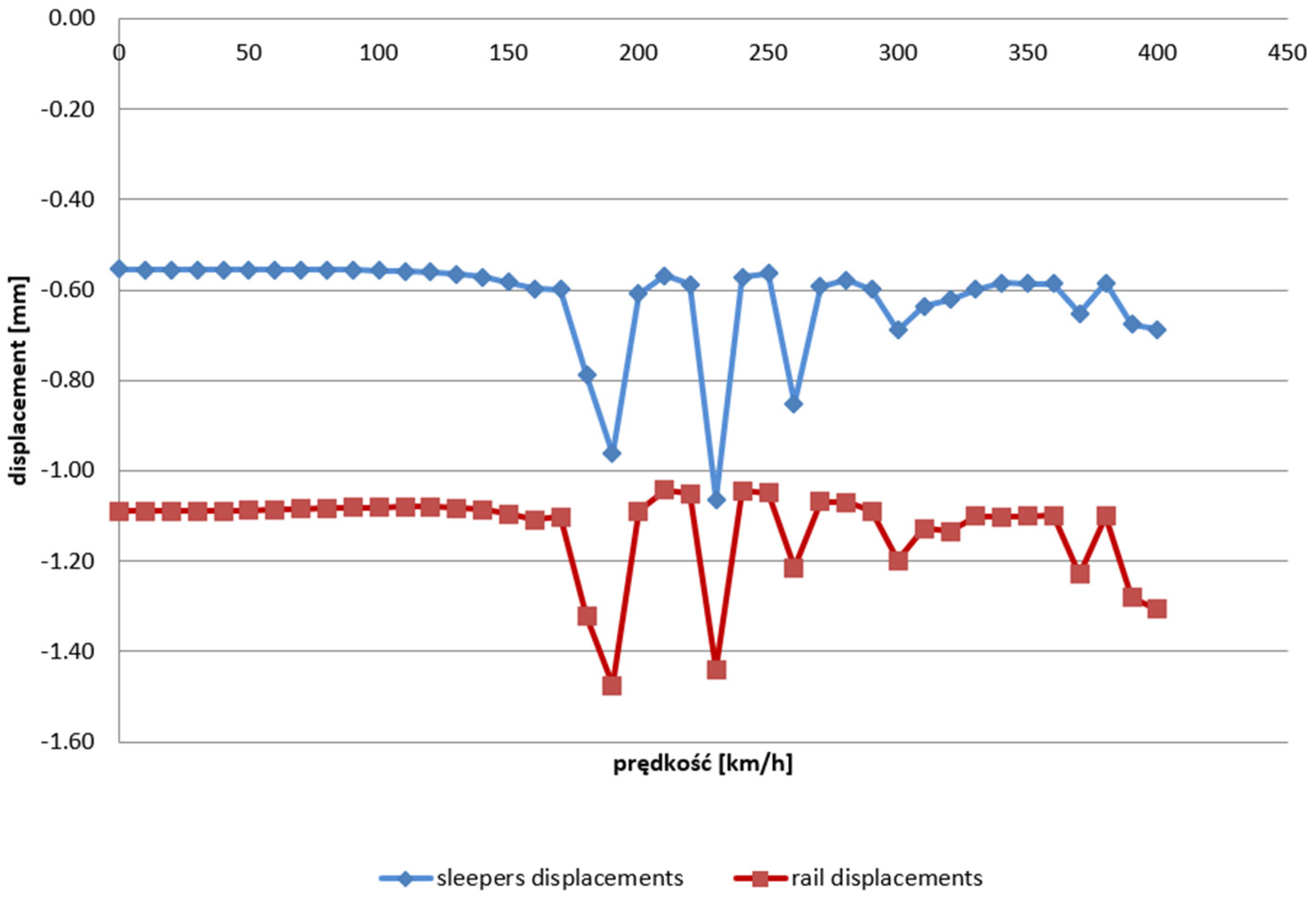
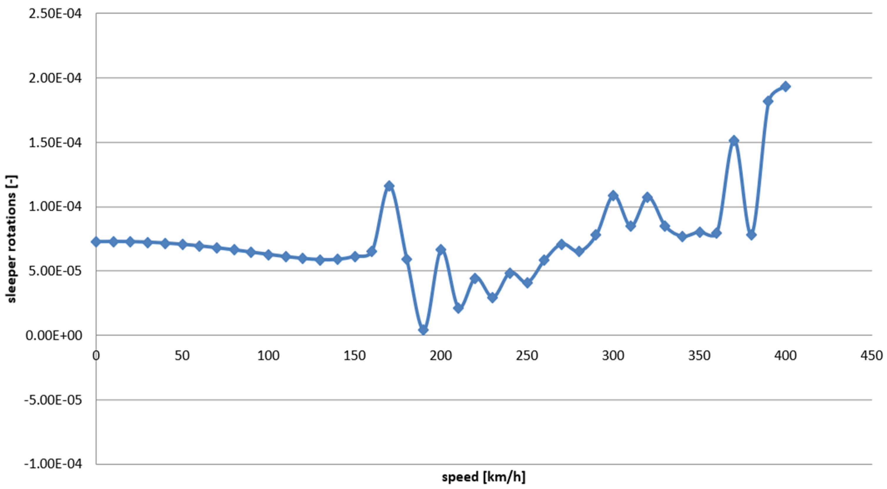
• A variable parameter of the train speed v (force system) was adopted, which was changing from 0 km/h to 400 km/h, leading to a change in the wheel loads on the internal and external rails (higher and lower loads) with the given constant curve radius R = 5580 m, cant h_p = 100 mm, and wheel load on the axis Q = 160 kN. The values of the forces influencing the internal track P_w (with lower load) and the external track P_z (with higher load) were calculated with Formula (29), and they are, respectively, P_w = 64.1 kN and P_z = 94.4 kN. Examples of the calculations for the rails and sleepers for the speed v = 170 km/h are presented in the following chapters.

After determining the forces, the axle spacing corresponding to the actual spacing of the middle bogies EMU 250 Pendolino (Alstom, Warsaw, Poland) was assumed. Additionally, 8-m sections (the distance for which the track response is different than 0; 25.9 m in total) as well as the number of terms of the Fourier series expansion n = 3000 were adopted.

When describing the time-variable load, it was assumed, in accordance with [22], that the loading forces originate from the contact of the wheel and rail, which can be expressed with the formula ∆P = s₀ × k_c, where s₀—the displacement from the unevenness equal to 1 [µm] and k_c—the stiffness of the wheel–rail contact equal to 1.1 × 10⁶ [kN/m]. The unevenness s₀ was assumed to be the rail bending between sleepers, where the unevenness length L_s is equal to the sleeper spacing, which in this case is 0.6 m.

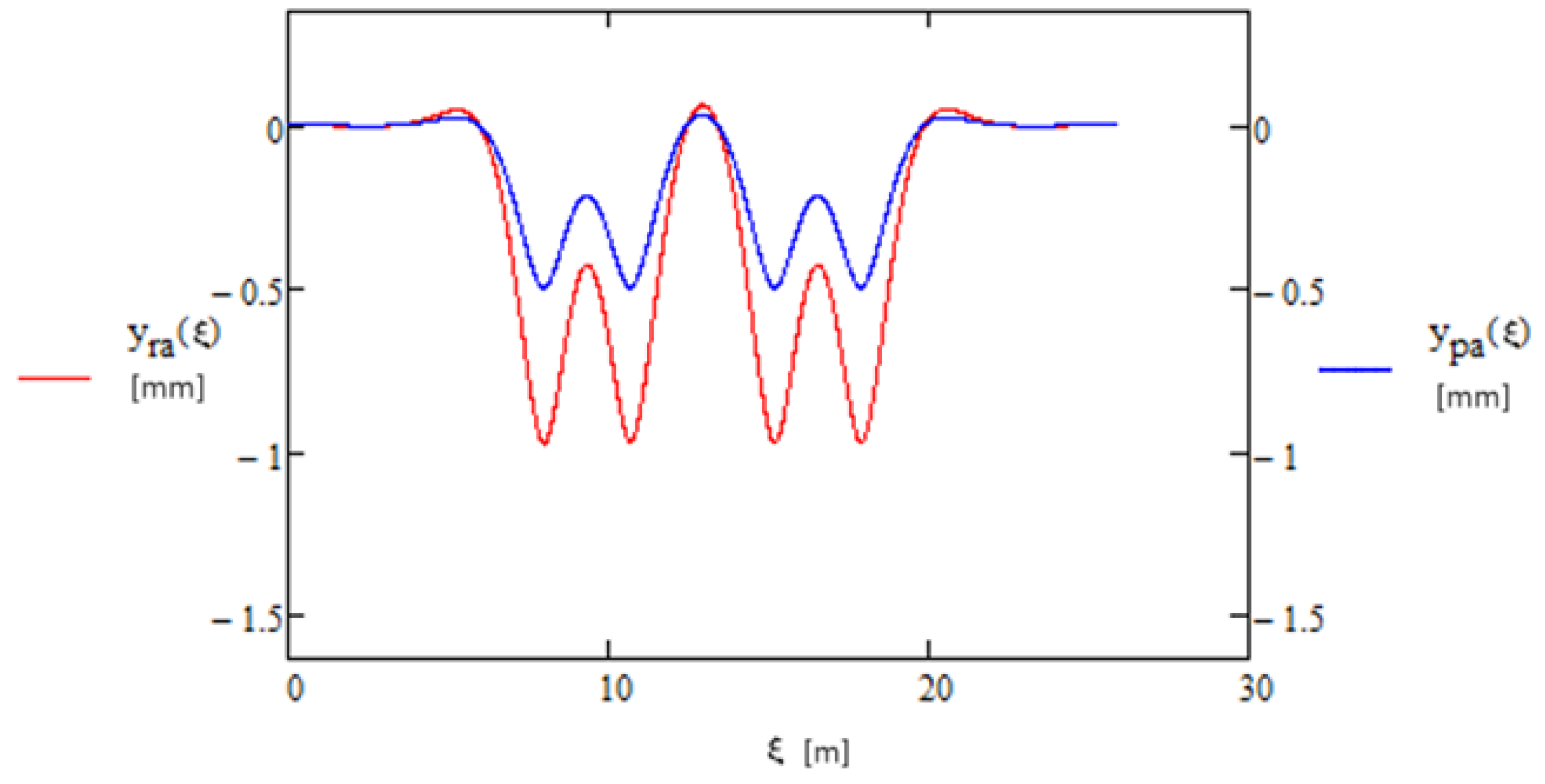
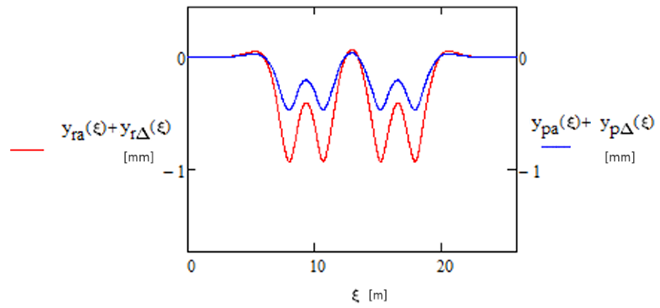
3.3. Example of Determining Rail and Sleeper Displacements with Time-Invariable Load

Figure 4 presents the bending of the rails and sleepers for the symmetric component of the time-invariable load for the speed v = 170 km/h. The obtained graph of the rail and sleeper bending is, as assumed, symmetric. The ends of the graph equal 0, which also confirms the assumptions.

Figure 5 presents the bending of the rails and sleepers for the antisymmetric component of the time-invariable load for the speed v = 170 km/h. For this purpose, it was necessary to determine the moment of inertia of a sleeper distributed over one running metre of track in relation to its middle axis. This parameter was obtained by dividing the sleeper into slices of 0.005 m with different cross-sections and calculating for them other moments of inertia.

The next step was to add the symmetric and antisymmetric components for both rails. Figure 6 presents the bending of the rails and sleepers with higher loads for the time-invariable load component for v = 170 km/h, whereas Figure 7 presents the bending of the rails and sleepers with lower loads for the time-invariable load component for v = 170 km/h.

When comparing Figure 4 and Figure 5, the bending of the rail with a lower load, y_r1(qⁿ_av) = 0.93 [mm], and with a higher load, y_r2(qⁿ_av) = 1.02 [mm], are obtained, with the latter value higher by nearly 9%. In the case of sleepers, the difference is even higher, and the displacements differ by over 11%, y_p1(qⁿ_av) = 0.47 [mm] and y_p2(qⁿ_av) = 0.53 [mm], which allows for concluding that sleeper rotation has occurred.

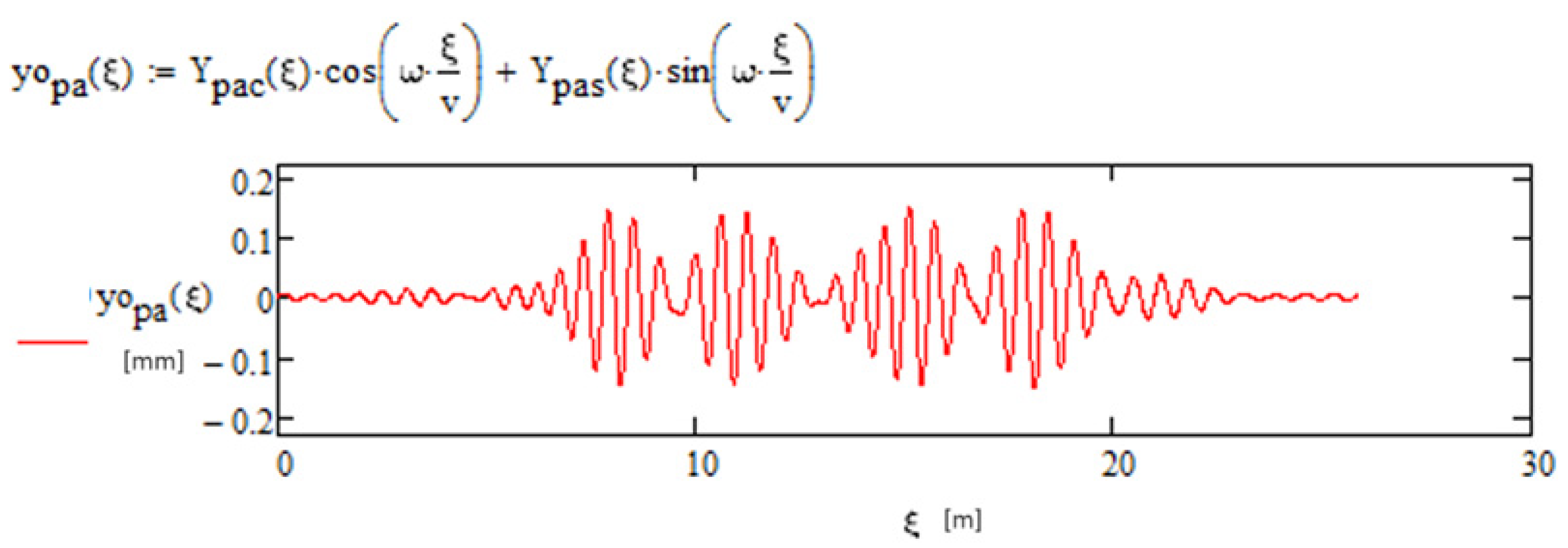
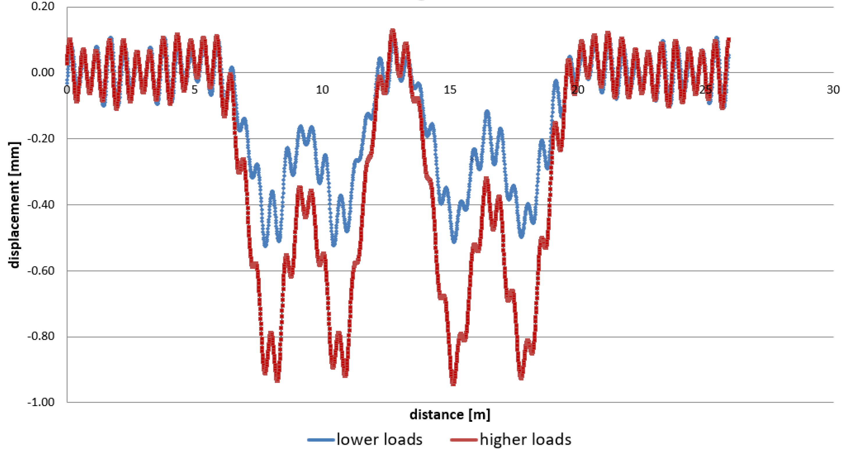
3.4. Example of Determining Rail and Sleeper Displacements with Time-Variable Load

Figure 8 presents the rail displacement, whereas Figure 9 shows the sleeper displacements caused by the time-variable symmetric load for v = 170 km/h and the rail unevenness up to s₀ = 10 × 10⁻⁶ m.

Figure 10 and Figure 11 present the rail and sleeper displacements for the antisymmetric part of the time-variable load. When performing the calculations, the moment of inertia of one-half of a sleeper per one metre and the quadrupled force ∆q⁰ = 2 × k_c × s₀ were taken into consideration.

After adding the symmetric and antisymmetric parts of the time-variable load, the results of the rail and sleeper bending for every rail were obtained. Figure 12 and Figure 13 present the obtained results for the rails with higher and lower loads, respectively, for v = 170 km/h.

When analysing the presented example, it can be concluded that the rail and sleeper displacements in both cases are similar, whereas the displacement for the rail and sleeper with a higher load (the applied load is 4 times higher) is twice as high.

4. Analysis of the Influence of Variable Parameters

In accordance with the outline described above, a series of analyses was performed for the following variable parameters: the speed v ∈ (0;400) and the individual moment of inertia of the sleepers I_p. Displacement graphs and tables with the maximum bending for both rails, as well as tangent α of the sleeper rotation, were obtained.

4.1. Speed

Figure 14 and Figure 15 present the consolidated relationships between the rail and sleeper bending, respectively, with higher and lower loads and the changing speed in the assumed range from v = 0 km/h to v = 400 km/h.

When comparing the bending of rails/sleepers with higher loads, it was noticed that along with an increasing speed, the linear bending increases as well. However, the bending of the rails/sleepers with lower loads takes place in a way that is difficult to describe. The displacements presented in Figure 15 decrease at the end of the graph. Initially, the results were interpreted as the track becoming more stiff due to the speed; however, after determining the bending of the rails/sleepers with higher loads, for which this phenomenon does not appear, the obtained results can be interpreted as the influence of sleeper rotation on bending (greater unloading of one of the rails), which appeared for the highest speeds. After superimposing sleeper bending for both rails, a graph of sleeper rotation for a given speed is obtained. Figure 16 presents the displacement of the sleepers under rails resulting from sleeper rotation for a hypothetical speed v = 300 km/h.

With the assumption that the rotation angles are low, the tangent is equal to the sleeper rotation angle α under the rail support points. Figure 17 presents tanaα related to the changing speed.

The aforementioned “exceptions” related to the linear graph of the rail and sleeper displacements present in the consolidated graphs, i.e., cases of a sudden increase in bending, for both rails appeared with the following speed values: v = 190 km/h, v = 230 km/h, v = 260 km/h, and v = 330 km/h. This graph of the rail/sleeper bending in these cases, both for the rails with a lower and higher load, is interpreted as the track resonance effect.

4.2. Influence of Sleeper’s Moment of Inertia

The individual moment of inertia for a sleeper was obtained by dividing the sleeper into slices of 0.005 m with different cross-sections and calculating for them I_s—the moment of inertia in accordance with the definition I_s = mr², where m is the slice mass and r is the distance between the middle of a slice to the sleeper axis. For example, for one-half of the PS94 sleeper, (Polish solution) (Plastwil, Ujście, Poland) the following results were obtained: I_s = 96.74 kgm² and I_p = 161.24 kgm. The calculations presented in the sections above were performed for an individual moment of inertia of the sleeper I_p = 161.23 kgm. To show the influence of parameter I_p, a section from I_p = 80 kgm—half of the actual value—to I_p = 320 kgm—twice the actual value—was adopted, with increments every 40 kgm. These values do not represent accurately other types of sleepers; however, they can be assigned to sleepers lighter or heavier than PS94. Figure 18 presents the sleeper displacement under the rails resulting from the sleeper rotation for speed v = 300 km/h and I_p = 80 kgm.

After performing a series of analyses for individual I_p values, it should be concluded that the increase in an individual moment of inertia of a sleeper leads to a reduction in the rotation effect. The quadruplication of the individual moment of inertia causes nearly a triple reduction in the displacements of the sleeper ends. Figure 19 presents the influence of an individual moment of inertia of a sleeper on its rotation with constant speed.

5. Summary and Conclusions

An original analytical model of a railway, taking into consideration sleeper rotations as stiffblocks, was presented in this article. In movement equations, an uneven load of rails was considered, which is present in curves with a speed different than the one with which the cant compensates for the lateral force and reduces the force system to one that is perpendicular to the straight line connecting the rail heads. This case is also present with the variable unevenness of the rolling surfaces of both rails.

The presented model significantly expands the scope of knowledge regarding an analytical description of the dynamic phenomena in a railway, specifically in reference to horizontal irregularities.

The broad scope of the parametric analysis of the model has revealed a significant influence of train speed on the diversity of sleeper displacement resulting from their rotations, as well as a significant influence of the moment of inertia on the parameters describing sleeper rotation.

Further analyses should be oriented on broadening the scope of variable parameters of the analysed model (non-uniform instances of unevenness of both rails; different track parameters, including the stiffness of fastening systems; etc.).

The model should also be improved by taking into consideration, e.g., asymmetric properties of a sleeper in relation to its centre of mass, which will enable the mitigation of the results of an uneven track load in horizontal irregularities.

References

1. Sysyn, M.; Nabochenko, O.; Kovalchuk, V. Experimental investigation of the dynamic behavior of railway track with sleeper voids. Railw. Eng. Sci. 2020, 28, 290–304. [Google Scholar] [CrossRef]
2. Sysyn, M.; Przybyłowicz, M.; Nabochenko, O.; Kou, L. Identification of Sleeper Support Conditions Using Mechanical Model Supported Data-Driven Approach. Sensors 2021, 21, 3609. [Google Scholar] [CrossRef] [PubMed]
3. Timoshenko, S. Method of analysis of static and dynamic stresses in rail. In Proceedings of the 2nd International Congress on Applied Mechanics, Zurich, Switzerland, 12–17 September 1926; pp. 407–418. [Google Scholar]
4. Basiewicz, T. Nawierzchnia Kolejowa na Podkładach Betonowych; WKiŁ: Warsaw, Poland, 1969. [Google Scholar]
5. Czyczuła, W. Analiza Wpływu Drgań Nawierzchni Kolejowej na Deformacje Podsypki. Ph.D. Thesis, Politechnika Krakowska im. Tadusza Kościuszki, Krakow, Poland, 1984. [Google Scholar]
6. Czyczula, W.; Kozioł, P.; Blaszkiewicz, D. On the equivalence between static and dynamic railway track response and on the Euler-Bernoulli and Timoshenko beams analogy. Shock. Vib. 2017, 2017, 2701715. [Google Scholar] [CrossRef]
7. Fryba, L. Vibration of Solids and Structures under Moving Loads; Noordhoff: Groningen, The Netherlands, 1972. [Google Scholar]
8. Koziol, P. Nonlinear response of railway track subjected to a moving train. In Proceedings of the ICEDYN 2015 International Conference on Structural Engineering Dynamics, Lagos, Algarve, Portugal, 22–24 June 2015; Maia, N.M.M., Neves, M.M., Sampaio, R.P.C., Eds.; paper K03. Instituto de Engenharia Mecânica: Lisabon, Portugal; Porto, Portugal, 2015; ISBN 978-989-96276-9-7. [Google Scholar]
9. Bogacz, R. Dynamics of continuous systems subjected to traveling loads. Appl. Mech. Mater. 2009, 9, 509–516. [Google Scholar] [CrossRef]
10. Kargarnovin, M.H.; Younesian, D.; Thompson, D.J.; Jones, C.J.C. Response of beams on nonlinear viscoelastic foundations to harmonic moving loads. Comput. Struct. 2005, 83, 1865–1877. [Google Scholar] [CrossRef]
11. Czyczula, W.; Koziol, P.; Kudla, D.; Lisowski, S. Analytical evaluation of track response in vertical direction due to moving load. J. Vib. Control. 2017, 23, 2989–3006. [Google Scholar] [CrossRef]
12. Sołkowski, J. The Transition Effect in Rail Tracks; Monografia 435; Politechnika Krakowska im. Tadeusza Kościuszki: Krakow, Poland, 2013. [Google Scholar]
13. Koziol, P.; Neves, M.M. Multilayered infinite medium subject to a moving load: Dynamic response and optimization using coiflet expansion. Shock. Vib. 2012, 19, 1009–1018. [Google Scholar] [CrossRef]
14. Zhai, W.; Xia, H.; Cai, C.; Gao, M.; Li, X.; Guo, X.; Zhang, N.; Wang, K. High-speed train-track-bridge dynamic interactions—Part I: Theoretical model and numerical simulation. Int. J. Rail Transp. 2013, 1, 3–24. [Google Scholar] [CrossRef]
15. Zhai, W.; Xia, H.; Cai, C.; Gao, M.; Li, X.; Guo, X.; Zhang, N.; Wang, K. High-speed train-track-bridge dynamic interactions—Part II: Experimental validation and engineering application. Int. J. Rail Transp. 2013, 1, 25–41. [Google Scholar] [CrossRef]
16. Bogacz, R.; Krzyżyński, T. O Belce Bernoulliego-Eulera Spoczywającej na Lepkosprężystym Podłożu Poddanej Działaniu Ruchomego Oscylacyjnego Obciążenia; Raport 38; Prace IPPT-PAN: Warsaw, Poland, 1986. [Google Scholar]
17. Ferrara, R.; Leonardi, G.; Jourdan, F. A Two-Dimansional Numerical Model to Analyse the Critical Velocity of High Speed Infrastructure. In Proceedings of the XIV-th International Conference on Civil, Structural and Environmental Engineering Computing, Cagliari, Sardinia, Italy, 3–6 September 2013. [Google Scholar]
18. Kerr, A.D. The continuously supported rail subjected to axial force and moving load. Int. J. Mech. Sci. 1972, 14, 71–78. [Google Scholar] [CrossRef]
19. Koziol, P.; Mares, C. Wavelet approach for vibration analysis of fast moving load on a viscoelastic medium. Shock. Vib. 2010, 17, 461–472. [Google Scholar] [CrossRef]
20. Hryniewicz, Z.; Koziol, P. Wavelet approach for analysis of dynamic response of Timoshenko beam on random foundation. In Proceedings of the ICSV16, The Sixteenth International Congress on Sound and Vibration, Krakow, Poland, 5–9 July 2009; Pawelczyk, M., Bismor, D., Eds.; Paper 421. International Institute of Acoustics and Vibration (IIAV): Woodbridge, ON, Canada, 2009. ISBN 978-83-60716-71-7. [Google Scholar]
21. Auersch, L. Excitation of ground vibration due to the passage of trains over a track with trackbed irregularities and a varying support stiffness. Veh. Syst. Dyn. 2015, 53, 1–29. [Google Scholar] [CrossRef]
22. Czyczula, W.; Tatara, T. Badania drgań Elementów Nawierzchni, Podłoża oraz Propagacji Drgań i Hałasu w Otoczeniu Drogi Kolejowej Przy Przejeździe Pociągu EMU-250 (Pendolino); Raport Politechniki Krakowskiej; Politechniki Krakowskiej: Krakow, Poland, 2014. [Google Scholar]
Figure 1. Division of rail load into symmetric and antisymmetric components.
Applsci 14 02746 g001
Figure 2. Track model, model parameters, and reference system [11].
Applsci 14 02746 g002
Figure 3. Vehicle movement as a stiff element in a curve [22]. Symbols used: m—vehicle mass [kg]; g—standard gravity [m/s2]; v—train speed [m/s]; R—curve radius [m]; hc—vehicle centre of mass position over rail head [m]; h—track cant [m]; s—track width (rail gauge) [m].
Applsci 14 02746 g003
Figure 4. Bending of rails and sleepers for symmetric component of time-invariable load for v = 170 km/h.
Applsci 14 02746 g004
Figure 5. Bending of rails and sleepers for antisymmetric component of time-invariable load for v = 170 km/h.
Applsci 14 02746 g005
Figure 6. Bending of rails and sleepers with higher loads for time-invariable load component for v = 170 km/h.
Applsci 14 02746 g006
Figure 7. Bending of rails and sleepers with lower loads for time-invariable load component for v = 170 km/h.
Applsci 14 02746 g007
Figure 8. Rail displacement [mm] caused by time-variable symmetric load for s0 increased tenfold and v = 170 km/h.
Applsci 14 02746 g008
Figure 9. Sleeper displacement [mm] caused by time-variable symmetric load for s0 increased tenfold and v = 170 km/h.
Applsci 14 02746 g009
Figure 10. Rail displacement caused by time-variable antisymmetric load for v = 170 km/h.
Applsci 14 02746 g010
Figure 11. Sleeper displacement caused by time-variable antisymmetric load for v = 170 km/h.
Applsci 14 02746 g011
Figure 12. Rail and sleeper (with higher load) displacement caused by time-variable load for v = 170 km/h.
Applsci 14 02746 g012
Figure 13. Rail and sleeper (with lower load) displacement caused by time-variable load for v = 170 km/h.
Applsci 14 02746 g013
Figure 14. Maximum displacements of rails and sleepers with higher loads in relation to changing speed.
Applsci 14 02746 g014
Figure 15. Maximum displacements of rails and sleepers with lower loads in relation to changing speed.
Applsci 14 02746 g015
Figure 16. Sleeper displacement under rails resulting from sleeper rotation for speed v = 300 km/h.
Applsci 14 02746 g016
Figure 17. Maximum sleeper rotations in relation to changing speed.
Applsci 14 02746 g017
Figure 18. Sleeper displacement under rails resulting from sleeper rotation for speed v = 300 km/h and Ip = 80 kgm.
Applsci 14 02746 g018
Figure 19. Influence of an individual moment of inertia of a sleeper on its rotation with constant speed 170 km/k for the rail with greater load.
Applsci 14 02746 g019
Disclaimer/Publisher’s Note: The statements, opinions and data contained in all publications are solely those of the individual author(s) and contributor(s) and not of MDPI and/or the editor(s). MDPI and/or the editor(s) disclaim responsibility for any injury to people or property resulting from any ideas, methods, instructions or products referred to in the content.