Abstract
The possibility of the differentiation of glioblastoma from traumatic brain injury through blood serum analysis by terahertz time-domain spectroscopy and machine learning was studied using a small animal model. Samples of a culture medium and a U87 human glioblastoma cell suspension in the culture medium were injected into the subcortical brain structures of groups of mice referred to as the culture medium injection groups and glioblastoma groups, accordingly. Blood serum samples were collected in the first, second, and third weeks after the injection, and their terahertz transmission spectra were measured. The injection caused acute inflammation in the brain during the first week, so the culture medium injection group in the first week of the experiment corresponded to a traumatic brain injury state. In the third week of the experiment, acute inflammation practically disappeared in the culture medium injection groups. At the same time, the glioblastoma group subjected to a U87 human glioblastoma cell injection had the largest tumor size. The THz spectra were analyzed using two dimensionality reduction algorithms (principal component analysis and t-distributed Stochastic Neighbor Embedding) and three classification algorithms (Support Vector Machine, Random Forest, and Extreme Gradient Boosting Machine). Constructed prediction data models were verified using 10-fold cross-validation, the receiver operational characteristic curve, and a corresponding area under the curve analysis. The proposed machine learning pipeline allowed for distinguishing the traumatic brain injury group from the glioblastoma group with 95% sensitivity, 100% specificity, and 97% accuracy with the Extreme Gradient Boosting Machine. The most informative features for these groups’ differentiation were 0.37, 0.40, 0.55, 0.60, 0.70, and 0.90 THz. Thus, an analysis of mouse blood serum using terahertz time-domain spectroscopy and machine learning makes it possible to differentiate glioblastoma from traumatic brain injury.
1. Introduction
Brain tumors are fast-progressing and hard to detect at early stages [1]. Glioblastoma multiform (GBM) is a brain tumor with a poor prognosis owing to the absence of specific risk factors [2,3]. GBM is an aggressive and undifferentiated type of malignant tissue, known as grade IV astrocytoma by the World Health Organization [4]. To diagnose GBM, medical imaging methods are usually used, such as Magnetic Resonance Imaging (MRI) [5,6], computer tomography (CT) [7], and positron emission tomography (PET) [8]. However, these methods are expensive and time-consuming. This does not allow for using them for screening tests to provide early GBM detection. Sometimes, a procedure called a tissue biopsy is conducted before treatment begins [9,10]. Tissue is cut through a small hole made in the skull using a thin needle. This procedure can cause traumatic brain injury (TBI), lead to inflammation, and accelerate tumor growth. Also, there is a suggestion that TBI may promote the development of GBM [11]. Therefore, differential and non-invasive diagnoses of glioblastoma and traumatic brain injury are of huge practical importance.
Liquid biopsy based on analyses of body fluids is more preferable compared to tissue biopsy for early cancer diagnosis, including that of GBM [12]. Modern studies are aimed at tumor-associated molecular pathway investigations in body fluids [13,14]. Liquid chromatography with mass spectrometry (LC-MS) [15,16,17] and nuclear magnetic resonance (NMR) [18,19] methods are used to discover GBM molecular markers in liquid samples. GC-MS was used to measure the level of 2-hydroxyglutaric acid enantiomers in the blood serum, which are mutated isocitrate dehydrogenase proteins [16]. LC-MS combined with machine learning was used to study perturbations of the metabolic pathways of cell proliferation, regulation, survival, differentiation, and angiogenesis during glioma development [20]. NMR complements the methods mentioned above by studying the blood plasma and brain tissues [18,19]. But these techniques have significant drawbacks, such as timely intraoperative analysis due to complex preparation procedures, along with a long test time.
Optical spectroscopy methods are easier to use for biological fluid content analysis. Terahertz time-domain (THz-TDS) [21,22], infrared (IR) [23,24,25,26,27,28], and Raman spectroscopies [29,30,31,32] were used for GBM early diagnostics through the discovery of specific spectral patterns in body fluids. THz-TDS is based on measurements of the electric field of femtosecond THz pulses transmitted through a sample. THz-TDS provides the possibility of measuring the medium refractive index n and absorption coefficient α, hence, determining the complex dielectric permittivity of the biological sample in a single spectral scan in a broad frequency range [33,34,35,36]. THz spectra of body fluids and tissues do not contain resonance peaks, because many molecule absorption spectral peaks overlap in this spectral range [35,37,38]. Therefore, THz-TDS cannot provide detailed information about a sample’s chemical content, but the total metabolic profiles of samples from healthy and ill people can be differentiated using a combination of THz-TDS and machine learning (ML) methods [22,38]. One of the exceptions to this is the water component, because it has a rich THz absorption spectrum [39,40] that opens up possibilities for the operative determination of malignant tumor boundaries due to the high water content there [41,42,43]. THz-TDS allows for distinguishing free and bound water, as the absorption of free water dominates by an order of magnitude over the absorption of bound water in the range of 0.1–1.0 THz [44,45,46].
Usually, in biomedical studies, spectral data dimensionality is essentially larger than the dataset volume [47]. In this case, data are highly correlated, which makes using standard methods of spectra decomposition like multivariate curve resolution inefficient. A solution is to use parametric or nonparametric dimensionality reduction methods (DRMs). Parametric DRMs use an explicit association between the initial feature space and the new space of less dimensionality, but they do not work well when the data form non-hyperspherical clusters. Nonparametric DRMs effectively reduce the dimensionality of data of any nature, but they cannot be applied to new data, that is, they can only be used retrospectively. DRMs also provide informative feature selection. Table 1 describes the most popular DRMs. The computational complexity of these algorithms depends on N—the number of input data points. Here, O(N) means that the number of required computational operations (like addition or multiplication, etc.) is of the N order.

Table 1.
Comparison of DRMs.
According to the literature, the most useful DRMs are PCA and t-SNE [48,51]. The PCA algorithm reduces the number of variables in the dataset, but keeps as much information as possible. It is achieved by finding a set of new orthogonal variables and ranking them by the amount of variance they explain. Then, the number of reduced variables is chosen, according to a user-defined value of the explained variance. Below, the analysis is limited by 10 principal components to have an ability for data spatial distribution visualization. The t-SNE explores similarities between data points in a feature space using the joint probabilities of two data points and selecting others as their neighbors, and then tries to find the best mapping of these points, preserving the original feature similarities in a low-dimensional space. Essentially, t-SNE constructs new metrics depending on the input data.
Usually, the best results of PCA application are achieved with preliminary data standardization by subtracting the mean and dividing by the standard deviation. This pre-processing step is useful when data have a high variability that affects new axes calculations in PCA. The t-SNE algorithm considers the distances between points in the original space, so any transformations may cause incorrect interpretations. But t-SNE is sensitive to the choice of metrics. Usually, cosine metrics provide a better performance for a high-dimensional feature space.
At the stage of data modeling, supervised or unsupervised ML methods can be used. The primary criterion for choosing an ML method in the current research was explainability—an explicit relationship between input features and an output data model [53]. Unsupervised ML algorithms based on using distance metrics between data points in hyperspace usually provide unsatisfactory results, while the results of applying hierarchical, density-based techniques are hard to explain [54]. A general rule for ML methods is that the higher complexity of the model, the more difficult interpretation is.
From the point of view explainability, supervised ML (SML) algorithms can be roughly classified into “white box” (has intrinsic tool for interpretation) and “black box” (requires an external tool for interpretation) [55] ones. “White box” methods with embedded feature selection functions are preferable because of their good computation performance and the stability of their results [56]. They include methods such as linear kernel Support Vector Machines (SVM), decision trees (DT), Random Forest (RF), and variants of the Extreme Gradient Boosting Machine (XGBoost) constructed from DTs [57]. SVMs are based on finding a hyperplane, which optimally separates the data points of two classes [58]. Both RF- and DT-based XGBoost were proven to be reliable techniques for constructing explainable data models for glioma diagnostics [31]. “Black box” methods, like deep neural networks, have a limited choice for interpretability analyses. The SHapley Additive exPlanations (SHAP) technique is one of the most renowned. SHAP is based on a solid theoretical base, but requires intensive computations as the cardinality of the data grows (except for tree-based models). The usage of RF, XGBoost, and linear kernel SVMs solves the problem of computational cost and a provides robust interpretability analysis.
Various combinations of DRMs, ML, and feature selection methods form an ML pipeline [20]. The estimation of the efficiency of a created prediction data model is usually conducted using cross-validation methods. For two-class classification tasks, the results of the cross-validation step implementation are often presented in terms of the sensitivity, specificity, and accuracy metrics acceptable for a balanced dataset. They provide a visual comparison of various data models (mathematical formulas are provided in Supplementary Table S1). For a deeper data model efficiency analysis, a receiver operational characteristic (ROC) curve and corresponding area under the curve (AUC) method are preferable [59]. A ROC curve is a graph plotting the proportion of observations correctly predicted to be positive in all predicted to be positive ones versus the proportion of observations incorrectly predicted to be positive in all predicted to be negative ones. The definition of the ROC curve is as follows: a plot of the False Positive Rate (FPR, x-axis) versus the True Positive Rate (TPR, y-axis). The TPR is a probability of obtaining a positive result in the test when it is an actual positive. The FPR is the probability of obtaining a positive result in the test when it is actually negative. If a classifier gives the probabilistic score of prediction, a curve can be constructed. AUC is a quantitative measure of classifier performance. AUC values, which are close to 1 or 0, correspond to accuracy, where 0.5 is equivalent to guessing. In general, an AUC of 0.5 suggests no discrimination, 0.7 to 0.8 is acceptable, 0.8 to 0.9 is excellent, and more than 0.9 is outstanding. ROC-AUC provides easily interpretable visual metrics of binary classifier performance, however, it the drawback of underrating specificity. As many authors report, ROC-AUC is convenient for the comparison of several classifiers. For more precise estimates, sensitivity, specificity, and accuracy should be calculated along with ROC-AUC. A full description of the binary classifier performance contains the confusion matrix, but it has four different parameters, and it is hard to compare all of them simultaneously.
A common animal model for studying brain tumors is the orthotopic transplantation of glioblastoma cells into the mouse brain [60,61]. After the injection of tumor cells into the subcortical brain structures, rapid glioma growth occurs, resulting in the destruction of neurons, compression of individual brain structures, and deep irreversible lesions [62]. It has recently been shown that the injection itself can be considered as a traumatic brain injury (TBI) [63]. It is necessary to differentiate metabolic disorders in the mouse brain caused by TBI and GBM. The dynamics of nine neuro-metabolites in the mouse brain after a culture medium injection with 1H magnetic resonance spectroscopy (MRS) were studied in vivo. The levels of these neuro-metabolites in the first week after intracranial injection were analogous to brain trauma ones and returned to normal values by 21 days after injection [64].
The orthotopic xenotransplantation of U87 human glioblastoma cells (GBM groups) into immunodeficient mice was analyzed [58,61,65]. The dynamics of U87 glioblastoma development were assessed by the growth of the tumor, the size of which increased 34 times from the 7th day to the 21st day of the experiment and amounted to 89.6 mm3 [58]. The experiment design included an analysis of serum samples collected on the 7th day (the first group), on the 14th day (the second group), and on the 21st day (the third group) after the U87 cells’ injection, and three respective control groups with a culture medium injection (CMI groups) were used. The CMI and GBM groups were compared for each week of the experiment. It was shown that GBM development in the mouse brain can be effectively studied via a blood serum spectral analysis by THz-TDS. Still, differences discovered between the informative frequencies for the separation of the first, second, and third groups (GBM versus CMI) were not properly explained.
Our hypothesis is that the main reason for this was the inflammatory processes in brain tissues arising as TBI at the injection site after the culture medium or U87 cells’ injection in the first week of the experiment. To verify this hypothesis, the following analysis of the experimental data was suggested in this paper. First, the homogeneity of the groups on the 7th, the 14th, and the 21st days after CMI was checked. Second, if there was a difference between these groups, then the third CMI group would be considered as mice with a healthy brain, while the first and the second CMI groups corresponded to TBI. Their comparison with the third CMI group allowed for extracting the informative features of TBI. Then, the difference between traumatic brain injury and glioblastoma could be found by comparing the first CMI group (associated with TBI) and the third GBM group (the 21st day after U87 human glioblastoma cells’ injection). So, the main objective of this paper was differentiation between traumatic brain injury and glioblastoma through a blood serum analysis by THz-TDS and machine learning methods.
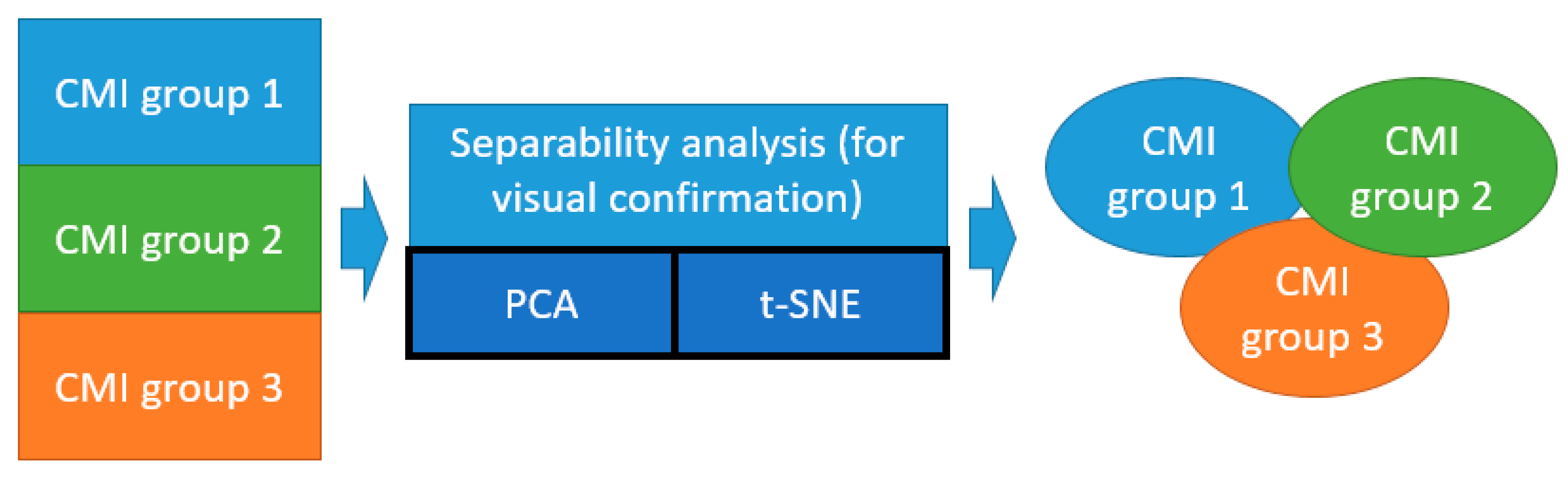
An illustration of the idea of our study is shown in Figure 1a. A list of corresponding ML models is given in Figure 1b. Models 1–3 were used to verify the homogeneity of the CMI groups, and Model 4 was used to test the separation between the TBI and GBM groups.
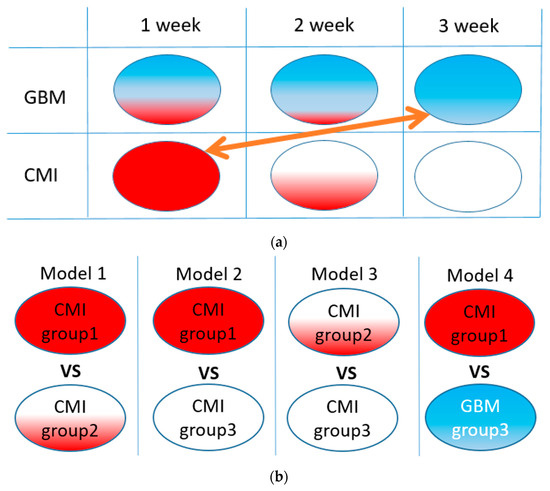
Figure 1.
The idea of the study (a): red area illustrates the CMI state, blue, the GBM state, and white area, the healthy state. Arrow means comparison of groups for TBI and GBM differentiation. List of ML binary models under study (b).
Contrary to our previous work, the homogeneity of the CMI groups was tested by the unsupervised ML methods to prove that effect of CMI is detectable by THz spectroscopy. Both pre-processing and ML hyperparameters were optimized to achieve robust models. The effects of PCA and t-SNE parameters on an exploratory analysis of the THz data were revealed. Finally, the informative THz sub-bands allowing for distinguishing the CMI and GBM groups were selected.
This paper is structured as follows: Section 1 describes the known methods for GBM diagnostics, indicates the role of traumatic brain injury in GBM development, describes preliminary studies, sets the research problem, and provides an experimental design. Section 2 contains a description of the experiment, the characteristics of the animals, a description of the THz spectrometer, and the measurement techniques. These were the ML methods used below. Some additional information for this section is in the Supplementary Materials (Section S1. Experiment, Tables S1 and S2). Section 3 describes the results of the study. Some of the results are presented in the Supplementary Materials (Figures S1–S4). The discussion and concluding remarks are in Section 4 and Section 5, accordingly.
2. Materials and Methods
2.1. Samples
The study was carried out using specific-pathogen-free male SCID mice aged 6–7 weeks. The Inter-institutional Commission on Biological Ethics of the Institute of Cytology and Genetics, Siberian Branch of the Russian Academy of Sciences granted permission for the study (Permission #78, 16 April 2021) in accordance with EU Directive 2010/63/EU and the ARRIVE 2.0 recommendations. The mice were maintained under controlled conditions, namely, temperature, 22–26 °C; relative humidity, 30–50%; and 12/12 light/dark periods with dawn at 02:00 [61,64]. A model of experimental glioblastoma was implemented, in which a cell suspension (500,000 U87 MG cells per animal) in the culture medium (DMEM\F-12, Thermo Fisher Scientific, Waltham, MA, USA) with a 5 µL volume was introduced into the subcortical brain structure through a hole in the animal’s cranium [61,64]. These mice are referred to as the GBM groups. The mice corresponding to the CMI groups were injected in a similar manner with 5 µL of the culture medium. Intravital MRS was performed on the anesthetized animals before surgery and on days 7, 14, and 21 after the injection [64]. The tumor size measurements and neuro-metabolites analysis were performed using a horizontal 11.7 Tesla MRI tomograph (Biospec 117/16; Bruker, Billerica, MA, USA) [58,61,64]. Additional details about the experimental design are presented in the Supplementary Materials.
On the 7th, 14th, and 21st days after the injection, the mice were decapitated, blood samples were collected, and then centrifuged for 15 min at 1000× g. Next, the serum was placed in individual tubes and frozen at −80 °C. Before spectral measurements, the serum samples were defrosted. The numbers of collected serum samples in each group are presented in Table 2.
Table 2.
Numbers of blood serum samples in each group *.
2.2. THz Spectroscopy
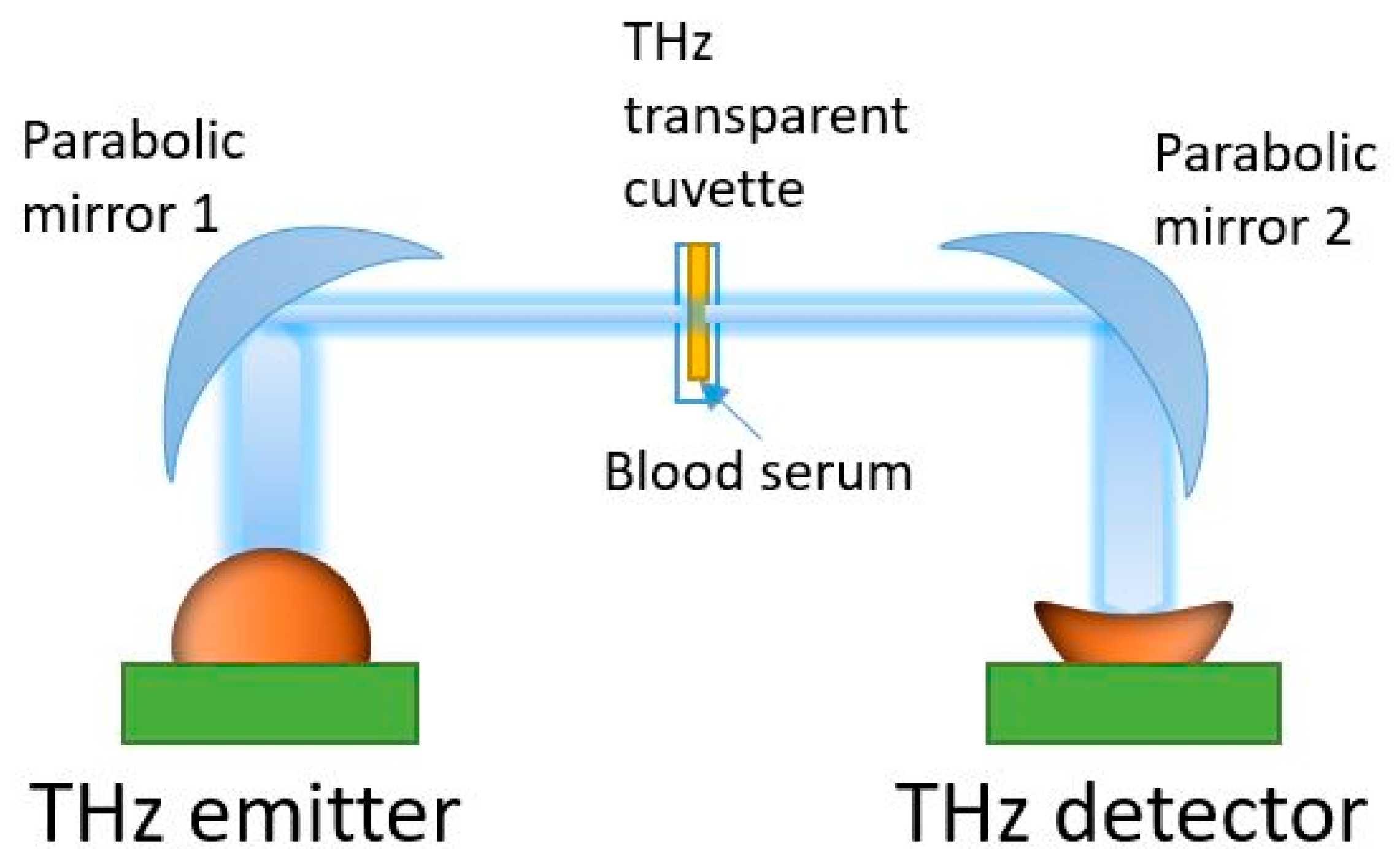
Spectral measurements were performed in the 0.3–1.7 THz range using a THz TDS spectrometer T-SPEC (EKSPLA, Vilnius, Lithuania). This has a spectral resolution of 10 GHz, two delay lines, fast and slow, to provide real-time data acquisition with a 10 spectra/s speed, and a dynamic range of >90 dB at 0.4 THz [22,58]. All measurements were carried out at a temperature of 21 ± 1 °C. Specially designed disposable cuvettes were produced from Watson material (Bestfilament, Tomsk, Russia) using a Designer X PRO 3D printer (PICASO 3D, Moscow, Russia) [58,66]. This material has an acceptable transparency in the THz spectral range [67]. The thickness of the cuvette internal cavity was 0.5 mm. In the THz-TDS spectrometer, the THz wave was focused onto the cuvette center using parabolic mirrors (see Figure 2). A reference signal was recorded with an empty cuvette. Then, without changing the position, the cuvette was filled with a serum sample (50 µL volume) using an automatic dispenser. An individual cuvette and dispenser tip were used for each sample analysis. The THz spectra measurement of a sample was conducted in six spatial points evenly distributed on the cuvette surface within a mesh grid were selected, with 0.1 mm steps in the horizontal and vertical directions. Averaging over 256 spectra was performed for each point of the 2D scans to reduce noise. The conversion of the signal from the time domain to the frequency domain was carried out using the Terravil TRS-16 software version 1.1.2.6 (TeraVil Ltd., Vilnius, Lithuania).

Figure 2.
THz time-domain spectrometer used in the transmission mode.
In a transmission scheme, the THz spectrometer measures the complex transmission coefficient of a sample: where is the complex electric field strength of the THz wave transmitted through the cuvette with a liquid sample, is the complex electric field strength of the THz wave transmitted through the empty cell, and is the frequency of the THz wave (see Figure 2). There is a quantitative relationship between the measured complex transmission coefficient of a substance and its dielectric characteristics [34,35,36]. When the reference signal of different samples has a low dispersion, it makes sense to consider only the intensity of the signal on the output of the THz wave detector. This approach has been proven to work well in conjunction with machine learning methods [22,58].
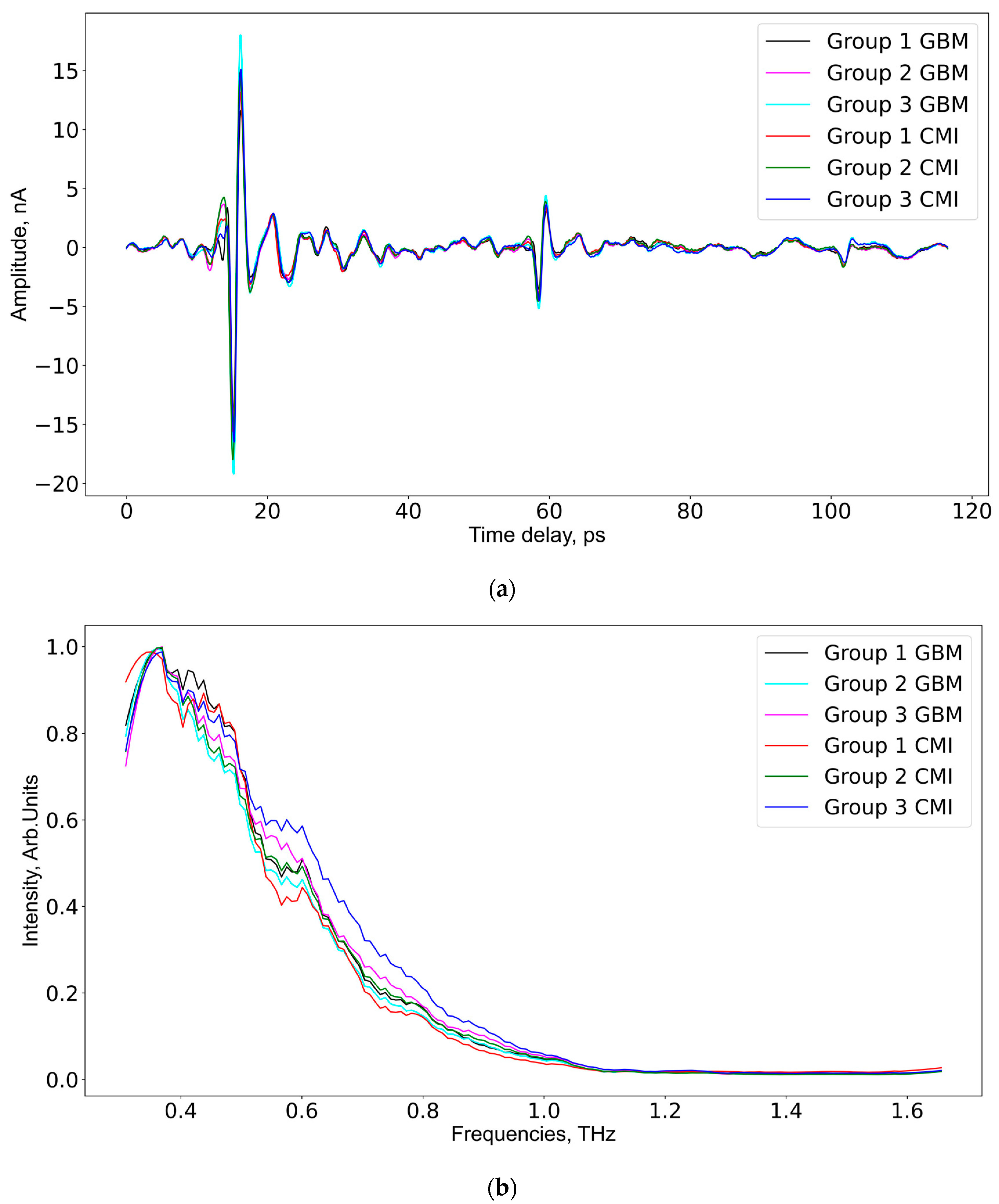
As aforementioned, each serum sample was measured at six different spatial points 256 times, so 1536 THz spectra per sample were measured. After averaging at a spatial point, only 6 spectra remained. In total, according to the number of serum samples in each group (see Table 2), the data for GBM group 1 and CMI group 1 consisted of 30 spectra for every group; the data for GBM group 2 and CMI group 2 consisted of 60 spectra for every group; the data for GBM group 3 included 42 spectra; and the data for CMI group 3 included 60 spectra. The frequency domain mean intensity signal values and time domain spectra of the samples from the GBM and CMI groups are presented in Figure 3. The mean spectrum for the samples from the CMI group 1 has lower intensities compared to similar spectra from CMI groups 2 and 3.
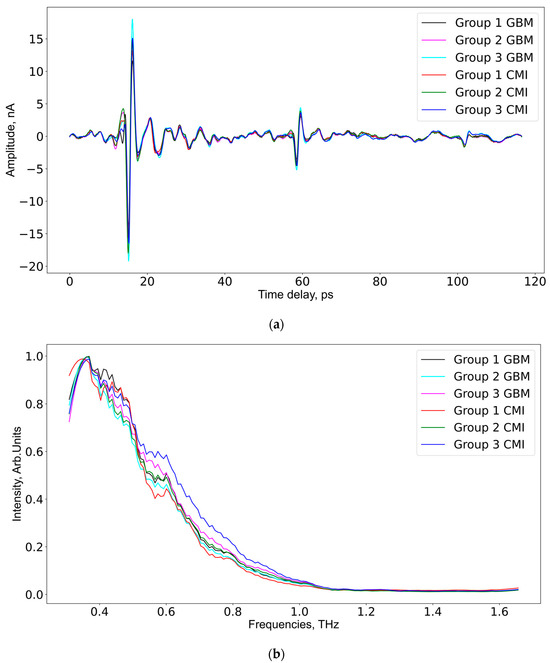
Figure 3.
The averaged THz spectra in the time domain (a) and the frequency domain (b) for all studied groups.
2.3. Machine Learning Methods
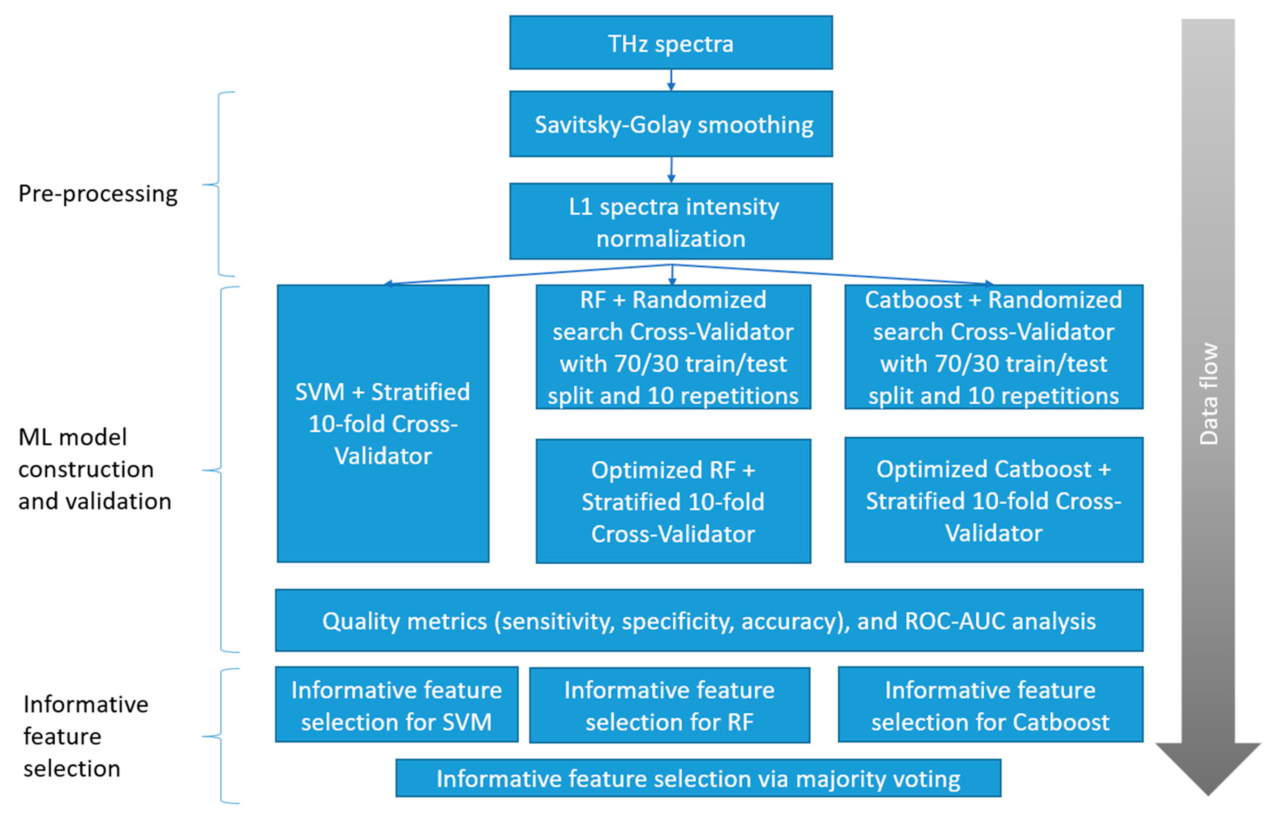
Two dimensionality reduction algorithms (PCA and t-SNE) and three classification algorithms (SVM, RF, and Catboost implementation of XGBoost) were applied to the THz spectral data. PCA (sklearn.decomposition.PCA) was applied along with t-SNE (sklearn.manifold.TSNE), without standard scaling. The proposed ML pipeline (Figure 4) includes the following steps: pre-processing; ML model construction and validation; and informative feature selection. The ML model construction and validation used the same algorithms, but different optimized parameters. The optimal values for each pair of groups are calculated based on accuracy metrics and given in Table S2, Supplementary Materials.
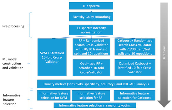
Figure 4.
Proposed ML pipeline steps.
During the pre-processing, each THz spectrum was smoothed by the Savitsky–Golay filter [68]. The impact of the filter parameters (filtering window width—window_size, and degree of polynomial smoothing—polyoder) on the classifier performance was estimated by the cross-validation procedure. The parameter names are given according to the library scipy.signal.savgol_filter in Python. Next, the THz data were normalized by the maximum intensity value (vector normalization) for an appropriate spectra comparison. The effect of data centralization (statistical procedure of subtracting mean and dividing by variance) on the dimensionality reduction methods was tested.
The unsupervised ML methods (PCA and t-SNE) were used to verify the homogeneity of the CMI groups (Figure 5).
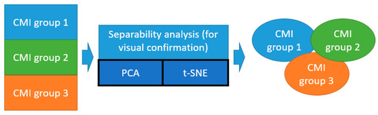
Figure 5.
Illustration of application of unsupervised ML methods (t-SNE and PCA) for the separability analysis of the CMI groups.
The number of principal components (PC) for PCA was limited to ten, with the highest explained variance for the visual comparison. The optimized t-SNE parameters were perplexity (15) and number of iterations (300). The latter did not have any impact on the separability of the data. The perplexity significantly changes the distribution of points after projection, so the choice of an appropriate value was crucial.
Catboost was chosen because of its excellent computational performance. The optimal values of the hyperparameters for the RF and Catboost ML models were estimated by the RandomizedSearchCV algorithm from the sklearn.model.selection library. Using cross-validation on a user-defined parameter search grid, the algorithm determined the prediction data model with the highest performance metrics for a definite ML algorithm. The choice of hyperparameters for optimization usually depends on human expertise. A dense parameter grid will lead to unreasonable computational costs, and even evolutionary optimization algorithms will require a huge amount of processing time. Randomized search is used to speed up the process. This step was performed to avoid instability of the feature selection algorithms on the models with default parameters.
The linear kernel SVM performance can be optimized by a regularization parameter (C). A lower C avoids overfitting, and a higher C allows the fine-tuning of the data model. Usually, SVMs are used with default parameters. In RF implementation, the following parameters of the search grid were used: number of trees in the random forest (50, 100, and 1000), maximum number of levels in each tree (from 10 to 120 with step 12), minimum sample number to split a node (2, 6, and 10), minimum sample number that can be stored in a leaf node (1, 3, and 4), and using bootstrap for data points sampling. The number of cross-validation runs (RandomizedSearchCV) was set to 10. The Catboost parameters grid: learning rate (0.03, 0.1), depth (2, 4, 6, 10), and l2_leaf_reg (1, 3, 5, 7, 9) were optimized by the build-in catboost.randomized_search procedure. A complete list of the optimized values of these parameters is shown in Table S2, Supplementary Materials.
The efficiency of the ML models was estimated using 10-fold cross validation in terms of the sensitivity, specificity, accuracy, and ROC-AUC values. Confidence matrices of each fold were summarized, and final performance metrics were computed. Informative feature selection was performed by the built-in procedures.
3. Results
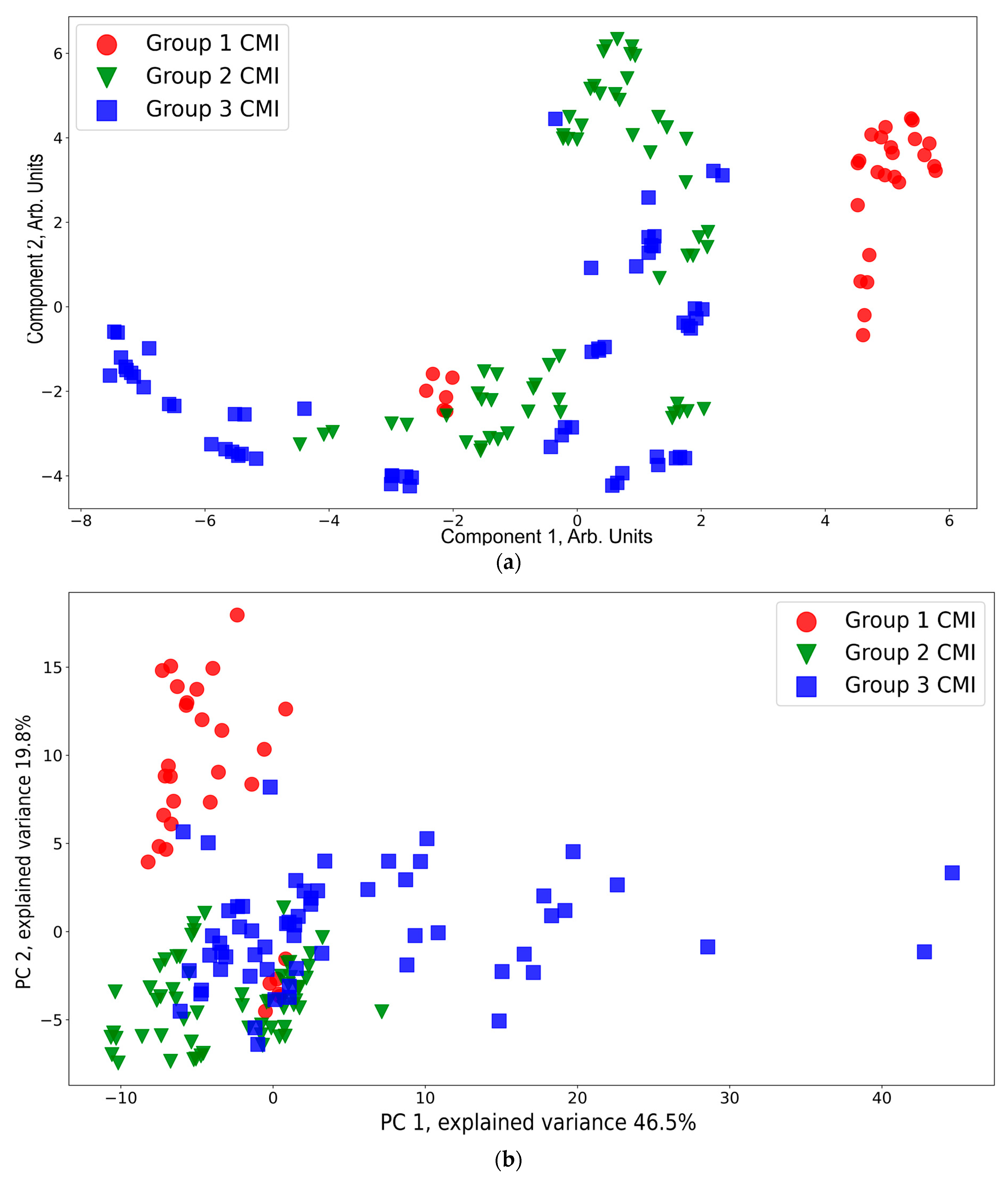
A presentation of the CMI groups in a feature space using t-SNE and PCA is shown in Figure 6. According to the t-SNE data presentation (Figure 6a), CMI group 1 (except six red dots near the region with coordinates (−2, −2) corresponding to the spectra of one sample) is separated from CMI groups 2 and 3. The points from CMI groups 2 and 3 are widely spread and mixed between each other. This is owing to the side effects of the injections still being in place. This result is consistent with the conclusions based on a 1H-MRS analysis that neuro inflammation disappears by the third week [64]. According to the PCA data presentation (Figure 6b), the CMI groups separation is worse compared to that of t-SNE. Additional PCA projections for the CMI groups are shown Figure S1, Supplementary Materials, which confirms that there is no separability between the groups for the additional principal component projections.

Figure 6.
t-SNE (a) and PCA (b) visualization of the CMI groups.
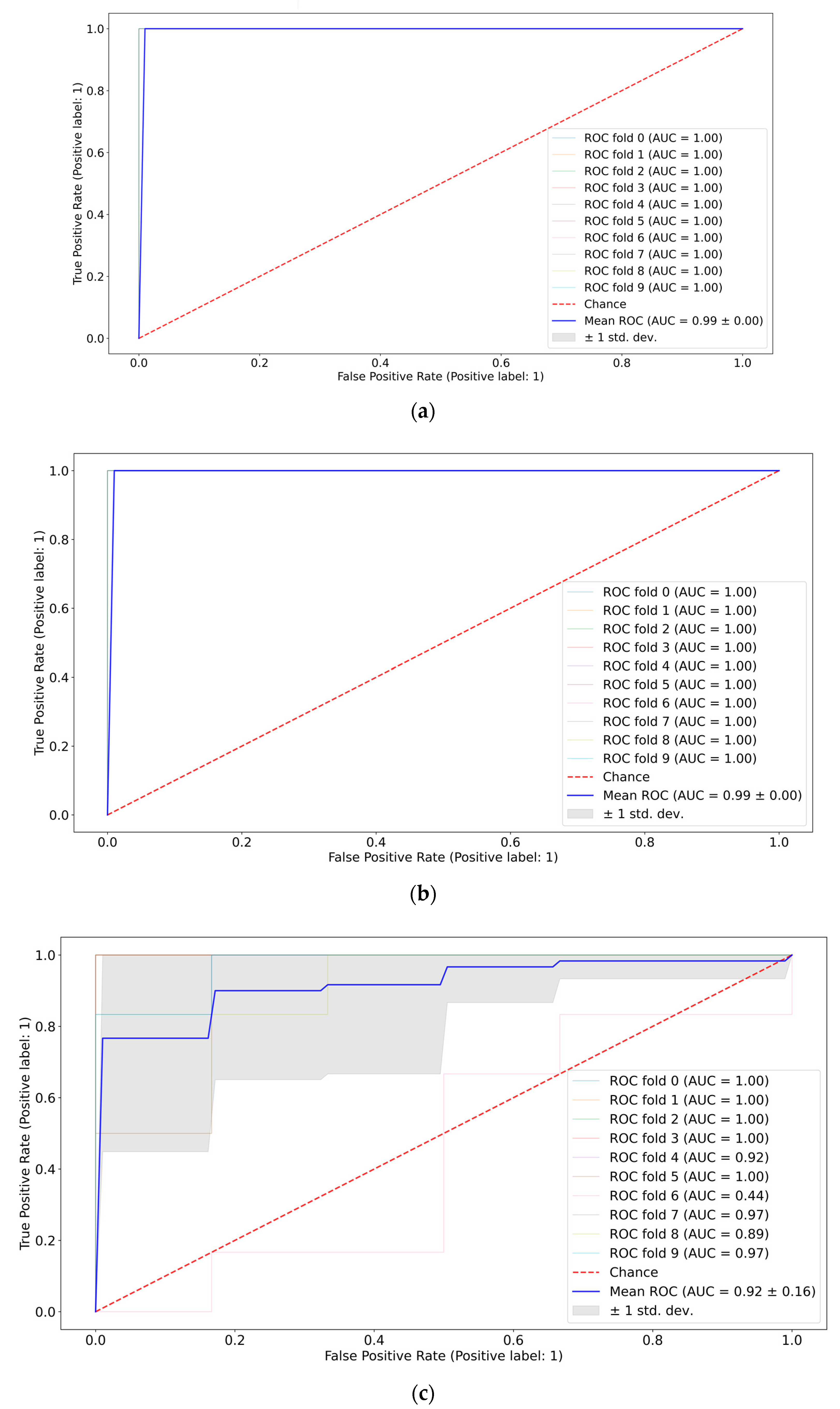
A pair-wise comparison of the CMI groups (the first vs. the second weeks, the first vs. the third weeks, and the second vs. the third weeks) in terms of quality metrics and informative features was conducted. The best ROC-AUC metrics were achieved by the SVM and Catboost classifiers (see Figure 7). Full ROC-AUC graphs for all classifiers and all CMI groups are presented in Figure S2, Supplementary Materials. All classifiers demonstrated very good performance metrics (see Table 3). The ideal separability was between CMI groups 1 and 3, which confirms previous conclusions about the neuro inflammation period. CMI groups 2 and 3 are not distinguished very accurately (see Figure S2d,f), so the extraction of informative features differentiating them can be misleading.
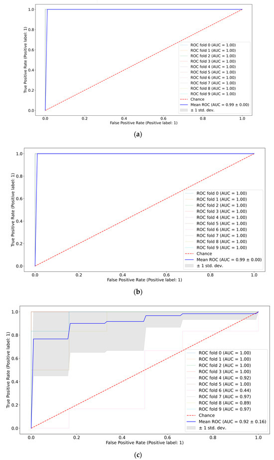
Figure 7.
ROC-AUC analysis of CMI groups: 1st vs. 2nd weeks using SVM (a), 1st vs. 3rd weeks using Catboost (b), and 2nd vs. 3rd weeks using Catboost (c).
Table 3.
Mean ROC-AUC metrics of the CMI groups for different classifiers.
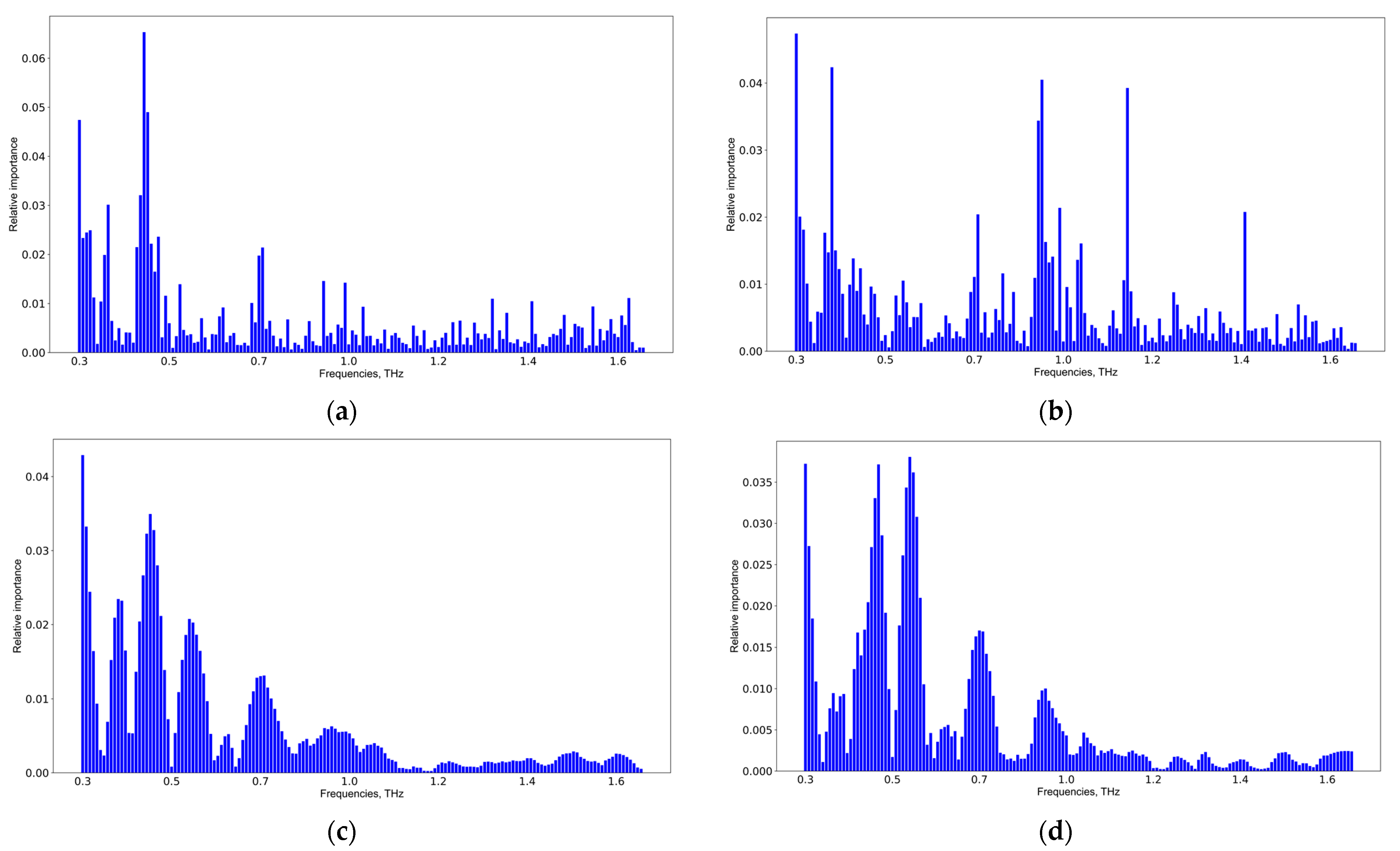
The results of the informative feature extraction by Catboost and SVM allowing the pair-wise classification of CMI group 1 versus CMI group 2 and CMI group 1 versus CMI group 3 are shown in Figure 8. A detailed analysis of the informative features for all groups and classifiers is presented in Figure S3, Supplementary Materials. The results of the SVM application coincide, but those of the Catboost application are different. The latter is explained due to the computation of informative features in the extreme gradient boosting methods. The more weight a feature has, the more often it is used to separate data in each tree. Thus, a simple voting scheme was used for verifying the informative features discovered by different classifiers, and the following spectral features: 0.35, 0.45, 0.55, 0.7, 0.9, and 1.05 THz were selected. These frequencies are potential TBI markers.

Figure 8.
Informative feature analysis of CMI groups: 1st vs. 2nd weeks using Catboost (a), 1st vs. 3rd weeks using Catboost (b), 1st vs. 2nd weeks using SVM (c), and 1st vs. 3rd weeks using SVM (d).
CMI group 1 and the GBM group 3 were compared to differentiate TBI and GBM (see Table 4). All classifiers are equally good in terms of AUC metrics, however, the specificity value for SVM and RF has a high variance.
Table 4.
Mean and variance of AUC, sensitivity, specificity, and accuracy metrics of the TBI and the GBM groups’ differentiation by various classifiers.
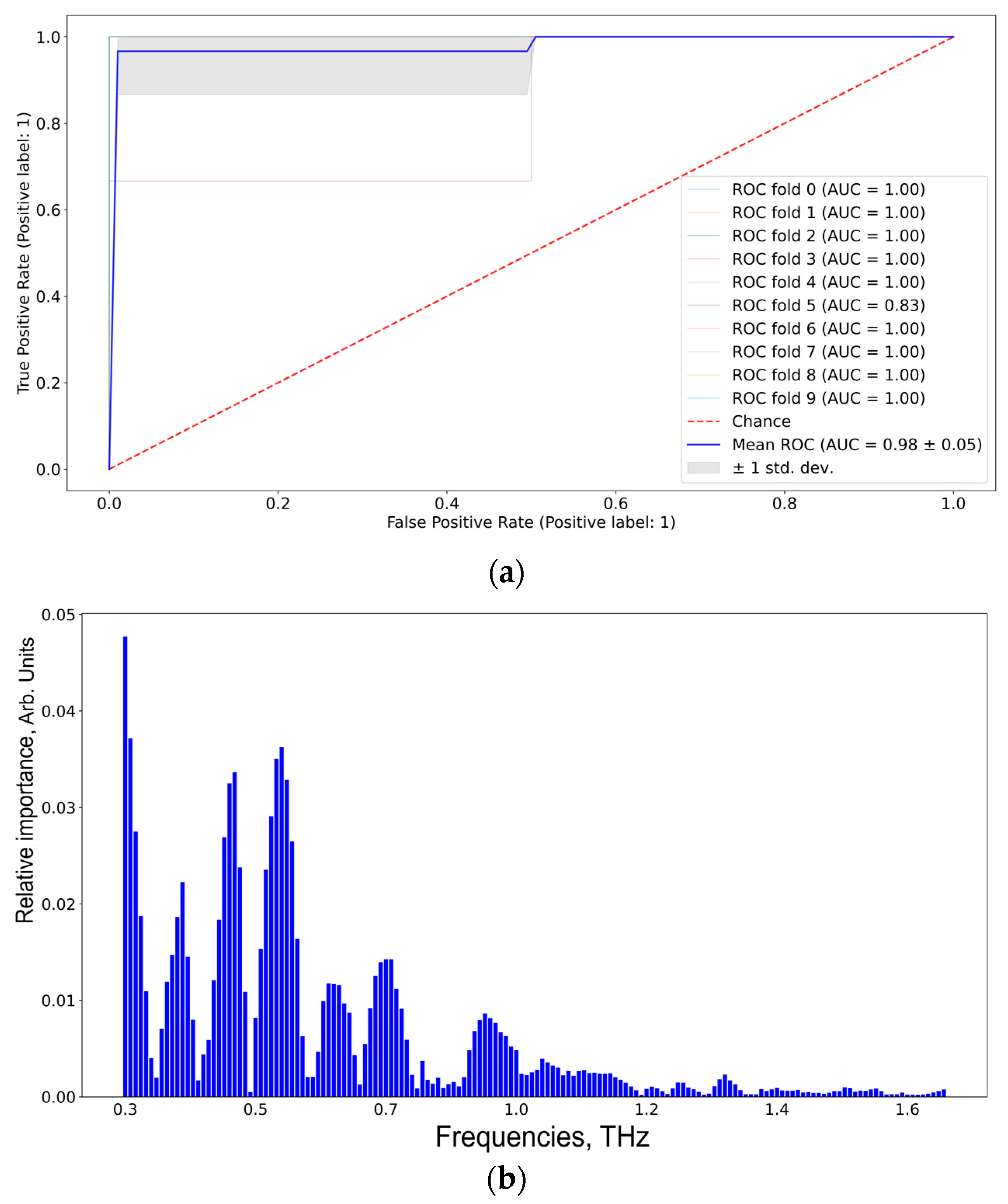
According to Figure 9, the informative features distinguishing TBI and GBM via SVM are 0.37, 0.40, 0.55, 0.60, 0.70, and 0.90 THz. The results were the same for RF and Catboost (see Figure S4, Supplementary Materials).

Figure 9.
ROC-AUC analysis of SVM classifier (a) of the TBI group vs. the GBM group and the corresponding informative features (b).
4. Discussion
To study glioblastoma development and find adequate therapeutic approaches, various experimental models of glioblastoma have been developed [60,69]. In the most popular models, tumor cells are injected into the brain of an animal [61]. However, the injection procedure is itself a factor of TBI [63,64,70]. A needle insertion into brain structures and the injection of different substances lead to the development of neuro inflammation within the first 24 h after such manipulations [63,70,71]. MRS in vivo measurements showed decreases in tNAA (the sum of N-acetylaspartate and N-acetylaspartylglutamic acid) and tCho (the sum of glycerophosphocholine and phosphocholine) levels on the 7th day after CMI [64], indicating possible neuronal death and axonal damage associated with TBI [72]. The level of gamma aminobutyric acid also decreased, which is consistent with the dynamics of the level of this metabolite after TBI [73].
The major goal of this work was to discover the informative features in blood serum THz spectra, which differentiate TBI and glioblastoma. It should be noted that the blood serum samples analyzed here were from the same mice, which were analyzed in vivo by MRS (these data were presented in Ref. [64]). According to the presented results, the mean THz spectrum of the blood serum samples from CMI group 1 (day 7 after the injection) had lower intensities compared to similar spectra of CMI groups 2 and 3 (see Figure 3b). The results of the PCA and t-SNE processing of the CMI groups’ THz spectra showed that CMI group 1 was separated from CMI groups 2 and 3 (see Figure 6). This is consistent with the data regarding the temporal development of TBI [63,64,70,71]. Therefore, CMI group 1 was concluded to correspond to the TBI state.
The development of neuro inflammation after CMI has a limited temporal period. After day 14 of the experiment, the histological analysis did not demonstrate a significant difference in the brains after CMI and healthy brains [70]. The aforementioned neuro metabolites’ return to the levels of healthy mice was observed by day 21 after the CMI, which confirms the restoration of neurons and their viability [64]. Therefore, CMI group 3 can be used as a group of animals that no longer show clear signs of neuro inflammation and TBI. The mice in this group can be considered conditionally healthy. This was also confirmed by the fact that the mean THz intensity of CMI group 3 was higher compared to that of CMI groups 1 and 2 (see Figure 3b), growing closer to the amplitude of the THz spectrum of water [58]. As mentioned above, changes in the relative proportions of free and bound water and in relaxation times for either of these states can all be observed by THz spectroscopy [34,46,65]. Changes in blood composition at diabetes mellitus [74], liver cancer [75], and thyroid cancer [38], as well as GBM [65], were shown by us to be detected in the blood THz absorption spectra.
The development of neuro inflammation [63,64,71] in experimental models of glioblastoma [61,64] and the subsequent development of the tumor lead to the release of inflammatory and oncological molecular markers into the blood [14]. Molecular markers’ discovery using THz spectroscopy is a complex and currently unsolved problem. ML methods allow for building predictive data models and finding informative frequencies in the THz spectral range associated with similar molecular markers [76,77,78].
A THz spectra analysis of blood serum from the CMI and GBM groups of mice to estimate the THz spectral regions responsible for the differentiation of glioblastoma from TBI was conducted. Two dimensionality reduction algorithms (PCA and t-SNE) were used for data visualization. Three supervised machine learning algorithms—SVM, RF, and Catboost—were used for classification and informative feature selection. The verification of the data models’ efficiency was performed by 10-fold cross-validation. All algorithms were implemented in Python 3.9 and scikit-learn library.
To obtain robust results, data standardization for PCA (mean value subtracting and dividing by standard deviation) was used. This step is useful if the data have a high level of variability, which is the case for THz spectra. Unlike PCA, the t-SNE algorithm considers the distances between data points in the original space, and it delivered better results without standardization. Euclidian and cosine distances for t-SNE were compared. The latter showed a better separability.
The suggested ML pipeline allowed for selecting informative THz frequencies to differentiate CMI group 1 from CMI group 3 (see Figure 7). The informative features were 0.35, 0.45, 0.55, 0.7, 0.9, and 1.05 THz. These groups had an excellent separability, and the AUC was 0.99 for all classifiers (see Figure 6 and Table 3), which also confirms the correctness of the definition of CMI group 1 (day 7 after culture medium injection) as TBI. In Ref. [79], rat blood serum at different stages of experimental blast-induced traumatic brain injury (bTBI) was studied in the attenuated total reflection (ATR) mode by THz-TDS and ML methods. This study was carried out within 24 h after the experimental trauma. The THz absorption spectra were analyzed by combining PCA and two machine learning algorithms (k-Nearest neighbor and SVM) to identify the degree of bTBI. The SVM classifier provided the best results on the test set with the highest diagnostic accuracy of 95.5%. The authors concluded that ATR THz-TDS and ML have great potential for the early diagnosis of bTBI. However, the authors did not select informative THz frequencies to separate groups.
The results of the pair-wise comparison of CMI group 1 and GBM group 3 to differentiate between TBI and glioblastoma are shown in Table 4 and Figure 8. The same frequencies obtained for SVM, RF, and Catboost, coupled with high performance metrics, imply the robustness of the used ML algorithms. The proposed ML pipeline allowed us to differentiate the TBI and GB groups with 95% sensitivity, 100% specificity, and 97% accuracy. The informative features for distinguishing TBI and GBM were 0.37, 0.40, 0.55, 0.60, 0.70, and 0.90 THz.
A common strategy for the verification of feature selection procedures is the removal of these frequencies and then the calculation of performance metrics. This approach is good for non-correlating features, yet for the case of THz spectra, it is not so effective. To verify their importance, frequencies with the highest importance values but also a surrounding one should be removed. The experimental results showed a drop in the average sensitivity, specificity, accuracy, and precision of up to 13% for SVM, up to 7% for RF, and up to 17% for Catboost. This proved that the selected frequencies were indeed informative for the task under study.
In our previous study of mouse blood serum and the dynamics of U87 glioblastoma development using THz-TDS [58], the ML pipeline included THz spectra smoothing using the Savitsky–Golay filter, outlier removal using the isolated forest method, the subtraction of the mean and normalizing data to the standard deviation, informative feature extraction, and dimensionality reduction by PCA. The predictive data model was created using linear SVM. By comparing GBM group 3 (the 21st day after U87 cell injection) and the corresponding control group 3 (the 21st day after culture medium injection), the following informative THz frequencies differentiating these groups were selected: 0.22, 0.56, 1.0, 1.2, 1.48, and 1.52 THz. As can be seen, these informative frequencies did not overlap with those selected in this study. A possible reason for this was that TBI and GBM were compared here, contrary to the GBM versus healthy groups study in the previous work. We cannot accurately indicate specific metabolites, because the molecules’ absorption bands overlapped in the THz spectral range. Moreover, there are more than 4600 metabolites currently known in human blood serum [80], and the interactions between them are yet to be fully established.
5. Conclusions
In this work, the popular glioblastoma model based on glioblastoma cells’ injection into the mouse brain was used. But the injection itself can be considered as a TBI, and it is necessary to differentiate metabolic disorders in the mouse brain caused by traumatic brain injuries or/and glioblastoma development. Mouse blood serum was analyzed by THz spectroscopy. In the first step, the homogeneity of the experimental groups with a cultural medium injection was tested by unsupervised ML methods to prove that CMI group 1 (day 7 after CMI) was associated with a TBI state. In the second stage, this group was compared with the group with the largest volume of glioblastoma (day 21 after injection of glioblastoma cells) to differentiate between glioblastoma and TBI. The constructed prediction data models were verified by the 10-fold cross-validation technique coupled with an ROC-AUC analysis to ensure the repeatability of the results. Finally, informative THz bands were selected, which had the most impact on the separability between the glioblastoma group and the TBI group. As far as we know, this is the first work in which differences in the blood serum THz spectra from small animals with glioblastoma and TBI were studied. The presented results can be further expanded to the study of patient blood and appropriate diagnostic method development.
Data quality strongly affects the prediction data model efficiency. The robustness of these models can be increased by optimizing the hyperparameters. Considering a combination of such parameters for each method in the ML pipeline leads to high computational costs. Understanding what effect each parameter has becomes crucial.
The limitations of the presented work are the following. ML models require plenty of marked data to construct a reliable prediction data model, but glioma models are subjected to a high variance due to the complex physiology of the carcinogenic process in glia. Only “white box” algorithms were tested, yet complex “black box” models coupled with the SHAP technique may produce better results. Still, the latter is more computationally intensive. THz spectroscopy of biofluids is difficult because of strong water absorption, so preliminary drying/lyophilization of samples is preferable. The binary classifier performance metrics can also be enriched by the use of Matthews correlation coefficient, which is argued to be the next gold standard in the evaluation of supervised ML models.
Future work will be related to the data fusion of different modalities to increase diagnostic potential and reveal the metabolites of glioma in the blood. This metabolic profile can be discovered by Raman spectroscopy or MRS. Another option for improvements in ML models is a combination of THz and MRI/PET/CT imaging to visualize tumor boundaries that are crucial for surgery [81] and differentiate glioblastoma and TBI. Both intraoperative MRI and PET are extremely expensive and time-consuming. PET has a low resolution compared to THz and MRI [82]. The application of computer vision techniques based on convolutional neural networks significantly boosts the segmentation quality of MRI brain scans [83,84,85]. A combination of diagnostic MRI enhanced by ML methods and intraoperative THz visualizations could be a promising solution for glioma surgery.
Supplementary Materials
The following supporting information can be downloaded at: https://www.mdpi.com/article/10.3390/app14072872/s1, Experiment; Figure S1: Additional PCA projections of the CMI groups. PCA score plot for PC 3 and PC 4 (a); PC 5 and PC 6 (b); PC 7 and PC 8 (c); PC 9 and PC 10 (d); Figure S2: ROC-AUC analysis for: the CMI group 1 vs. the CMI group 2, SVM method (a); the CMI group 1 vs. the CMI group 2, RF method (b); the CMI group 1 vs. the CMI group 2, Catboost method (c); the CMI group 2 vs. the CMI group 3, SVM method (d); the CMI group 2 vs. the CMI group 3, RF method (e); the CMI group 2 vs. the CMI group 3, Catboost method (f); the CMI group 1 vs. the CMI group 3, SVM method (g); the CMI group 1 vs. the CMI group 3, the CMI RF method (h); the CMI group 1 vs. the CMI group 3, Catboost method (i); Figure S3: Informative features for: the CMI group 1 vs. the CMI group 2, SVM method (a); the CMI group 1 vs. the CMI group 2, RF method (b); the CMI group 1 vs. the CMI group 2, Catboost method (c); the CMI group 2 vs. the CMI group 3, SVM method (d); the CMI group 2 vs. the CMI group 3, RF method (e); the CMI group 2 vs. the CMI group 3, Catboost method (f); the CMI group 1 vs. the CMI group 3, SVM method (g); the CMI group 1 vs. the CMI group 3, CMI RF method (h); the CMI group 1 vs. the CMI group 3, Catboost method (i); Figure S4: the CMI group 1 vs. the GBM group 3: SVM method ROC-AUC analysis (a), informative features (b); RF method ROC-AUC analysis (c), informative features (d); Catboost method ROC-AUC analysis (e), informative features (f); Table S1. Formulas for model performance evaluation metrics; Table S2. Optimized parameters’ values for ML pipeline. References [86,87] are cited in the Supplementary Materials.
Author Contributions
Conceptualization, D.A.V., O.P.C., Y.V.K. and N.A.N.; methodology, O.P.C., A.G.P., Y.V.K. and N.A.N.; software, D.A.V., D.A.O. and A.G.P.; formal analysis, D.A.O., D.A.V., A.G.P. and T.V.K.; data curation, T.V.K.; writing—original draft preparation, D.A.V., O.P.C., T.V.K. and D.A.O.; writing—review and editing, D.A.V., D.A.O., A.G.P., T.V.K., Y.V.K., O.P.C. and N.A.N.; supervision, Y.V.K.; funding acquisition, N.A.N. All authors have read and agreed to the published version of the manuscript.
Funding
The work was carried out within the framework of the State assignment project of the IA&E SB RAS # FWNG-2024-0025. The work of O.P.C. was partially supported within the state assignment of NRC “Kurchatov Institute”. The work of Y.V.K. was supported by the Tomsk State University Development Programme (Priority-2030).
Institutional Review Board Statement
The study was conducted according to the guidelines of the Declaration of Helsinki, and approved by the Inter-Institutional Commission on Biological Ethics at the Institute of Cytology and Genetics, Siberian Branch of the Russian Academy of Sciences (Permission #78, 16 April 2021).
Informed Consent Statement
Not applicable.
Data Availability Statement
The raw data supporting the conclusions of this article will be made available by the authors on request.
Conflicts of Interest
The authors declare no conflicts of interest. The funders had no role in the design of the study; in the collection, analysis, or interpretation of data; in the writing of the manuscript, or in the decision to publish the results.
References
- Hishii, M.; Matsumoto, T.; Arai, H. Diagnosis and Treatment of Early-Stage Glioblastoma. Asian J. Neurosurg. 2019, 14, 589–592. [Google Scholar] [CrossRef] [PubMed]
- Ostrom, Q.T.; Cioffi, G.; Waite, K.; Kruchko, C.; Barnholtz-Sloan, J.S. CBTRUS Statistical Report: Primary Brain and Other Central Nervous System Tumors Diagnosed in the United States in 2014–2018. Neuro-Oncology 2021, 23 (Suppl. S3), iii1–iii105. [Google Scholar] [CrossRef] [PubMed]
- Tykocki, T.; Eltayeb, M. Ten-year survival in glioblastoma. A systematic review. J. Clin. Neurosci. 2018, 54, 7–13. [Google Scholar] [CrossRef] [PubMed]
- Komori, T. The 2021 WHO classification of tumors, 5th edition, central nervous system tumors: The 10 basic principles. Brain Tumor Pathol. 2022, 39, 47–50. [Google Scholar] [CrossRef] [PubMed]
- Auer, T.A. Advanced MR techniques in glioblastoma imaging—Upcoming challenges and how to face them. Eur. Radiol. 2021, 31, 6652–6654. [Google Scholar] [CrossRef]
- Bernstock, J.D.; Gary, S.E.; Klinger, N.; Valdes, P.A.; Ibn Essayed, W.; Olsen, H.E.; Chagoya, G.; Elsayed, G.; Yamashita, D.; Schuss, P.; et al. Standard clinical approaches and emerging modalities for glioblastoma imaging. Neuro-Oncol. Adv. 2022, 4, vdac080. [Google Scholar] [CrossRef] [PubMed]
- Mărginean, L.; Ștefan, P.A.; Lebovici, A.; Opincariu, I.; Csutak, C.; Lupean, R.A.; Coroian, P.A.; Suciu, B.A. CT in the Differentiation of Gliomas from Brain Metastases: The Radiomics Analysis of the Peritumoral Zone. Brain Sci. 2022, 12, 109. [Google Scholar] [CrossRef]
- Swanson, K.R.; Chakraborty, G.; Wang, C.H.; Rockne, R.; Harpold, H.L.P.; Muzi, M.; Adamsen, T.C.H.; Krohn, K.A.; Spence, A.M. Complementary but distinct roles for MRI and 18F-Fluoromisonidazole PET in the assessment of human glioblastomas. J. Nucl. Med. 2009, 50, 36–44. [Google Scholar] [CrossRef] [PubMed]
- Schultz, S.; Pinsky, G.S.; Wu, N.C.; Chamberlain, M.C.; Rodrigo, A.S.; Martin, S.E. Fine needle aspiration diagnosis of extracranial glioblastoma multiforme: Case report and review of the literature. CytoJournal 2005, 2, 19. [Google Scholar] [CrossRef]
- Katzendobler, S.; Do, A.; Weller, J.; Dorostkar, M.M.; Albert, N.L.; Forbrig, R.; Niyazi, M.; Egensperger, R.; Thon, N.; Tonn, J.C.; et al. Diagnostic Yield and Complication Rate of Stereotactic Biopsies in Precision Medicine of Gliomas. Front. Neurol. 2022, 13, 822362. [Google Scholar] [CrossRef]
- Lan, Y.L.; Zhu, Y.; Chen, G.; Zhang, J. The Promoting Effect of Traumatic Brain Injury on the Incidence and Progression of Glioma: A Review of Clinical and Experimental Research. J. Inflamm. Res. 2021, 14, 3707–3720. [Google Scholar] [CrossRef] [PubMed]
- Lone, S.N.; Nisar, S.; Masoodi, T.; Singh, M.; Rizwan, A.; Hashem, S.; El-Rifai, W.; Bedognetti, D.; Batra, S.K.; Haris, M.; et al. Liquid biopsy: A step closer to transform diagnosis, prognosis and future of cancer treatments. Mol. Cancer 2022, 21, 79. [Google Scholar] [CrossRef] [PubMed]
- Wang, L.; Liu, X.; Yang, Q. Application of Metabolomics in Cancer Research: As a Powerful Tool to Screen Biomarker for Diagnosis, Monitoring and Prognosis of Cancer. Biomark. J. 2018, 4, 12. [Google Scholar] [CrossRef]
- Ali, H.; Harting, R.; de Vries, R.; Ali, M.; Wurdinger, T.; Best, M.G. Blood-Based Biomarkers for Glioma in the Context of Gliomagenesis: A Systematic Review. Front. Oncol. 2021, 11, 665235. [Google Scholar] [CrossRef] [PubMed]
- Poinsignon, V.; Mercier, L.; Nakabayashi, K.; David, M.D.; Lalli, A.; Penard-Lacronique, V.; Quivoron, C.; Saada, V.; De Botton, S.; Broutin, S.; et al. Quantitation of isocitrate dehydrogenase (IDH)-induced D and L enantiomers of 2-hydroxyglutaric acid in biological fluids by a fully validated liquid tandem mass spectrometry method, suitable for clinical applications. J. Chromatogr. B 2016, 1022, 290–297. [Google Scholar] [CrossRef]
- Strain, S.K.; Groves, M.D.; Olino, K.L.; Emmett, M.R. Measurement of 2-hydroxyglutarate enantiomers in serum by chiral gas chromatography-tandem mass spectrometry and its application as a biomarker for IDH mutant gliomas. Clin. Mass Spectrom. 2020, 15, 16–24. [Google Scholar] [CrossRef]
- Miyauchi, E.; Furuta, T.; Ohtsuki, S.; Tachikawa, M.; Uchida, Y.; Sabit, H.; Obuchi, W.; Baba, T.; Watanabe, M.; Terasaki, T.; et al. Identification of blood biomarkers in glioblastoma by SWATH mass spectrometry and quantitative targeted absolute proteomics. PLoS ONE 2018, 13, e0193799. [Google Scholar] [CrossRef]
- Baranovičová, E.; Galanda, T.; Galanda, M.; Hatok, J.; Kolarovszki, B.; Richterová, R.; Račay, P. Metabolomic profiling of blood plasma in patients with primary brain tumours: Basal plasma metabolites correlated with tumour grade and plasma biomarker analysis predicts feasibility of the successful statistical discrimination from healthy subjects—A preliminary study. IUBMB Life 2019, 71, 1994–2002. [Google Scholar] [PubMed]
- Lee, J.E.; Jeun, S.S.; Kim, S.H.; Yoo, C.Y.; Baek, H.M.; Yang, S.H. Metabolic profiling of human gliomas assessed with NMR. J. Clin. Neurosci. 2019, 68, 275–280. [Google Scholar] [CrossRef]
- Godlewski, A.; Czajkowski, M.; Mojsak, P.; Pienkowski, T.; Gosk, W.; Lyson, T.; Mariak, Z.; Reszec, J.; Kondraciuk, M.; Kaminski, K.; et al. A comparison of different machine-learning techniques for the selection of a panel of metabolites allowing early detection of brain tumors. Sci. Rep. 2023, 13, 11044. [Google Scholar] [CrossRef]
- Cherkasova, O.; Peng, Y.; Konnikova, M.; Kistenev, Y.; Shi, C.; Vrazhnov, D.; Shevelev, O.; Zavjalov, E.; Kuznetsov, S.; Shkurinov, A. Diagnosis of Glioma Molecular Markers by Terahertz Technologies. Photonics 2021, 8, 22. [Google Scholar] [CrossRef]
- Cherkasova, O.; Vrazhnov, D.; Knyazkova, A.; Konnikova, M.; Stupak, E.; Glotov, V.; Stupak, V.; Nikolaev, N.; Paulish, A.; Peng, Y.; et al. Terahertz Time-Domain Spectroscopy of Glioma Patient Blood Plasma: Diagnosis and Treatment. Appl. Sci. 2023, 13, 5434. [Google Scholar] [CrossRef]
- Cameron, J.M.; Brennan, P.M.; Antoniou, G.; Butler, H.J.; Christie, L.; Conn, J.J.A.; Curran, T.; Gray, E.; Hegarty, M.G.; Jenkinson, M.D.; et al. Clinical validation of a spectroscopic liquid biopsy for earlier detection of brain cancer. Neurooncol. Adv. 2022, 4, vdac024. [Google Scholar] [CrossRef] [PubMed]
- Gray, E.; Cameron, J.M.; Butler, H.J.; Jenkinson, M.D.; Hegarty, M.G.; Palmer, D.S.; Brennan, P.M.; Baker, M.J. Early economic evaluation to guide the development of a spectroscopic liquid biopsy for the detection of brain cancer. Int. J. Technol. Assess Health Care 2021, 37, E41. [Google Scholar] [CrossRef] [PubMed]
- Cameron, J.M.; Butler, H.J.; Smith, B.R.; Hegarty, M.G.; Jenkinson, M.D.; Syed, K.; Brennan, P.M.; Ashton, K.; Dawson, T.; Palmer, D.S.; et al. Developing infrared spectroscopic detection for stratifying brain tumour patients: Glioblastoma multiforme vs. lymphoma. Analyst 2019, 144, 6736–6750. [Google Scholar] [CrossRef] [PubMed]
- Butler, H.J.; Brennan, P.M.; Cameron, J.M.; Finlayson, D.; Hegarty, M.G.; Jenkinson, M.D.; Palmer, D.S.; Smith, B.R.; Baker, M.J. Development of high-throughput ATR-FTIR technology for rapid triage of brain cancer. Nat. Commun. 2019, 10, 4501. [Google Scholar] [CrossRef] [PubMed]
- Theakstone, A.G.; Brennan, P.M.; Jenkinson, M.D.; Mills, S.J.; Syed, K.; Rinaldi, C.; Xu, Y.; Goodacre, R.; Butler, H.J.; Palmer, D.S.; et al. Rapid Spectroscopic Liquid Biopsy for the Universal Detection of Brain Tumours. Cancers 2021, 13, 3851. [Google Scholar] [CrossRef] [PubMed]
- Brennan, P.M.; Butler, H.J.; Christie, L.; Hegarty, M.G.; Jenkinson, M.D.; Keerie, C.; Norrie, J.; O’Brien, R.; Palmer, D.S.; Smith, B.R.; et al. Early diagnosis of brain tumours using a novel spectroscopic liquid biopsy. Brain Commun. 2021, 3, fcab056. [Google Scholar] [CrossRef]
- Auner, G.W.; Koya, S.K.; Huang, C.; Broadbent, B.; Trexler, M.; Auner, Z.; Elias, A.; Mehne, K.C.; Brusatori, M.A. Applications of Raman spectroscopy in cancer diagnosis. Cancer Metastasis Rev. 2018, 37, 691–717. [Google Scholar] [CrossRef]
- Tian, X.; Chen, C.; Chen, C.; Yan, Z.; Wu, W.; Chen, F.; Chen, J.; Lv, X. Application of Raman spectroscopy technology based on deep learning algorithm in the rapid diagnosis of glioma. J. Raman Spectrosc. 2022, 53, 735–745. [Google Scholar] [CrossRef]
- Vrazhnov, D.; Mankova, A.; Stupak, E.; Kistenev, Y.; Shkurinov, A.; Cherkasova, O. Discovering Glioma Tissue through Its Biomarkers’ Detection in Blood by Raman Spectroscopy and Machine Learning. Pharmaceutics 2023, 15, 203. [Google Scholar] [CrossRef]
- Diem, M.; Mazur, A.; Lenau, K.; Schubert, J.; Bird, B.; Miljkovic, M.; Krafft, C.; Popp, J. Molecular pathology via IR and Raman spectral imaging. J. Biophotonics 2013, 6, 855–886. [Google Scholar] [CrossRef] [PubMed]
- Zhang, X.-C.; Xu, J. Introduction to THz Wave Photonics; Springer: New York, NY, USA, 2010. [Google Scholar]
- Smolyanskaya, O.; Chernomyrdin, N.; Konovko, A.; Zaytsev, K.; Ozheredov, I.; Cherkasova, O.; Nazarov, M.; Guillet, J.-P.; Kozlov, S.; Kistenev, Y.; et al. Terahertz biophotonics as a tool for studies of dielectric and spectral properties of biological tissues and liquids. Prog. Quantum Electron. 2018, 62, 1–77. [Google Scholar] [CrossRef]
- Chen, X.; Lindley-Hatcher, H.; Stantchev, R.I.; Wang, J.; Li, K.; Serrano, A.H.; Taylor, Z.D.; Castro-Camus, E.; Pickwell-MacPherson, E. Terahertz (THz) biophotonics technology: Instrumentation, techniques, and biomedical applications. Chem. Phys. Rev. 2022, 3, 011311. [Google Scholar] [CrossRef]
- Angeluts, A.A.; Balakin, A.V.; Evdokimov, M.G.; Esaulkov, M.N.; Nazarov, M.M.; Ozheredov, I.A.; Sapozhnikov, D.A.; Solyankin, P.M.; Cherkasova, O.P.; Shkurinov, A.P. Characteristic responses of biological and nanoscale systems in the terahertz frequency range. Quantum Electron. 2014, 44, 614–632. [Google Scholar] [CrossRef]
- Peng, Y.; Shi, C.; Wu, X.; Zhu, Y.; Zhuang, S. Terahertz imaging and spectroscopy in cancer diagnostics: A technical review. BME Front. 2020, 2020, 2547609. [Google Scholar] [CrossRef] [PubMed]
- Konnikova, M.R.; Cherkasova, O.P.; Nazarov, M.M.; Vrazhnov, D.A.; Kistenev, Y.V.; Titov, S.E.; Kopeikina, E.V.; Shevchenko, S.P.; Shkurinov, A.P. Malignant and benign thyroid nodule differentiation through the analysis of blood plasma with terahertz spectroscopy. Biomed. Opt. Express 2021, 12, 1020–1035. [Google Scholar] [CrossRef] [PubMed]
- Yada, H.; Nagai, M.; Tanaka, K. Origin of the fast relaxation component of water and heavy water revealed by terahertz time-domain attenuated total reflection spectroscopy. Chem. Phys. Lett. 2008, 464, 166–170. [Google Scholar] [CrossRef]
- Ge, H.; Sun, Z.; Jiang, Y.; Wu, X.; Jia, Z.; Cui, G.; Zhang, Y. Recent Advances in THz Detection of Water. Int. J. Mol. Sci. 2023, 24, 10936. [Google Scholar] [CrossRef]
- Zaytsev, K.I.; Dolganova, I.N.; Chernomyrdin, N.V.; Katyba, G.M.; Gavdush, A.A.; Cherkasova, O.P.; Komandin, G.A.; Shchedrina, M.A.; Khodan, A.N.; Ponomarev, D.S.; et al. The progress and perspectives of terahertz technology for diagnosis of neoplasms: A review. J. Opt. 2020, 22, 013001. [Google Scholar] [CrossRef]
- Gavdush, A.A.; Chernomyrdin, N.V.; Malakhov, K.M.; Beshplav, S.-I.T.; Dolganova, I.N.; Kosyrkova, A.V.; Nikitin, P.V.; Musina, G.R.; Katyba, G.M.; Reshetov, I.V.; et al. Terahertz spectroscopy of gelatin-embedded human brain gliomas of different grades: A road toward intraoperative THz diagnosis. J. Biomed. Opt. 2019, 24, 027001. [Google Scholar] [CrossRef]
- Danciu, M.; Alexa-Stratulat, T.; Stefanescu, C.; Dodi, G.; Tamba, B.I.; Mihai, C.T.; Stanciu, G.D.; Luca, A.; Spiridon, I.A.; Ungureanu, L.B.; et al. Terahertz Spectroscopy and Imaging: A Cutting-Edge Method for Diagnosing Digestive Cancers. Materials 2019, 12, 1519. [Google Scholar] [CrossRef]
- Heugen, U.; Schwaab, G.; Bründermann, E.; Heyden, M.; Yu, X.; Leitner, D.; Havenith, M. Solute-induced retardation of water dynamics probed directly by terahertz spectroscopy. Proc. Natl. Acad. Sci. USA 2006, 103, 12301. [Google Scholar] [CrossRef]
- Møller, U.; Cooke, D.G.; Tanaka, K.; Jepsen, P.U. Terahertz reflection spectroscopy of Debye relaxation in polar liquids. J. Opt. Soc. Am. B 2009, 26, A113. [Google Scholar] [CrossRef]
- Cherkasova, O.P.; Nazarov, M.M.; Konnikova, M.; Shkurinov, A.P. THz Spectroscopy of Bound Water in Glucose: Direct Measurements from Crystalline to Dissolved State. J. Infrared Millim. Terahertz Waves 2020, 41, 1057–1068. [Google Scholar] [CrossRef]
- Koutroumbas, K.; Theodoridis, S. Pattern Recognition; Academic Press: Cambridge, MA, USA, 2008. [Google Scholar]
- Kpfrs, L. On lines and planes of closest fit to systems of points in Space. In Proceedings of the 17th ACM SIGACT-SIGMOD-SIGART Symposium on Principles of Database Systems (SIGMOD), Seattle, WA, USA, 1–4 June 1998; p. 19. [Google Scholar]
- Fisher, R.A. The use of multiple measurements in taxonomic problems. Ann. Eugen. 1936, 7, 179–188. [Google Scholar] [CrossRef]
- Schölkopf, B.; Smola, A.; Müller, K.-R. Nonlinear component analysis as a kernel eigenvalue problem. Neural Comput. 1998, 10, 1299–1319. [Google Scholar] [CrossRef]
- Van der Maaten, L.; Hinton, G. Visualizing data using t-SNE. J. Mach. Learn. Res. 2008, 9, 2579–2605. [Google Scholar]
- Tenenbaum, J.B.; de Silva, V.; Langford, J.C. A global geometric framework for nonlinear dimensionality reduction. Science 2000, 290, 2319–2323. [Google Scholar] [CrossRef]
- Haar, L.V.; Elvira, T.; Ochoa, O. An analysis of explainability methods for convolutional neural networks. Eng. Appl. Artif. Intell. 2023, 117, 105606. [Google Scholar] [CrossRef]
- Montavon, G.; Kauffmann, J.; Samek, W.; Müller, K.R. Explaining the predictions of unsupervised learning models. In International Workshop on Extending Explainable AI Beyond Deep Models and Classifiers; Springer International Publishing: Cham, Switzerland, 2020; pp. 117–138. [Google Scholar]
- Linardatos, P.; Papastefanopoulos, V.; Sotiris, K. Explainable AI: A review of machine learning interpretability methods. Entropy 2020, 23, 18. [Google Scholar] [CrossRef]
- Burkart, N.; Huber, M.F. A survey on the explainability of supervised machine learning. J. Artif. Intell. Res. 2021, 70, 245–317. [Google Scholar] [CrossRef]
- Goodwin, N.L.; Nilsson, S.R.; Choong, J.J.; Golden, S.A. Toward the explainability, transparency, and universality of machine learning for behavioral classification in neuroscience. Curr. Opin. Neurobiol. 2022, 73, 102544. [Google Scholar] [CrossRef] [PubMed]
- Vrazhnov, D.; Knyazkova, A.; Konnikova, M.; Shevelev, O.; Razumov, I.; Zavjalov, E.; Kistenev, Y.; Shkurinov, A.; Cherkasova, O. Analysis of Mouse Blood Serum in the Dynamics of U87 Glioblastoma by Terahertz Spectroscopy and Machine Learning. Appl. Sci. 2022, 12, 10533. [Google Scholar] [CrossRef]
- Kistenev, Y.; Borisov, A.; Vrazhnov, D. Medical Applications of Laser Molecular Imaging and Machine Learning; SPIE PRESS: Bellingham, WA, USA, 2021; ISBN 9781510645349. [Google Scholar]
- Haddad, A.F.; Young, J.S.; Amara, D.; Berger, M.S.; Raleigh, D.R.; Aghi, M.K.; Butowski, N.A. Mouse models of glioblastoma for the evaluation of novel therapeutic strategies. Neurooncol. Adv. 2021, 3, vdab100. [Google Scholar] [CrossRef] [PubMed]
- Zavjalov, E.L.; Razumov, I.A.; Gerlinskaya, L.A.; Romashchenko, A.V. In vivo MRI Visualization of U87 Glioblastoma Development Dynamics in the Model of Orthotopic Xenotransplantation to the SCID Mouse. Russ. J. Genet. Appl. Res. 2016, 6, 448–453. [Google Scholar] [CrossRef]
- Hall, E.D.; Sullivan, P.G.; Gibson, T.R.; Pavel, K.M.; Thompson, B.M.; Scheff, S.W. Spatial and temporal characteristics of neurodegeneration after controlled cortical impact in mice: More than a focal brain injury. J. Neurotrauma 2005, 22, 252–265. [Google Scholar] [CrossRef] [PubMed]
- Granados-Durán, P.; López-Ávalos, M.D.; Grondona, J.M.; Gómez-Roldán Mdel, C.; Cifuentes, M.; Pérez-Martín, M.; Alvarez, M.; Rodríguez de Fonseca, F.; Fernández-Llebrez, P. Neuroinflammation induced by intracerebroventricular injection of microbial neuraminidase. Front. Med. 2015, 2, 14. [Google Scholar] [CrossRef] [PubMed]
- Shevelev, O.B.; Cherkasova, O.P.; Razumov, I.A.; Zavjalov, E.L. In vivo MRS study of long-term effects of traumatic intracranial injection of a culture medium in mice. Vavilov J. Genet. Breed. 2023, 27, 633–640. [Google Scholar] [CrossRef] [PubMed]
- Cherkasova, O.P.; Maria, R.; Konnikova, M.R.; Nazarov, M.M.; Vrazhnov, D.A.; Kistenev, Y.V.; Shkurinov, A.P. Terahertz Spectroscopy of Mouse Blood Serum in the Dynamics of Experimental Glioblastoma. J. Biomed. Photonics Eng. 2023, 9, 030308. [Google Scholar] [CrossRef]
- Zyatkov, D.O.; Kochnev, Z.S.; Knyazkova, A.I.; Borisov, A.V. Analysis of the Spectral Characteristics of Promising Liquid Carriers in the Terahertz Spectral Range. Russ. Phys. J. 2019, 62, 400–405. [Google Scholar] [CrossRef]
- Busch, S.F.; Weidenbach, M.; Fey, M.; Schäfer, F.; Probst, T.; Koch, M. Optical Properties of 3D Printable Plastics in the THz Regime and their Application for 3D Printed THz Optics. J. Infrared Millim. Terahertz Waves 2014, 35, 993–997. [Google Scholar] [CrossRef]
- Savitzky, A.; Golay, M.J.E. Smoothing and differentiation of data by simplified least squares procedures. Anal. Chem. 1964, 36, 1627–1639. [Google Scholar] [CrossRef]
- Koutcher, J.A.; Hux, X.; Xu, S.; Gade, T.P.; Leeds, N.; Zhou, X.J.; Zagzag, D.; Holland, E.C. MRI of Mouse Models for Gliomas Shows Similarities to Humans and Can Be Used to Identify Mice for Preclinical Trials. Neoplasia 2002, 4, 480–485. [Google Scholar] [CrossRef] [PubMed]
- Takeshita, M.; Doi, K.; Mitsuoka, T. Brain lesions induced by hypertonic saline in mice: Dose and injection route and incidence of lesions. Jikken Dobutsu 1988, 37, 191–194. [Google Scholar] [CrossRef] [PubMed]
- Aucott, H.; Lundberg, J.; Salo, H.; Klevenvall, L.; Damberg, P.; Ottosson, L.; Andersson, U.; Holmin, S.; Erlandsson Harris, H. Neuroinflammation in Response to Intracerebral Injections of Different HMGB1 Redox Isoforms. J. Innate Immun. 2018, 10, 215–227. [Google Scholar] [CrossRef] [PubMed]
- Moffett, J.R.; Ross, B.; Arun, P.; Madhavarao, C.N.; Namboodiri, A.M. N-Acetylaspartate in the CNS: From neurodiagnostics to neurobiology. Prog. Neurobiol. 2007, 81, 89–131. [Google Scholar] [CrossRef] [PubMed]
- Harris, J.L.; Yeh, H.W.; Choi, I.Y.; Lee, P.; Berman, N.E.; Swerdlow, R.H.; Craciunas, S.C.; Brooks, W.M. Altered neurochemical profile after traumatic brain injury: 1H-MRS biomarkers of pathological mechanisms. J. Cereb. Blood Flow Metab. 2012, 32, 2122–2134. [Google Scholar] [CrossRef] [PubMed]
- Cherkasova, O.P.; Nazarov, M.M.; Angeluts, A.A.; Shkurinov, A.P. Analysis of blood plasma at terahertz frequencies. Opt. Spectrosc. 2016, 120, 50–57. [Google Scholar] [CrossRef]
- Nazarov, M.M.; Cherkasova, O.P.; Lazareva, E.N.; Bucharskaya, A.B.; Navolokin, N.A.; Tuchin, V.V.; Shkurinov, A.P. A complex study of the peculiarities of blood serum absorption of rats with experimental liver cancer. Opt. Spectrosc. 2019, 126, 721–729. [Google Scholar] [CrossRef]
- Koul, S.K.; Kaurav, P. Machine Learning and Biomedical Sub-Terahertz/Terahertz Technology. In Sub-Terahertz Sensing Technology for Biomedical Applications. Biological and Medical Physics, Biomedical Engineering; Springer: Singapore, 2022. [Google Scholar]
- Park, H.; Son, J.-H. Machine Learning Techniques for THz Imaging and Time-Domain Spectroscopy. Sensors 2021, 21, 1186. [Google Scholar] [CrossRef] [PubMed]
- Jiang, Y.; Li, G.; Ge, H.; Wang, F.; Li, L.; Chen, X.; Lu, M.; Zhang, Y. Machine Learning and Application in Terahertz Technology: A Review on Achievements and Future Challenges. IEEE Access 2022, 10, 53761–53776. [Google Scholar] [CrossRef]
- Wang, Y.; Wang, G.; Xu, D.; Jiang, B.; Ge, M.; Wu, L.; Yang, C.; Mu, N.; Wang, S.; Chang, C.; et al. Terahertz spectroscopic diagnosis of early blast-induced traumatic brain injury in rats. Biomed. Opt. Express 2020, 11, 4085–4098. [Google Scholar] [CrossRef]
- Psychogios, N.; Hau, D.D.; Peng, J.; Guo, A.C.; Mandal, R.; Bouatra, S.; Sinelnikov, I.; Krishnamurthy, R.; Eisner, R.; Gautam, B.; et al. The human serum metabolome. PLoS ONE 2011, 6, e16957. [Google Scholar] [CrossRef] [PubMed]
- Yamaguchi, S.; Fukushi, Y.; Kubota, O.; Itsuji, T.; Ouchi, T.; Yamamoto, S. Brain tumor imaging of rat fresh tissue using terahertz spectroscopy. Sci. Rep. 2016, 6, 30124. [Google Scholar] [CrossRef] [PubMed]
- Oh, S.J.; Kim, S.H.; Ji, Y.B.; Jeong, K.; Park, Y.; Yang, J.; Suh, J.S. Study of freshly excised brain tissues using terahertz imaging. Biomed. Opt. Express 2014, 5, 2837–2842. [Google Scholar] [CrossRef]
- Bezdan, T.; Zivkovic, M.; Tuba, E.; Strumberger, I.; Bacanin, N.; Tuba, M. Glioma Brain Tumor Grade Classification from MRI Using Convolutional Neural Networks Designed by Modified FA. In Intelligent and Fuzzy Techniques: Smart and Innovative Solutions. INFUS 2020. Advances in Intelligent Systems and Computing; Kahraman, C., Cevik Onar, S., Oztaysi, B., Sari, I., Cebi, S., Tolga, A., Eds.; Springer: Cham, Switzerland, 2021; Volume 1197. [Google Scholar] [CrossRef]
- Kurdi, S.Z.; Ali, M.H.; Jaber, M.M.; Saba, T.; Rehman, A.; Damaševičius, R. Brain tumor classification using meta-heuristic optimized convolutional neural networks. J. Pers. Med. 2023, 13, 181. [Google Scholar] [CrossRef]
- Ranjbarzadeh, R.; Zarbakhsh, P.; Caputo, A.; Tirkolaee, E.B.; Bendechache, M. Brain tumor segmentation based on optimized convolutional neural network and improved chimp optimization algorithm. Comput. Biol. Med. 2024, 168, 107723. [Google Scholar] [CrossRef]
- Available online: https://www.teravil.lt/datasheets/T-SPEC_20190201.pdf (accessed on 1 February 2024).
- Kistenev, Y.; Borisov, A.; Titarenko, M.; Baydik, O.; Shapovalov, A. Diagnosis of oral lichen planus from analysis of saliva samples using terahertz time-domain spectroscopy and chemometrics. J. Biomed. Opt. 2018, 23, 045001. [Google Scholar] [CrossRef]

Disclaimer/Publisher’s Note: The statements, opinions and data contained in all publications are solely those of the individual author(s) and contributor(s) and not of MDPI and/or the editor(s). MDPI and/or the editor(s) disclaim responsibility for any injury to people or property resulting from any ideas, methods, instructions or products referred to in the content. |
© 2024 by the authors. Licensee MDPI, Basel, Switzerland. This article is an open access article distributed under the terms and conditions of the Creative Commons Attribution (CC BY) license (https://creativecommons.org/licenses/by/4.0/).