Fuzzy Logic-Based Driving Decision for an Omnidirectional Mobile Robot Using a Simulink Dynamic Model

Abstract

This scientific paper presents the development and validation process of a dynamic model in Simulink used for decision-making regarding the locomotion and driving type of autonomous omnidirectional mobile platforms. Unlike traditional approaches relying on differential equations, this study uses Simulink’s block-based diagrams, offering a simpler and efficient development process. Importantly, the dynamic model accounts for friction forces, a critical factor for energy monitoring. The model’s validation is conducted experimentally, ensuring its accuracy and reliability. This paper formulates mathematical models for both conventional and Mecanum wheel configurations, facilitating energy-efficient driving strategies. By decomposing resistive forces into inertial and frictional components using the Jacobian matrix, this study accurately simulates electrical current consumption during robot motion. Through fuzzy decision algorithms utilizing parameters such as energy consumption, travel time, precision, and desired maneuverability, this paper proposes a method for determining the optimal locomotion mode for mobile platforms with Mecanum wheels. Overall, this research brings a new contribution to the field of mobile robotics by providing a comprehensive framework for dynamic modeling and it offers the possibility to drive omnidirectional robots in an energy-efficient manner.

1. Introduction

In today’s rapidly advancing field of robotics, the development of mobile platforms with interchangeable wheels has gained significant attention. These platforms offer increased flexibility and adaptability, allowing for efficient navigation on various terrains and in different operational scenarios [1,2,3,4]. Furthermore, the ability to interchange between conventional wheels and Mecanum wheels provides additional maneuverability and enhances the platform’s functionality [5,6,7,8]. In this paper, we aim to develop a dynamic model that accurately captures the resistive forces experienced by such mobile platforms, considering factors such as wheel profiles, mass, static forces, inertia, and most importantly frictional forces. Dynamic modeling of mobile platforms is a crucial aspect of their design and control [9,10]. It helps engineers understand the behavior and performance of the platform under different operating conditions.

Several researchers have explored the kinematic and dynamic properties of wheeled mobile platforms, analyzed the kinematic properties of wheeled mobile robots, and identified rolling and sliding constraints as significant limitations to the motion of the platform wheels [11,12,13,14,15,16,17,18]. In [15], Stefek expanded on this work by describing the singular and heterogeneous types of mobile robots based on Mecanum wheels and Caster wheels. In [18,19,20], Taheri and Bayar established a kinematics model for omnidirectional mobile robots under sliding conditions.

Similarly, Cerkala and Dudek focused on the steering motion of a Mecanum-wheeled omnidirectional mobile platform. They established a control system model and dynamic model using MATLAB R2016 software [17,21,22].

In [23], the authors focused on developing a fault detection method for Markov Jump systems using fuzzy models. It specifically addresses scenarios where transition probabilities are only partially known, aiming to improve fault detection accuracy and reliability in such systems.

In [24], Krieken involves the analysis and study of differentiable fuzzy logic operators to explore mathematical properties, optimization techniques, and the applications of such operators in various domains, such as machine learning and control systems.

In [25], Chen presents a method for autonomously switching the gait of a hexapod walking robot to navigate various terrains in a Mars-like environment. It involves experimental validation and testing of the proposed method to demonstrate its effectiveness in real-world scenarios.

In [26], Zhang explores the integration of artificial intelligence, gesture interaction, and deep learning methods in musical perception education. It involves the development of a system or platform that utilizes these technologies to enhance learning experiences in the field of musical perception. Also, in [27], the research is focused on developing control strategies for a bionic mantis shrimp robot to track targets. It involves the implementation of closed-loop central pattern generators, inspired by biological systems, to achieve precise and agile target tracking capabilities.

However, while these studies have made significant contributions to the understanding of mobile platform dynamics, they have primarily focused on kinematic modeling and have not fully considered the dynamic model considering resistive frictional forces experienced by the platform. The lack of comprehensive models incorporating resistive forces is addressed in this study.

The objective of this study is to develop a dynamic model for mobile platforms with interchangeable wheels, including both conventional and Mecanum wheels. This model will take into account not only the mass and static forces but also the inertia of the robot and moving wheels, as well as the frictional forces acting on the platform. The dynamic model will be constructed in Simscape Simulink, a platform for simulating physical systems. First, a 3D model of the mobile platform will be created in SolidWorks. Next, the 3D model will be imported into Simscape to generate a multibody system representation. The multibody system will include the main body of the mobile platform and the interchangeable wheels, both conventional and Mecanum. The mass properties and inertial properties of each component will be assigned based on the physical characteristics of the mobile platform and wheels.

The tire friction model proposed by [25,26,27,28,29,30] will be adapted and incorporated into the dynamic model to accurately represent the resistive forces experienced by the platform during motion. This model will consider both static and dynamic friction, and friction coefficients. The kinematics for mobile robots with four-wheel drive will be used to develop the dynamic equations of motion for the mobile platform [22,23,24,25]. Furthermore, the model will account for the slip of the platform’s tires from [26,27,28,29,30], which is crucial for accurately predicting the behavior of the mobile platform. To validate the proposed dynamic model, experimental data will be collected by conducting physical experiments on a prototype of the mobile platform.

The experiments will involve measuring the current consumed by the platform with different wheel configurations and under various operating conditions. Additionally, simulation studies will be conducted in Simscape Simulink using the developed dynamic model.

The simulations will involve analyzing the behavior of the mobile platform with different wheel configurations, such as using conventional wheels for straight-line motion and when turning and Mecanum wheels for omni-directional motion. The results from the simulations will be compared with the experimental data to assess the accuracy of the dynamic model.

The development of accurate dynamic models for autonomous mobile platforms is essential for various applications, including robotics, automation, and transportation systems. These dynamic models allow for precise analysis and prediction of the resistive forces experienced by the mobile platform during motion [26,27,28,29,30].

In [28], Yan explores the use of skin-like hydrogel sensors for perception in cable-driven continuum robots. It investigates how these sensors can provide feedback for tasks such as object detection, manipulation, or environment exploration in robotic systems.

In [29], the authors involve the design and control of a robotic system inspired by the biomechanics of a mantis shrimp. It includes aspects such as mechanical design, actuation mechanisms, and control algorithms tailored to mimic the locomotion and manipulation capabilities of the mantis shrimp.

The paper [30] aims to develop a theoretical framework for understanding fuzzy information granulation, which plays a central role in human reasoning and fuzzy logic. It explores how fuzzy sets and fuzzy logic can be used to model human cognitive processes and decision-making.

In [31], Nkgatho Sylvester Tlale discusses a controller designed for an omnidirectional AGV equipped with Mecanum wheels. This study emphasizes the ability to navigate efficiently in congested areas by detecting slips and avoiding obstacles through the integration of fuzzy logic with sensor inputs for dynamic environment adaptation. Detection behavior for Mecanum-wheeled AGVs emphasizes a specialized fuzzy logic controller for slip detection and navigation efficiency in crowded environments, optimizing the AGV’s performance through intelligent sensor data interpretation and control logic.

In [32], Chen focuses on modeling the dynamic behavior of a beaver-like robot’s tail and analyzing its motion. This study investigates how the tail contributes to the robot’s overall locomotion and maneuverability, drawing inspiration from the biomechanics of beavers for robotic design and control.

In [33], Addzrull presents a fuzzy PID control strategy for improving the maneuverability of a Mecanum-wheeled robot. Through Matlab/Simulink simulations, it demonstrates superior performance in terms of speed control, reduced overshot, and quicker settling times compared to traditional PID controllers.

Other researchers [31,32,33,34,35,36] present the development of a control system for a mobile workbench using Mecanum wheels, controlled by a PLC for versatile movement capabilities. The paper highlights mechanical selection, system design, and the exploration of advanced control methods for future enhancements.

In [37,38,39,40], Ruoqi et al., provide a comprehensive look at designing a Mecanum-wheeled system for a mobile workbench, emphasizing control system design, mechanical component selection, and potential for future advancements in control strategies.

Most of the research involving fuzzy decision algorithms relies on decision-making regarding precision during driving or precision concerning trajectory tracking. Additionally, refs. [41,42] present various complex algorithms that are utilized for trajectory planning and decision-making regarding trajectory optimization.

In [43,44] Zhe Sun focuses on advanced control strategies for precision and adaptability in robotic systems, although specific details are truncated and thus not included in this summary. Also, the trajectory and heading tracking for a Mecanum-wheeled robot using fuzzy logic control illustrates the use of fuzzy logic in improving the trajectory following and heading control of a robot with Mecanum wheels, showcasing enhanced path tracking and orientation management through intelligent control algorithms.

This work introduces a novel idea: that of using fuzzy logic concerning the driving mode onto an imposed trajectory or the type of movement for following the imposed path. Based on the dynamic model of the robot, the energy consumption of the robot can be monitored.

2. Kinematics of Wheeled Mobile Robots

To develop a virtual dynamic model for a mobile robot with the capability to extract resistive forces during its motion, it is essential to integrate both the kinematic and dynamic aspects of the system [18,19].

2.1. Four-Wheel Differential Locomotion

A common approach to modeling the kinematics of a four-wheel differential locomotion mobile robot is by using the concept of differential drive.

To describe this relationship mathematically, one can use the following kinematic equations:

2.1.1. Direct Kinematics Equations

Regarding direct kinematics, one must determine the absolute position and orientation, and the absolute linear velocity and angular velocity, for the robot.

The input data for the mobile robot kinematics are as follows:

$\mathrm{v}$ is the linear velocity of the robot; $\mathsf{\omega }$ represents the angular velocity of the robot.

$\mathsf{\theta }$ is the orientation of the robot; ${\mathsf{\omega }}_1,{\mathsf{\omega }}_2,{\mathsf{\omega }}_3,{\mathsf{\omega }}_4$ are the angular velocity for the front left wheel, front right wheel, rear left wheel, and rear right wheel. For differential locomotion, one should consider ${\mathsf{\omega }}_1={\mathsf{\omega }}_3$ and ${\mathsf{\omega }}_2={\mathsf{\omega }}_4$.

${\mathrm{L}}_{\mathrm{x}}$ = ${\mathrm{L}}_{\mathrm{y}}$ represent the distance between the contact points of the wheels with the rolling surface in the forward and lateral direction.

$\mathrm{r}$ is the wheel radius. The equations for robot movement are:

$$\mathrm{v}=\frac{\mathrm{r}}{2}\left({\mathsf{\omega }}_2+{\mathsf{\omega }}_1\right),$$

(1)

$$\mathsf{\omega }=\frac{\mathrm{r}}{\mathrm{L}}\left({\mathsf{\omega }}_2-{\mathsf{\omega }}_1\right).$$

(2)

2.1.2. Inverse Kinematics Equations

Regarding the inverse kinematics, one must determine the relative movement of the robot’s wheels, knowing the absolute position and orientation, and the absolute linear velocity and angular velocity, of the robot.

The equations for wheel movement are:

$${\mathsf{\omega }}_1=\frac{1}{\mathrm{r}}\left(\mathrm{v}-\frac{\mathsf{\omega }·\mathrm{L}}{2}\right),$$

(3)

$${\mathsf{\omega }}_2=\frac{1}{\mathrm{r}}\left(\mathrm{v}+\frac{\mathsf{\omega }·\mathrm{L}}{2}\right),$$

(4)

$${\mathsf{\omega }}_3=\frac{1}{\mathrm{r}}\left(\mathrm{v}-\frac{\mathsf{\omega }·\mathrm{L}}{2}\right),$$

(5)

$${\mathsf{\omega }}_4=\frac{1}{\mathrm{r}}\left(\mathrm{v}+\frac{\mathsf{\omega }·\mathrm{L}}{2}\right).$$

(6)

2.2. Four-Wheel Mecanum Drive Locomotion

The kinematics of a mobile robot with Mecanum wheels are crucial for understanding its locomotion capabilities [18].

To describe this relationship mathematically, we can use the following kinematic equations:

2.2.1. Direct Kinematics Equations for Mecanum Drive Locomotion

$$\left[\begin{array}{c}{\mathrm{v}}_{\mathrm{X}}\\ {\mathrm{v}}_{\mathrm{Y}}\\ \mathsf{\omega }\end{array}\right]=\frac{\mathrm{R}}{4}\left[\begin{array}{cccc}1& 1& 1& 1\\ -1& 1& 1& -1\\ -\frac{2}{\left({\mathrm{L}}_{\mathrm{X}}+{\mathrm{L}}_{\mathrm{Y}}\right)}& \frac{2}{\left({\mathrm{L}}_{\mathrm{X}}+{\mathrm{L}}_{\mathrm{Y}}\right)}& -\frac{2}{\left({\mathrm{L}}_{\mathrm{X}}+{\mathrm{L}}_{\mathrm{Y}}\right)}& \frac{2}{\left({\mathrm{L}}_{\mathrm{X}}+{\mathrm{L}}_{\mathrm{Y}}\right)}\end{array}\right]\left[\begin{array}{c}{\mathsf{\omega }}_1\\ {\mathsf{\omega }}_2\\ {\mathsf{\omega }}_3\\ {\mathsf{\omega }}_4\end{array}\right]$$

(7)

2.2.2. Inverse Kinematics Equations

$$\left[\begin{array}{c}{\mathsf{\omega }}_1\\ {\mathsf{\omega }}_2\\ {\mathsf{\omega }}_3\\ {\mathsf{\omega }}_4\end{array}\right]=\left[\begin{array}{c}1\hspace{0.25em}\hspace{0.25em}\hspace{0.25em}\hspace{0.25em}-1\hspace{0.25em}\hspace{0.25em}\hspace{0.25em}\hspace{0.25em}-\left({\mathrm{L}}_{\mathrm{X}}+{\mathrm{L}}_{\mathrm{Y}}\right)/2\\ 1\hspace{0.25em}\hspace{0.25em}\hspace{0.25em}\hspace{0.25em} 1\hspace{0.25em}\hspace{0.25em}\hspace{0.25em}\hspace{0.25em} \left({\mathrm{L}}_{\mathrm{X}}+{\mathrm{L}}_{\mathrm{Y}}\right)/2\\ 1\hspace{0.25em}\hspace{0.25em}\hspace{0.25em}\hspace{0.25em} 1\hspace{0.25em}\hspace{0.25em}\hspace{0.25em}\hspace{0.25em}-\left({\mathrm{L}}_{\mathrm{X}}+{\mathrm{L}}_{\mathrm{Y}}\right)/2\\ 1\hspace{0.25em}\hspace{0.25em}\hspace{0.25em}\hspace{0.25em}-1\hspace{0.25em}\hspace{0.25em}\hspace{0.25em}\hspace{0.25em} \left({\mathrm{L}}_{\mathrm{X}}+{\mathrm{L}}_{\mathrm{Y}}\right)/2\end{array}\right]\left[\begin{array}{c}{\mathrm{v}}_{\mathrm{X}}\\ {\mathrm{v}}_{\mathrm{Y}}\\ \mathsf{\omega }\end{array}\right]$$

(8)

2.3. Transpose Jacobian

The transpose of the Jacobian matrix plays a significant role in mechanics and robotics, especially concerning the relationship between input and output forces [19]. It is used to describe the relationship between applied forces and the resulting movements in robotic systems.

2.3.1. Jacobian for Differential Drive Configuration

As mentioned before, for differential locomotion one should consider: ${\mathsf{\omega }}_1={\mathsf{\omega }}_3$ and ${\mathsf{\omega }}_2={\mathsf{\omega }}_4$.

$$\mathrm{J}=\left[\begin{array}{cc}\frac{\mathrm{r}\cos \mathsf{\theta }}{2}& \frac{\mathrm{r}\cos \mathsf{\theta }}{2}\\ \frac{\mathrm{r}\sin \mathsf{\theta }}{2}& \frac{\mathrm{r}\sin \mathsf{\theta }}{2}\\ \frac{-\mathrm{r}}{\mathrm{L}}& \frac{\mathrm{r}}{\mathrm{L}}\end{array}\right],$$

(9)

Transpose Jacobian:

$${\mathrm{J}}^{\mathrm{t}}=\left[\begin{array}{ccc}\frac{\mathrm{r}\cos \mathsf{\theta }}{2}& \frac{\mathrm{r}\sin \mathsf{\theta }}{2}& \frac{-\mathrm{r}}{\mathrm{L}}\\ \frac{\mathrm{r}\cos \mathsf{\theta }}{2}& \frac{\mathrm{r}\sin \mathsf{\theta }}{2}& \frac{\mathrm{r}}{\mathrm{L}}\end{array}\right].$$

(10)

2.3.2. Jacobian for Mecanum Drive Configuration

$$\mathrm{J}=\left[\begin{array}{ccc}\frac{\mathrm{r}}{4}& \frac{-\mathrm{r}}{4}& \frac{-\mathrm{r}}{2·\left({\mathrm{L}}_{\mathrm{x}}+{\mathrm{L}}_{\mathrm{y}}\right)}\\ \frac{\mathrm{r}}{4}& \frac{\mathrm{r}}{4}& \frac{\mathrm{r}}{2·\left({\mathrm{L}}_{\mathrm{x}}+{\mathrm{L}}_{\mathrm{y}}\right)}\\ \frac{\mathrm{r}}{4}& \frac{\mathrm{r}}{4}& \frac{-\mathrm{r}}{2·\left({\mathrm{L}}_{\mathrm{x}}+{\mathrm{L}}_{\mathrm{y}}\right)}\\ \frac{\mathrm{r}}{4}& \frac{-\mathrm{r}}{4}& \frac{\mathrm{r}}{2·\left({\mathrm{L}}_{\mathrm{x}}+{\mathrm{L}}_{\mathrm{y}}\right)}\end{array}\right],$$

(11)

Transpose Jacobian:

$${\mathrm{J}}^{\mathrm{t}}=\left[\begin{array}{cccc}\frac{\mathrm{r}}{4}& \frac{\mathrm{r}}{4}& \frac{\mathrm{r}}{4}& \frac{\mathrm{r}}{4}\\ \frac{-\mathrm{r}}{4}& \frac{\mathrm{r}}{4}& \frac{\mathrm{r}}{4}& \frac{-\mathrm{r}}{4}\\ \frac{-\mathrm{r}}{2·\left({\mathrm{L}}_{\mathrm{x}}+{\mathrm{L}}_{\mathrm{y}}\right)}& \frac{\mathrm{r}}{2·\left({\mathrm{L}}_{\mathrm{x}}+{\mathrm{L}}_{\mathrm{y}}\right)}& \frac{\mathrm{r}}{2·\left({\mathrm{L}}_{\mathrm{x}}+{\mathrm{L}}_{\mathrm{y}}\right)}& \frac{-\mathrm{r}}{2·\left({\mathrm{L}}_{\mathrm{x}}+{\mathrm{L}}_{\mathrm{y}}\right)}\end{array}\right].$$

(12)

3. Friction Forces

In the following paragraphs, key aspects describing the friction forces from the wheels of mobile robots are presented. Initially, the friction forces acting on conventional wheeled robots are described as a starting point, with the intention of subsequently applying these fundamentals to robots equipped with Mecanum wheels.

Frictional forces play an important role in the dynamics and control of movement for mobile robots equipped with four driving wheels [17,21]. Some essential aspects related to these forces are presented below:

Two primary types of friction are involved:

• Static friction: This force comes into play when the robot’s wheels are stationary, serving as the initial resistance against sliding on the surface.
• Kinetic or dynamic friction: This force manifests when the robot’s wheels are in motion. Generally, the coefficient of kinetic friction is lower than that of static friction.

3.1. Friction Forces for Classic-Wheeled Mobile Robot with Differential Drive

Mathematical modeling of friction forces during the movement of a mobile robot with differential drive and four driving wheels can involve several variables and factors. A simplified model can be developed to represent the main friction forces.

Friction Forces in Different Directions:

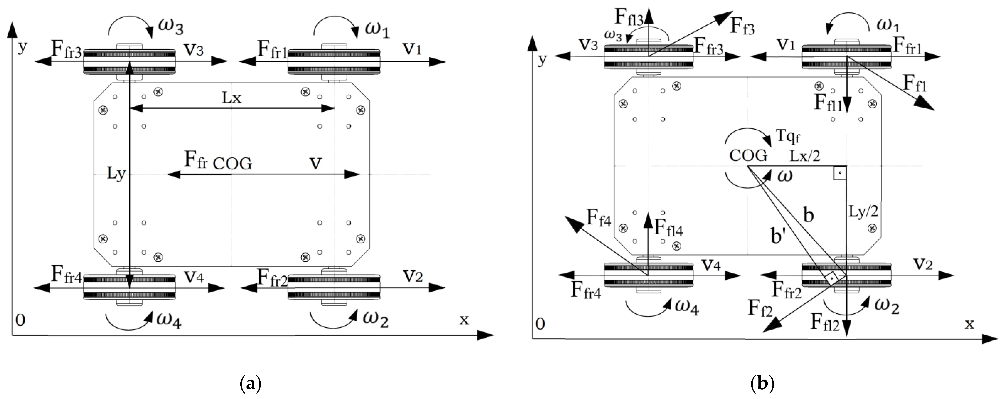
3.1.1. Forward and Backward Movement—Longitudinal Friction Force

This is the friction that occurs in the forward and backward movement. It is the friction experienced by traditional wheels and is crucial for propelling the robot in these directions [9,10,11,12,13].

A schematic representation of friction forces acting on a differential drive robot for linear movement is presented in Figure 1a. A representation of friction forces acting on a differential drive robot for rotational movement is presented in Figure 1b.

The equation for rolling friction force ${\mathrm{F}}_{\mathrm{f}\mathrm{r}}$ can be modeled using the classical model of friction force:

$${\mathrm{F}}_{\mathrm{f}\mathrm{r}}=-{\mathrm{\mu }}_{\mathrm{r}}·\mathrm{N}·\mathrm{s}\mathrm{g}\mathrm{n}\left({\mathrm{v}}_{\mathrm{X}}\right),$$

(13)

where ${\mathrm{\mu }}_{\mathrm{r}}$ is the rolling friction coefficient, and N is the normal force, which depends on the weight of the robot and its distribution on the wheels.

3.1.2. Rotational Movement

If it is presumed that the differentially driven mobile robot rotates around a central point, and its wheels exhibit varying movements, one can consider the forces of longitudinal friction as well as the lateral friction forces that arise during the rotation process [8,17].

Lateral direction friction force ${\mathrm{F}}_{\mathrm{f}\mathrm{l}}$ may arise from the speed difference between the left and right wheels during rotation. This lateral force may depend on the steering angle of the wheels and can be influenced by wheel slip. Because the lateral direction friction force is also similar to friction when sliding, one can assume the ${\mathrm{F}}_{\mathrm{f}\mathrm{l}}$ is:

$${\mathrm{F}}_{\mathrm{f}\mathrm{l}}=-{\mathrm{\mu }}_{\mathrm{s}}·\mathrm{N}·\mathrm{s}\mathrm{g}\mathrm{n}\left({\mathrm{v}}_{\mathrm{Y}}\right),$$

(14)

The total friction force ${\mathrm{F}}_{\mathrm{t}}$ during rotation can be the sum of the above forces:

$${\mathrm{F}}_{\mathrm{f}\mathrm{t}}={\mathrm{F}}_{\mathrm{f}\mathrm{r}}+{\mathrm{F}}_{\mathrm{f}\mathrm{l}}.$$

(15)

When a four-wheel drive robot rotates, both rolling friction and sliding (or lateral) friction come into play.

Modified model with rolling and lateral friction generates the total friction torque for rotation:

$${\mathrm{T}\mathrm{q}}_{\mathrm{f}}={-\mathrm{F}}_{\mathrm{f}\mathrm{t}}·\mathrm{b}·\mathrm{s}\mathrm{g}\mathrm{n}\left(\mathsf{\omega }\right),$$

(16)

$${\mathrm{T}\mathrm{q}}_{\mathrm{f}}={-(\mathrm{F}}_{\mathrm{f}\mathrm{r}}+{\mathrm{F}}_{\mathrm{f}\mathrm{l}})·\sqrt{{\frac{\mathrm{L}\mathrm{x}}{2}}^2+{\frac{\mathrm{L}\mathrm{y}}{2}}^2}\mathrm{s}\mathrm{g}\mathrm{n}(\mathsf{\omega }).$$

(17)

where b is the distance from the center of rotation to the wheel’s contact point with the rolling surface. For the friction forces coefficients, the models use ${\mathrm{\mu }}_{\mathrm{r}}$ = 0.05 and ${\mathrm{\mu }}_{\mathrm{s}}$ = 0.3.

These equations show that the lateral friction, which is dominant in this scenario, contributes significantly to the total frictional force and to the resulting torque required for rotation. The rolling friction, while present, has a smaller impact due to its typically lower friction coefficient. The above model provides a more comprehensive understanding of the friction forces during the rotation of a four-wheel drive mobile robot.

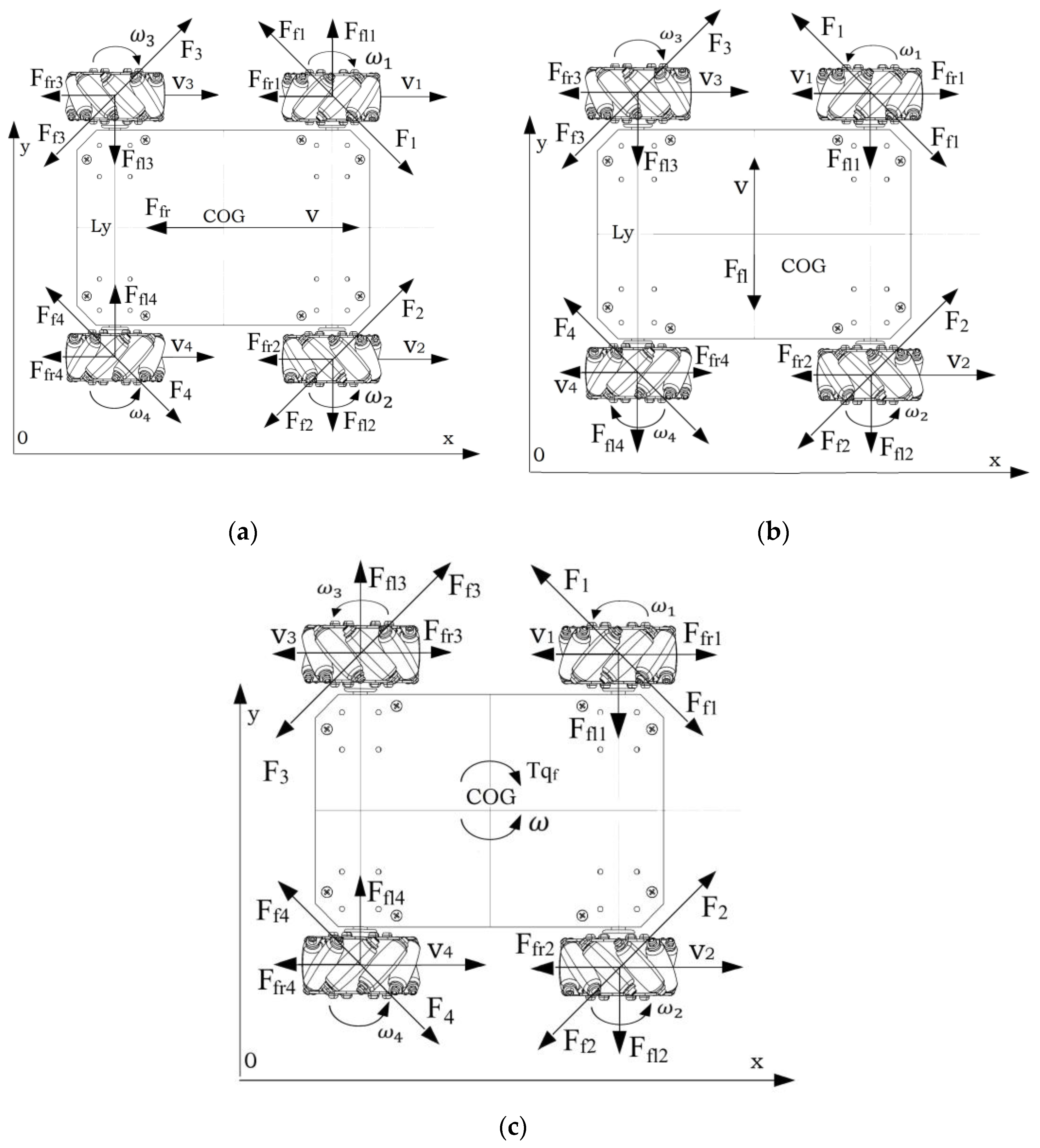
3.2. Friction Forces for Mecanum-Wheeled Mobile Robot

Here are key points regarding the friction of mobile robots equipped with Mecanum wheels. Mecanum wheels enable a robot to move in any direction—forward, backward, sideways, and diagonally—without changing the orientation of the robot. This is achieved by varying the direction and speed of rotation of each wheel. The rollers are typically mounted at a 45-degree angle to the wheel’s rotational axis. This angle is critical in determining the direction of frictional forces, which in turn affects the robot’s movement [21].

A schematic representation of friction forces acting on a Mecanum-wheeled robot for linear movement is presented in Figure 2a. A representation of friction forces acting on the robot for lateral movement is presented in Figure 2b and for rotational movement in Figure 2c.

For an enhanced mathematical model of a Mecanum-wheeled robot, it is crucial to incorporate both rolling and sliding friction, and to calculate the friction torque with distinctions between linear and rotational movements. The model must consider the roller’s angle $\mathsf{\alpha }$ in calculating sliding friction. Analyzing resistive friction between the Mecanum wheel and the ground is complex due to the robot’s omnidirectional movement and the wheel’s angled roller design. Each Mecanum wheel’s resistive friction is evaluated separately, involving both static and dynamic friction [21]. Static friction, present between stationary surfaces, must be overcome to initiate movement. Dynamic friction, occurring during relative motion between surfaces, must be overcome to maintain movement. Typically, the coefficient of static friction exceeds that of dynamic friction. Sliding friction ${\mathrm{F}}_{\mathrm{f}\mathrm{l}}$ arises when surfaces rub together, while rolling friction ${\mathrm{F}}_{\mathrm{f}\mathrm{r}}$ resists a wheel’s rolling motion on a surface.

Rolling friction for a Mecanum wheel is calculated as:

$${\mathrm{F}}_{\mathrm{f}\mathrm{r}}=-{\mathrm{\mu }}_{\mathrm{r}}·\mathrm{N}·\cos \left(\mathsf{\alpha }\right)·\mathrm{s}\mathrm{g}\mathrm{n}\left({\mathrm{v}}_{\mathrm{X}}\right),$$

(18)

where $\mathsf{\alpha }$ is the roller angle.

Sliding friction for a Mecanum wheel is calculated as:

$${\mathrm{F}}_{\mathrm{f}\mathrm{l}}=-{\mathrm{\mu }}_s·\mathrm{N}·\sin \left(\mathsf{\alpha }\right)·\mathrm{s}\mathrm{g}\mathrm{n}\left({\mathrm{v}}_{\mathrm{Y}}\right).$$

(19)

The direction depends on the wheel’s movement velocity (v) relative to the ground, projected along the roller in a parallel direction [21]. The advantage of the Mecanum wheel is that because of the roller, the sliding force imparts a rotational movement to the wheel’s roller, and thus the sliding force depends on the rolling friction force of the roller.

Friction Forces in Different Directions:

3.2.1. Forward and Backward Movement—Longitudinal Friction Force

This is the friction that occurs in the forward and backward movement. It is like the friction experienced by traditional wheels and is crucial for propelling the robot in these directions. Equation (13) also applies for this scenario.

Because of the roller angle, even in forward and backward movement the friction force has two components: longitudinal direction friction force and lateral direction friction force. However, in forward and backward movement, as shown in Figure 2c, the lateral friction forces cancel each other out.

$${\mathrm{F}}_{\mathrm{f}\mathrm{t}}={\sum }_{\mathrm{i}=1}^{\mathrm{n}}{\mathrm{F}}_{\mathrm{f}\mathrm{r}\mathrm{i}}+{\sum }_{\mathrm{i}=1}^{\mathrm{n}}{\mathrm{F}}_{\mathrm{f}\mathrm{l}\mathrm{i}},$$

(20)

where n is the number of wheels.

For forward movement, $\sum _{\mathrm{i}=1}^{\mathrm{n}}{\mathrm{F}}_{\mathrm{f}\mathrm{l}\mathrm{i}}$ = 0, so:

$${\mathrm{F}}_{\mathrm{f}\mathrm{t}}={\mathrm{F}}_{\mathrm{f}\mathrm{r}}.$$

(21)

3.2.2. Lateral Movement—Lateral Direction Friction Force

This friction comes into play when the robot moves sideways. It is significantly influenced by the design of the Mecanum wheels, particularly the angle and material of the rollers. In this case, the longitudinal friction forces cancel each other out, as shown in Figure 2c.

For side-to-side movement, $\sum _{\mathrm{i}=1}^{\mathrm{n}}{\mathrm{F}}_{\mathrm{f}\mathrm{r}\mathrm{i}}$ = 0, so:

$${\mathrm{F}}_{\mathrm{f}\mathrm{t}}={\mathrm{F}}_{\mathrm{f}\mathrm{l}}.$$

(22)

3.2.3. Rotational Movement

The friction in this case has both a longitudinal and lateral component, so $\sum _{\mathrm{i}=1}^{\mathrm{n}}{\mathrm{F}}_{\mathrm{f}\mathrm{l}\mathrm{i}}$ and $\sum _{\mathrm{i}=1}^{\mathrm{n}}{\mathrm{F}}_{\mathrm{f}\mathrm{r}\mathrm{i}}$ are different from zero. Because the lateral friction forces in the case of Mecanum wheels induce a rotational motion of the wheel’s roller around its own axis, the lateral friction forces through the wheel’s rollers have a characteristic like rolling friction. In this case, the friction force can also be approximated to:

$${\mathrm{F}}_{\mathrm{f}\mathrm{t}}={\mathrm{F}}_{\mathrm{f}\mathrm{r}}+{\mathrm{F}}_{\mathrm{f}\mathrm{l}}.$$

(23)

Total friction torque for rotation:

$${\mathrm{T}\mathrm{q}}_{\mathrm{f}}={\mathrm{F}}_{\mathrm{f}\mathrm{t}}·\mathrm{b},$$

(24)

$${\mathrm{T}\mathrm{q}}_{\mathrm{f}}={-\mathrm{\mu }}_{\mathrm{r}}·\mathrm{N}·\sqrt{{\frac{\mathrm{L}\mathrm{x}}{2}}^2+{\frac{\mathrm{L}\mathrm{y}}{2}}^2}·\mathrm{s}\mathrm{g}\mathrm{n}(\mathsf{\omega }).$$

(25)

The frictional characteristics of Mecanum wheels are complex and multifaceted, playing a crucial role in the omnidirectional mobility of robots. The design and material of the wheels, along with the surface characteristics, significantly impact the robot’s movement and control.

4. Dynamics of Wheeled Mobile Robots

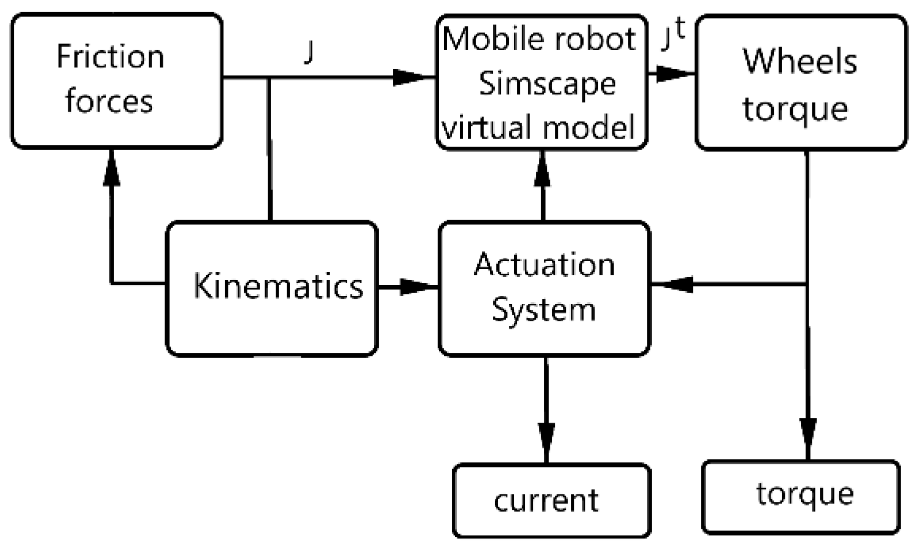
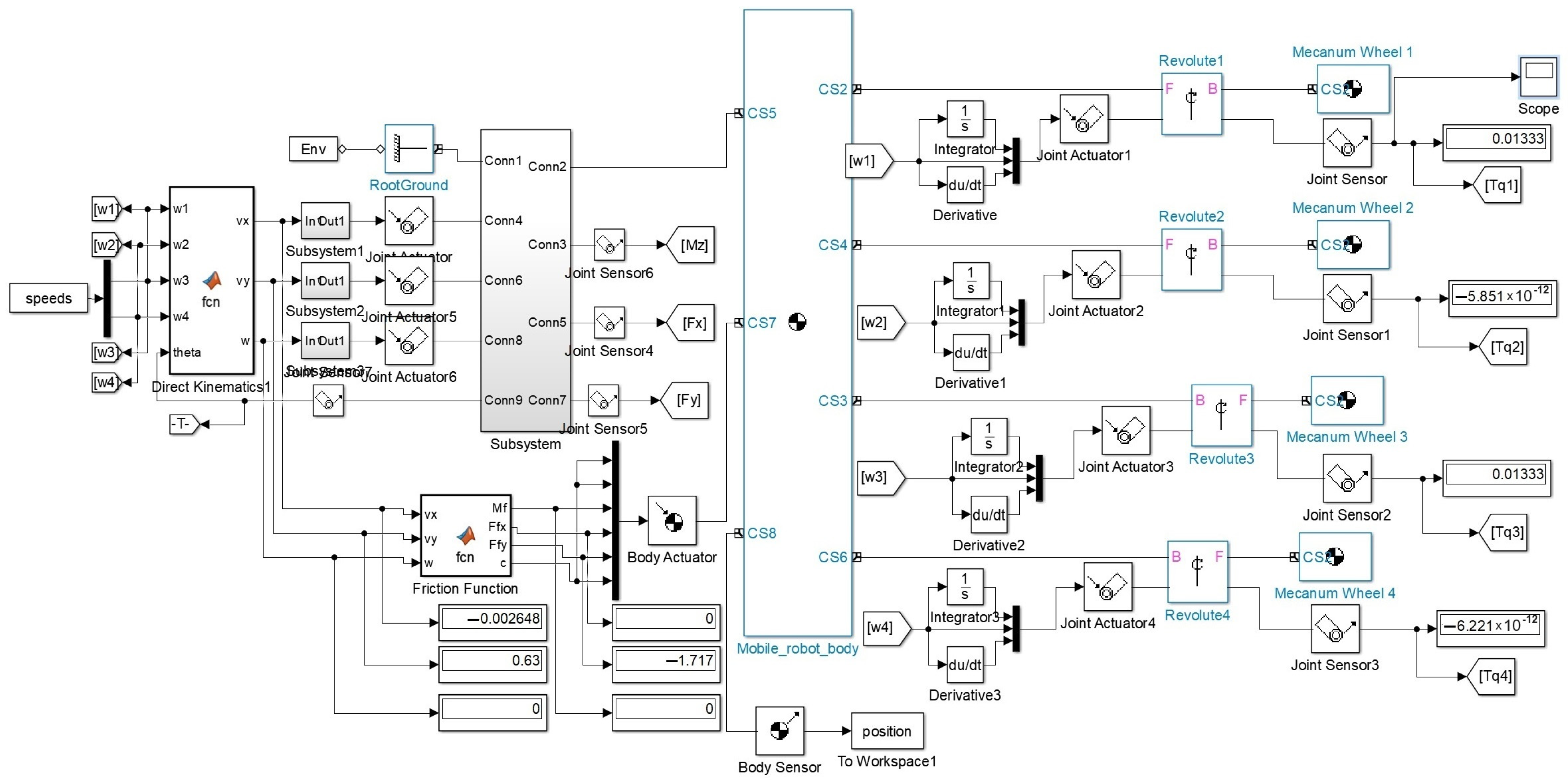
The dynamic model of a mobile platform was developed within the Simulink environment. This dynamic model was based on importing a three-dimensional virtual assembly model from SolidWorks and was entirely modeled within the Simulink–Simscape environment.

The model includes the following key elements:

• Kinematic Actuation Block: This functional block in Simulink controls the motion of the kinematic elements of the mobile platform, enabling it to move and perform various actions based on commands and inputs.
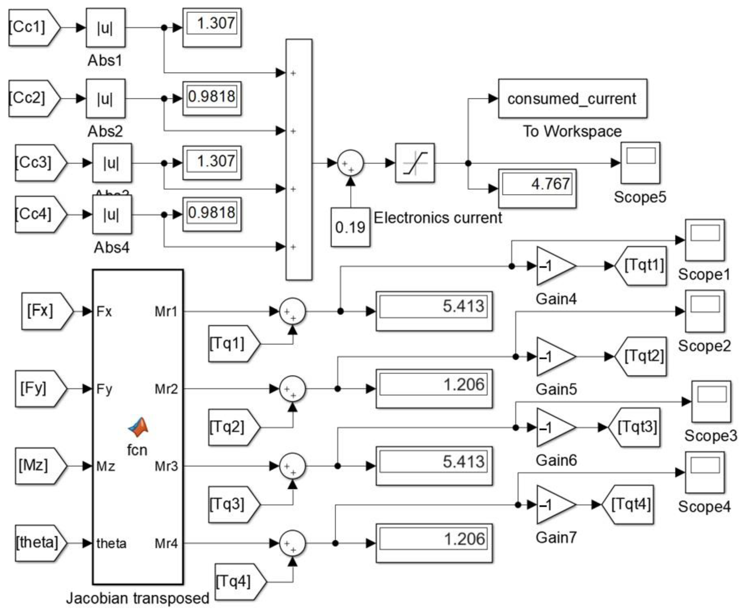
• Transpose Jacobian Matrix Block: This functional block calculates the transposed Jacobian matrix of the mobile platform, providing essential insight into the relationship between the joint torques and the resistive forces acting on the robot body.
• Friction Force Integration Block: This functional block deals with integrating friction forces into your dynamic model, ensuring a realistic simulation of the mobile platform’s motion.
• Simscape Model: Additionally, it is worth noting that the entire dynamic model of the mobile platform is created within the Simulink Simscape environment, making it a powerful and versatile solution for simulating and analyzing the platform’s behavior.

By implementing these functional blocks within the Simulink environment, one can create a complex dynamic model of a mobile platform, providing a solid foundation for testing, improving, and analyzing its behavior in a controlled virtual environment. This model can be invaluable in the development and optimization of mobile platforms.

The dynamic model block diagram is presented in Figure 3.

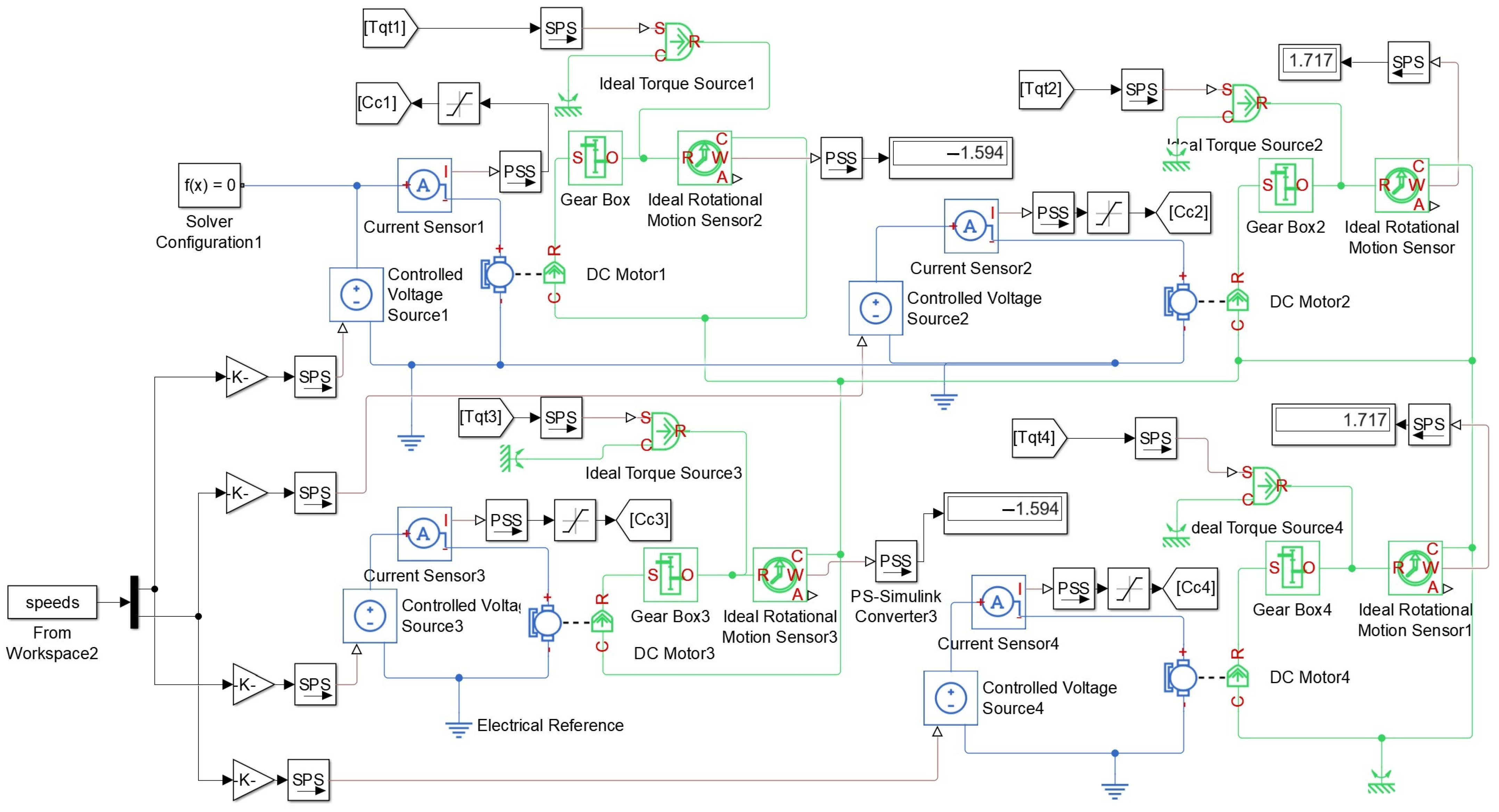
In the following section, the complex system designed to simulate the motion control of a mobile robot that considers the kinematics, dynamics, and the influence of frictional forces on the robot’s movement and power consumption is presented. The block diagram for the entire dynamic model of the mobile robot is represented in Figure 4, Figure 5 and Figure 6.

5. Physical Model

The mobile robot used for validating the dynamic model is a mechatronic platform, designed with relatively high-performance components that work together to ensure its efficient and precise operation.

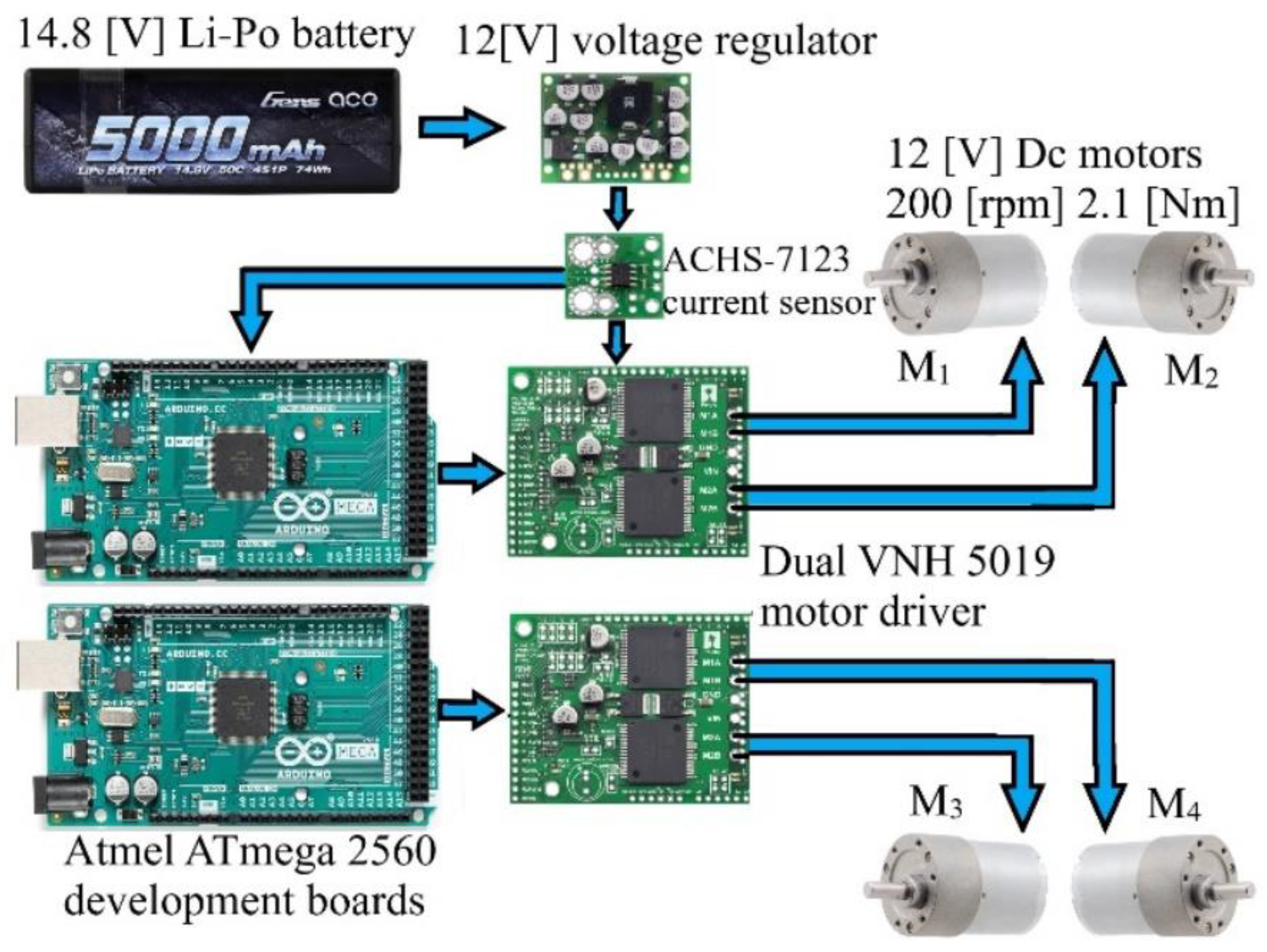
The robot’s control system was built around two microcontroller development boards with an AT Mega 2560 controller (Microchip, Chandler, AZ, USA). These boards were chosen for their high processing power and extensive array of input/output pins, making them ideal for complex robotic applications. They offer a significant improvement over development boards in terms of I/O capabilities and processing power, essential for managing multiple sensors and motor controls.

For motion control, the robot uses two DualVNH5019 (Pololu Robotics and Electronics, Las Vegas, NV, USA) motor driver shields. These high-power motor drivers can operate from 5.5 to 24 V and deliver a continuous 12 A (30 A peak) per motor, or 24 A (60 A peak) to a single motor when combined. They offer current-sense feedback, accept high PWM frequencies for quieter operation, and are equipped with a variety of protection features such as reverse-voltage protection, thermal shutdown, and short-circuit protection.

The robot is actuated by four 12 V DC motors, each capable of reaching a maximum speed of 200 RPM. These motors are controlled by the DualVNH5019 motor driver shields, allowing for precise and responsive movement.

Powering the robot is a D24V150Fx (Pololu Robotics and Electronics, Las Vegas, NV, USA) family step-down voltage regulator, which is a high-current synchronous switching regulator that efficiently generates lower output voltages from input voltages as high as 40 V. It has an efficiency of 80% to 95%, an instantaneous current limit of approximately 32 A, and can typically support continuous output currents between 5 A and 20 A.

The robot’s power system includes a 14.8 V Li-Po battery, coupled with a 12 V, 15 A voltage regulator, ensuring stable and adequate power for the motors and electronic components.

To monitor the robot’s power consumption, an ACHS-7123 (Pololu Robotics and Electronics, Las Vegas, NV, USA) current sensor was integrated into its circuit. This sensor can handle a bidirectional current input up to 30 A and outputs a proportional analog voltage. It features low internal resistance (~0.7 mΩ), electrical isolation up to 3 kV RMS, a bandwidth of 80 kHz, high accuracy, and a wide operating temperature range (−40 °C to 110 °C).

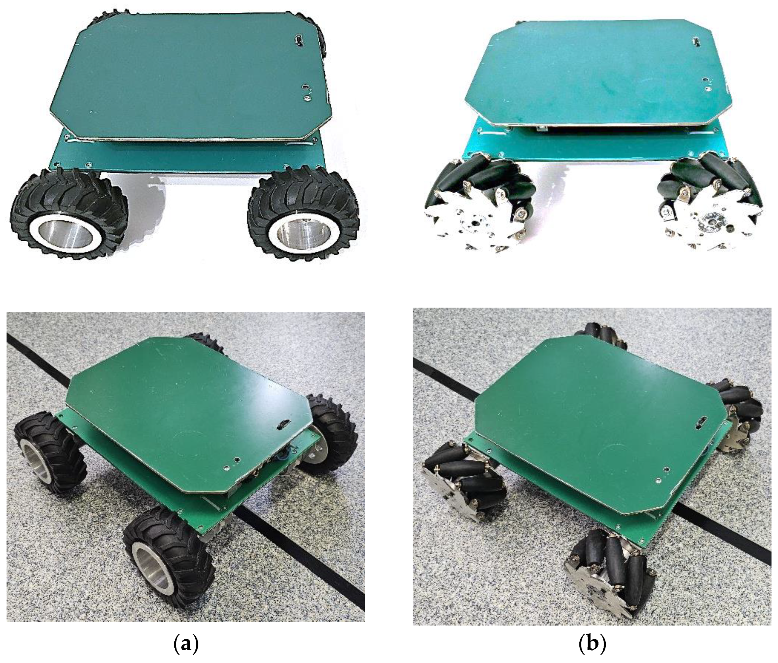
The mobile robot used for validating the dynamic model in the differential drive configuration is presented in Figure 7a, and that used to validate the omni drive configuration is presented in Figure 7b.

The components used for developing the mobile platform are presented in the electronic diagram below; see Figure 8.

6. Cost Function for Energy Consumption Estimation

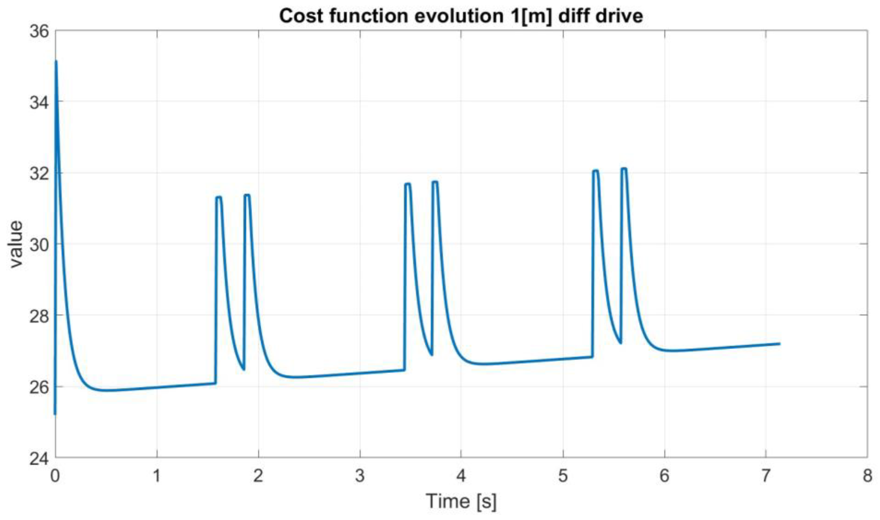
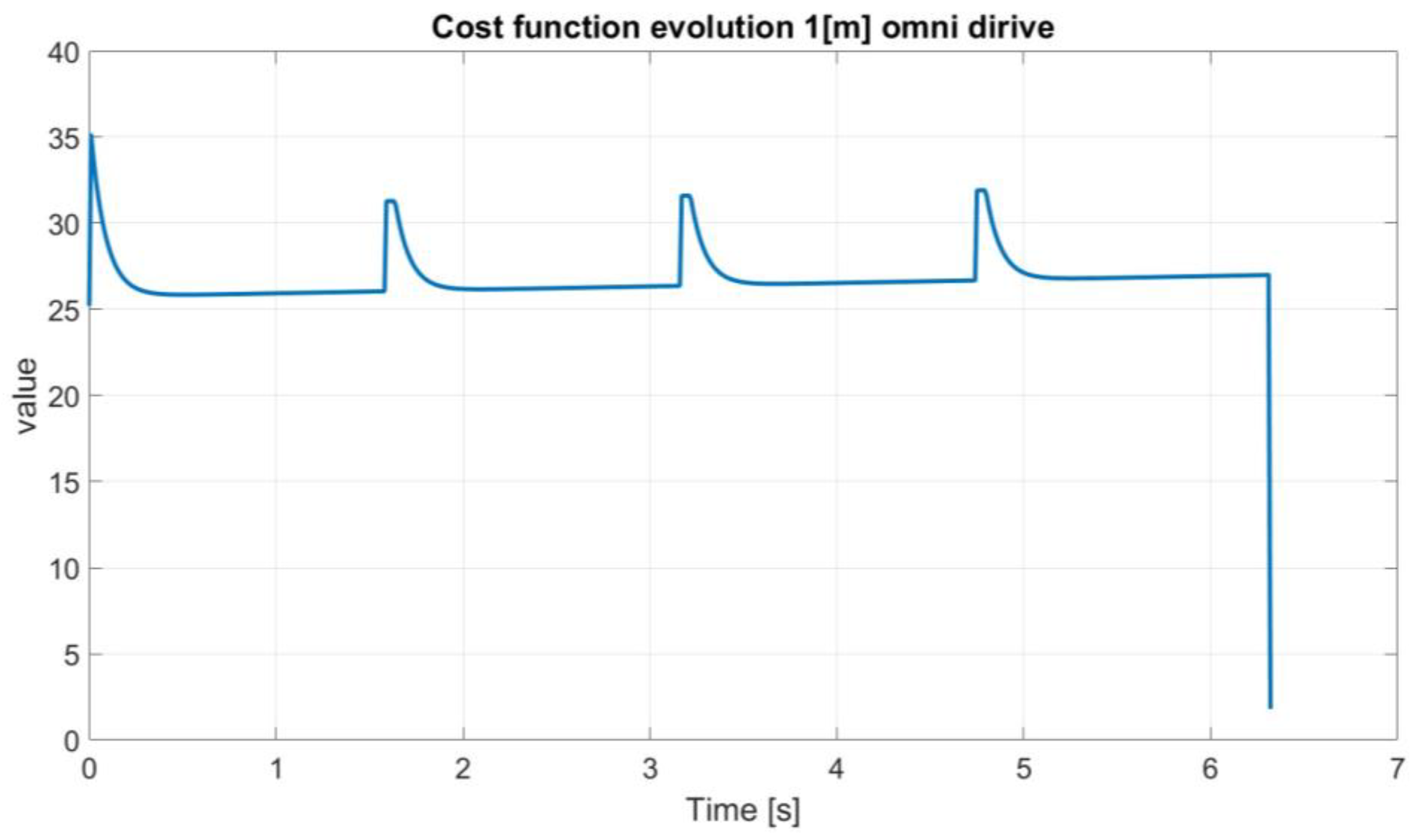
In this section, particular attention is given to the cost function, which is an essential aspect in choosing the driving mode for the omnidirectional mobile robot. The cost function is designed to consider multiple variables such as current consumption, velocity, trajectory tracking accuracy, or other performance criteria. By creating this cost function, the overall performance of the robot can be improved in terms of energy efficiency and motion precision. Thus, the analysis and adjustment of the cost function are crucial elements in the design and implementation process of the control system for the omnidirectional mobile robot.

In this research, the significance of the cost function lies solely in making decisions regarding the operational mode of the mobile robot, with no emphasis on path planning algorithms. By employing the cost function, one can determine the relative efficiency of the robot’s locomotion mode for a given type of movement, Figure 9 and Figure 10.

Here are the steps used to build the cost function:

Defining Parameters:

-

Inputs:

• currentConsumption—Vector containing the current consumed by each wheel’s motor (amps);
• wheelRotations—Vector containing the total number of rotations for each wheel;
• elapsedTime—Total time taken to complete the trajectory (seconds);
• wCurrent, wRotations, wTime—Weights for current consumption, wheel rotations, and time.

-

Output:

• totalCost—Calculated total cost of the trajectory based on the inputs and weights;
• currentCost = sum(currentConsumption); the sum of all current consumed;
• rotationCost = sum(wheelRotations); the sum of all wheel rotations;
• timeCost = elapsedTime; the total time.

Computing the weighted sum of costs:

C = wCurrent × currentCost + wRotations × rotationCost + wTime × timeCost

(26)

Example for the cost function implemented into a MATLAB function block:

function totalCost = calculateTrajectoryCost(currentConsumption, wheelRotations, elapsedTime, wCurrent, wRotations, wTime)

totalCost = wCurrent × currentCost + wRotations × rotationCost + wTime × timeCost;

end

The total value of the function for differential driving is totalCost = 19,411 and the total value of the function for omnidirectional driving is totalCost = 16,948. So, for this type of imposed trajectory, the omnidirectional driving mode is more efficient. These data will be used as input into the fuzzy logic decision block for a specific driving mode.

This approach can be adjusted and refined based on the specific characteristics of the robot and the complexity of the environment in which it operates.

7. Decision-Making in Driving Mode Using Fuzzy Logic

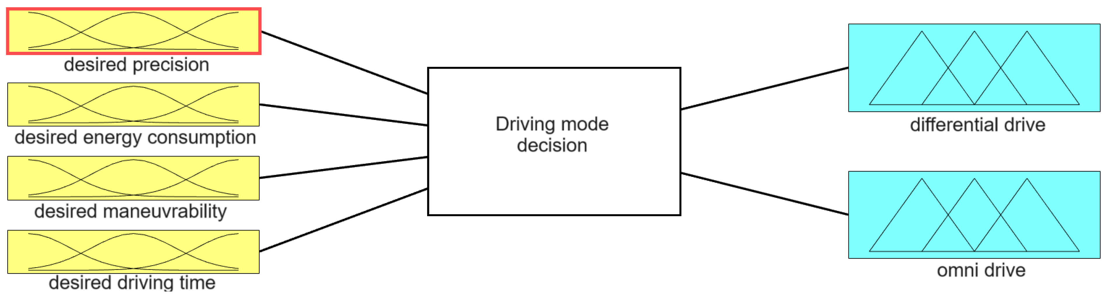
This section presents the development of a fuzzy logic model for decision-making in trajectory driving mode for a Mecanum-wheeled mobile robot. The model considers four key input variables: desired precision, energy consumption goals, maneuverability preferences, and specified trajectory driving time, each classified as either low or high. Output variables, representing differential drive and omnidirectional drive, are determined through ten fuzzy rules derived from these inputs.

Fuzzy logic significantly enhances the precision of positioning in autonomous mobile robots, serving as a tool for advanced control systems that require refined decision-making. This approach is particularly valuable when robots operate in environments where exact positioning is critical, but direct measurements are not possible. Fuzzy logic enables these systems to interpret and make sense of imprecise sensor data, facilitating more accurate estimations of the robot’s current location [12,13,14].

By processing a range of inputs as fuzzy sets—essentially degrees of truth rather than binary on/off signals—robots can adjust their movements in real time to align more closely with the desired position [22,23,24,25,26]. This capability is crucial for tasks that demand high levels of accuracy, such as assembly in manufacturing or precise navigation in tightly constrained spaces. Through the application of fuzzy logic, robots are not just reacting to their environment but are actively interpreting it, allowing for adjustments that refine their positioning to a degree of precision previously unattainable with traditional binary control systems [29,32,39,42].

This paper introduces a fuzzy decision algorithm designed to determine the most suitable motion mode for Mecanum wheel-equipped mobile platforms. This innovative approach enables informed decision-making by balancing efficiency, speed, and operational demands, thereby enhancing the platform’s adaptability and performance in diverse environments. By focusing on driving mode decisions, this research addresses a gap in the current mobile robot domain, offering a novel perspective in the field of mobile robotics.

Using fuzzy logic, the algorithm evaluates these parameters simultaneously, incorporating linguistic variables and considering their relative importance and task-specific requirements. By employing a set of fuzzy rules, the algorithm provides output data that guide motion mode selection, ensuring an adaptable and comprehensive approach to optimizing energy consumption and maneuverability under varying operational conditions and constraints. This innovative method shifts focus towards driving mode decisions, addressing a gap in the current research emphasis on trajectory precision, and enhancing the platform’s performance and adaptability in diverse environments.

Membership functions for inputs (desired precision, desired energy consumption, desired maneuverability, desired time):

Desired precision:

LOW: Triangular, with values around 0.0 and 0.5.

HIGH: Triangular, with values around 0.5 and 1.0.

Desired energy consumption:

LOW: Triangular, with values around 0.0 and 0.5.

HIGH: Triangular, with values around 0.5 and 1.0.

Desired maneuverability:

LOW: Triangular, with values around 0.0 and 0.5.

HIGH: Triangular, with values around 0.5 and 1.0.

Desired time:

LOW: Triangular, with values around 0.0 and 0.5.

HIGH: Triangular, with values around 0.5 and 1.0.

Membership functions for outputs (differential locomotion, omnidirectional locomotion):

Differential locomotion:

LOW: Triangular, with values around 0.0 and 0.5.

HIGH: Triangular, with values around 0.5 and 1.0.

Omni locomotion:

LOW: Triangular, with values around 0.0 and 0.5.

HIGH: Triangular, with values around 0.5 and 1.0.

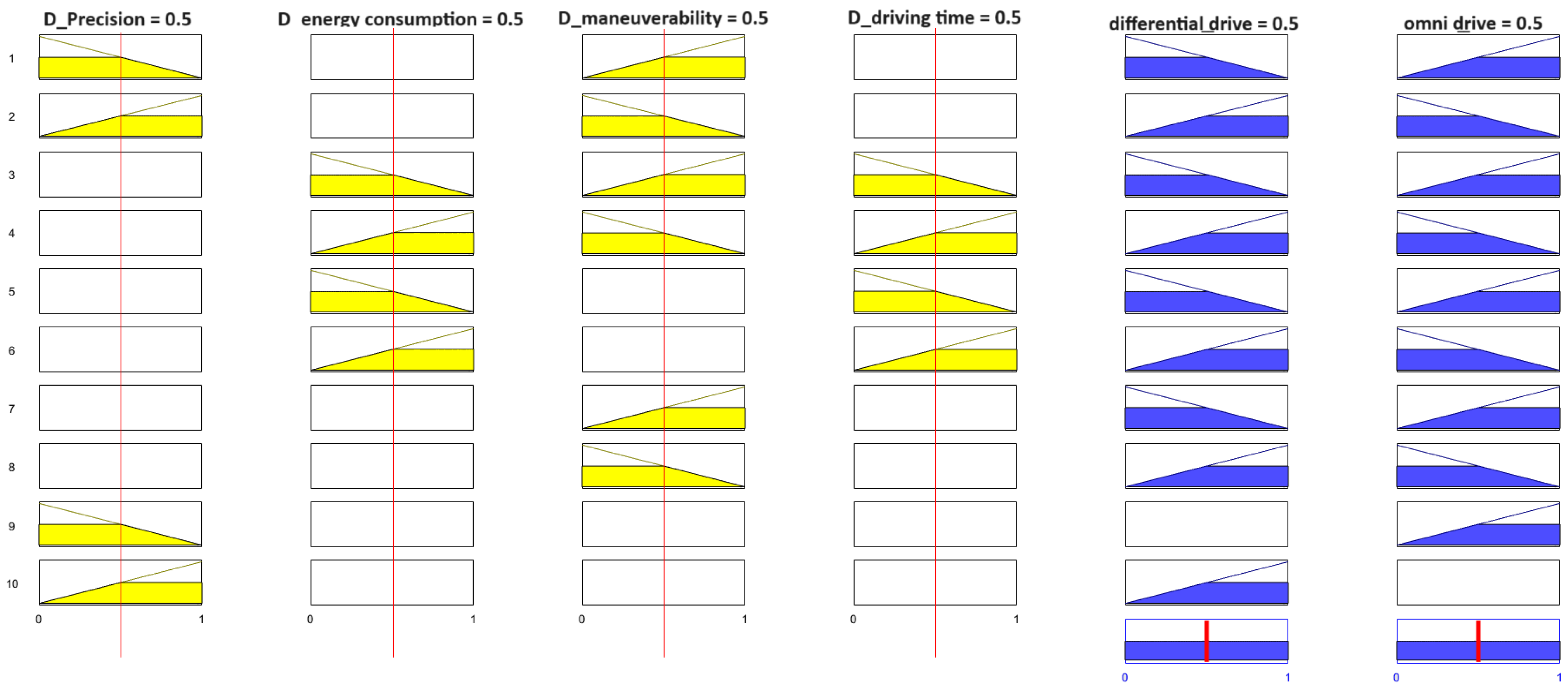
The fuzzy logic rules are based on these assumptions: When precision is high and maneuverability is prioritized, the model suggests omnidirectional drive. In contrast, high precision with low maneuverability favors differential drive. Low energy consumption, high maneuverability, and short traversal times support omnidirectional drive. High energy consumption, low maneuverability, and lengthy traversal times lean towards differential drive. Low energy consumption and short traversal times are indicators for omnidirectional drive. High energy consumption coupled with extended traversal times favors differential drive. Enhanced maneuverability encourages omnidirectional drive. In contrast, limited maneuverability leads to differential drive. High precision requirements suggest differential drive. In contrast, low precision requirements recommend omnidirectional drive. These rules guide the fuzzy logic model in making decisions regarding the optimal trajectory traversal method, contributing to advancements in autonomous mobile robotics engineering, Figure 11 and Figure 12.

The fuzzy rules are presented below:

• If (D__precision is LOW) and (D__maneuverability is HIGH) then (differential__drive is LOW)(omni__drive is HIGH)
• If (D__precision is HIGH) and (D__maneuverability is LOW) then (differential__drive is HIGH)(omni__drive is LOW)
• If (D__energy__consumption is LOW) and (D__maneuverability is HIGH) and (D__driving__time is LOW) then (differential__drive is LOW)(omni__drive is HIGH)
• If (D__energy__consumption is HIGH) and (D__maneuverability is LOW) and (D__driving__time is HIGH) then (differential__drive is HIGH)(omni__drive is LOW)
• If (D__energy__consumption is LOW) and (D__driving__time is LOW) then (differential__drive is LOW)(omni__drive is HIGH)
• If (D__energy__consumption is HIGH) and (D__driving__time is HIGH) then (differential__drive is HIGH)(omni__drive is LOW)
• If (D__maneuverability is HIGH) then (differential__drive is LOW)(omni__drive is HIGH)
• If (D__maneuverability is LOW) then (differential__drive is HIGH)(omni__drive is LOW)
• If (D__maneuverability is LOW) then (differential__drive is HIGH)(omni__drive is LOW)
• If (D__precision is HIGH) then (differential__drive is HIGH)

8. Validating the Simulink Dynamic Models of the Robot

This section provides a description of the experimental results, their interpretation, and the experimental conclusions that can be drawn.

Measurements were taken for various movements of the mobile robot, followed by minor adjustments to the robot’s dynamic model. The dynamic model in Simulink, as mentioned earlier, is necessary when it comes to optimizing the robot for specific missions in its workspace. The following experimental trials were conducted to validate the dynamic models in Simulink:

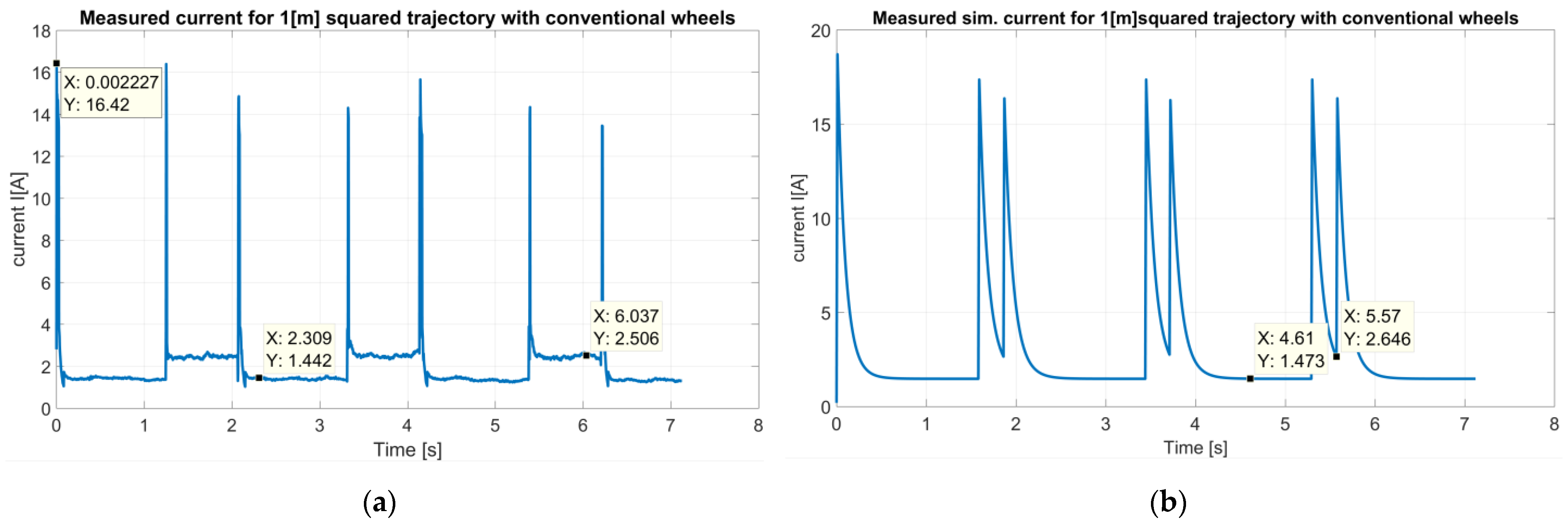
8.1. Measured Current following 1 [m] Squared Trajectory with Conventional Wheel Configuration

The two graphs presented in Figure 13a,b show the current consumption profiles for the mobile robot following a 1 m square trajectory using a conventional wheel design. Figure 13a shows real-world measurements and Figure 13b shows simulated measurements using a Simulink Simscape dynamic model.

In Figure 13a, the current profile shows several peaks, which correspond to moments when the robot changes direction or accelerates, requiring more power from the motors. The highest peak reaches approximately 16.42 A in the measurement, suggesting an initial surge in current, due to the robot starting motion from rest and overcoming initial static friction. Other notable values occur at 1.442 A and 2.506 A, indicating the forward movement and the rotation of the robot, which are the steady-state currents required to maintain motion. These currents are the result of kinematic friction forces.

In Figure 13b, the simulated current consumption using the dynamic model created in Simulink Simscape is presented. Like the real measurement, the profile consists of sharp spikes in current consumption. The peaks appear at regular intervals, consistent with the square trajectory pattern, and they seem slightly higher than the real-world measurements. The simulation includes the robot’s dynamic model, motor characteristics, and the friction forces that the robot encounters. As expected, the simulation shows a smoother curve without the noise and minor fluctuations present in the actual measurements, as real-world factors like motor efficiency, and surface irregularities are difficult to model precisely. The occurrence of peaks at consistent intervals suggests that the dynamic model is accurately capturing the moments when the robot requires more current, such as starting, stopping, or turning.

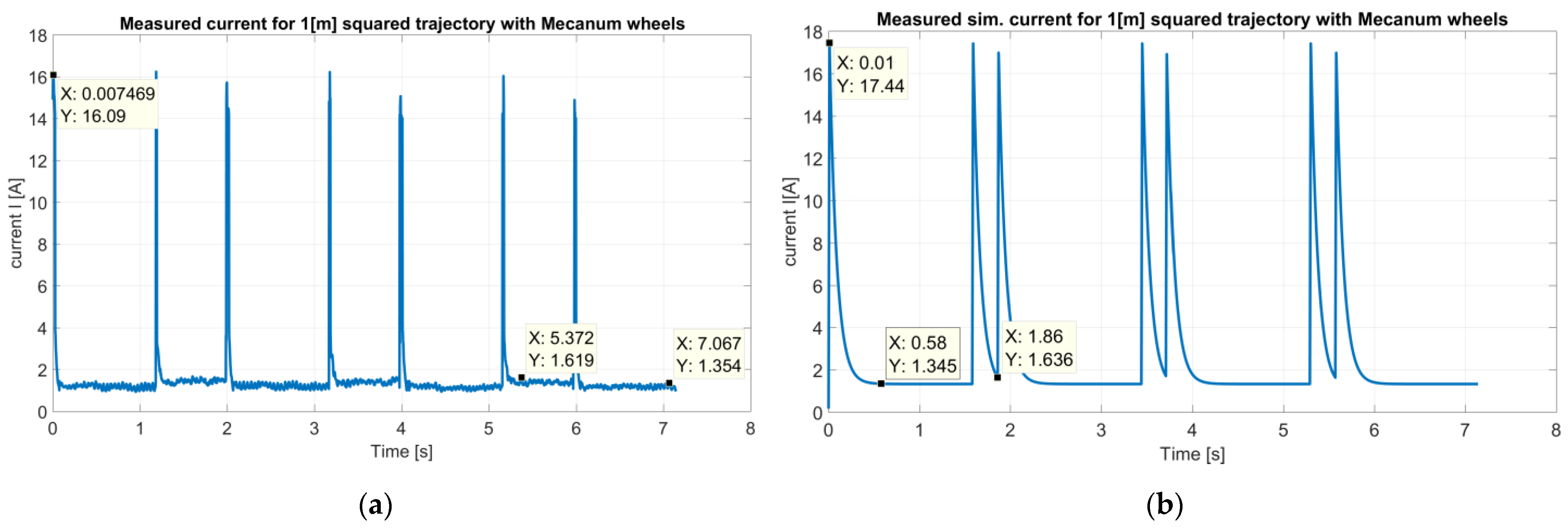
8.2. Measured Current for 1 [m] Squared Trajectory with Mecanum Wheel Configuration

The two graphs presented in Figure 14a,b show the current consumption profiles for the mobile robot following a 1 m square trajectory using Mecanum wheels, with the graph in Figure 14a showing real-world measurements and the graph in Figure 14b showing simulated measurements using a Simulink Simscape dynamic model.

Based on the provided graphs, one can draw several conclusions. Both graphs show significant peaks in current at certain points, which are likely to correspond with the robot’s maneuvers, such as turning at the corners of the square trajectory. In the first graph in Figure 14a, the highest peak occurs very early, at 0.007469 s, with a current of 16.09 A. Similarly, in the graph shown in Figure 14b, the first peak is also at the beginning, around 0.01 s, with a slightly higher current of 17.44 A. The timing of the peaks in both graphs suggests that the robot experiences the highest current draw at similar instances during the trajectory. However, there is a slight timing difference, with the simulated data showing a slightly earlier peak. This can be attributed to the absence of real-world delays in the simulation. Both graphs display four distinct peaks, which match the four corners of the square trajectory where the robot changes direction. The magnitudes of the peaks in both graphs vary. In the experimental graph shown in Figure 14a, the peaks following the initial one have lower values, whereas in the simulated graph shown in Figure 14b, the subsequent peaks have similar magnitudes to the first peak. The steady-state current, or the current level between the peaks, appears to be consistent in both graphs, indicating that the simulation can accurately model the robot’s power consumption during non-maneuvering phases. The shapes of the curves in both graphs are similar, with sharp increases and decreases in current, reflecting the dynamic response of the robot’s electrical system to the maneuvers. The simulated graph in Figure 14b has smoother transitions, which is typical for simulated data that do not include the noise or variability found in experimental measurements. Figure 14a shows more variability and noise, as expected from real-world measurements where factors such as sensor precision, battery voltage fluctuations, and varying resistance can affect the readings.

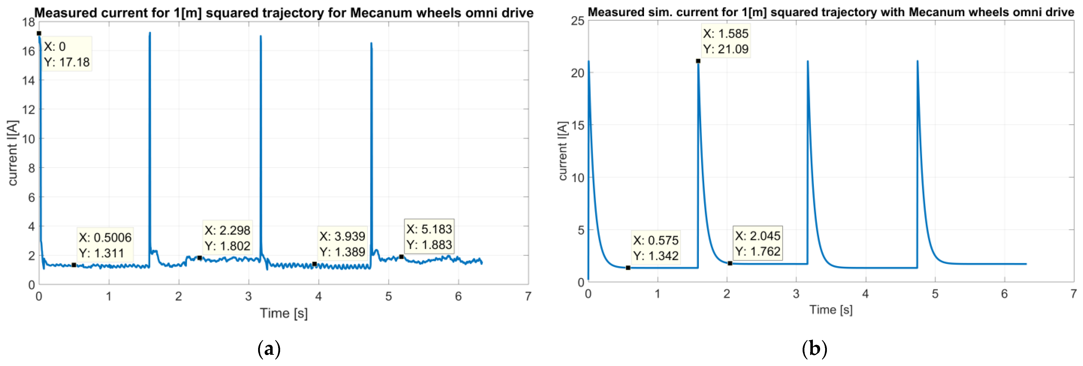
8.3. Measured Current for 1 [m] Squared Trajectory with Mecanum Wheel Configuration and Omnidirectional Drive

The two graphs presented in Figure 15a,b show the current consumption profiles for the mobile robot following a 1 m square trajectory using a Mecanum wheel design and omni drive locomotion. The graph in Figure 15a shows real-world measurements. The graph from Figure 15b shows simulated measurements using a Simulink Simscape dynamic model.

Comparing the data from the two, it can be seen that both graphs feature prominent peaks indicative of high current demands at specific points in the trajectory. The graph from Figure 15a starts with a peak at time X: 0 s, with a current of 17.18 A, which is a typical surge at the start of motion. The graph presented in Figure 15b shows a similar initial surge, peaking at 21.09 A at X: 1.585 s, which is significantly higher than the experimental peak. The peaks in Figure 15b occur at regular intervals, suggesting a consistent pattern of behavior such as moving sideways onto the imposed trajectory. In Figure 15a, the peaks also follow a regular pattern, but they appear slightly less evenly spaced compared to the simulated data. Between the peaks, Figure 15a shows a relatively steady current, suggesting consistent demand when the robot is not changing direction. Figure 15b exhibits a similar behavior, but with a more pronounced drop to a lower current between the peaks, suggesting that the simulation may not fully account for all the real-world resistive forces acting on the robot. Both graphs illustrate the trend of high current demands at the beginning and at points that likely correspond to maneuvers or accelerations. The trends in the current demand over time are generally similar, which indicates that the simulation is modeling the key aspects of the robot’s motion and electrical demand. The experimental data in Figure 15a display variability in the height of the current peaks after the initial surge, which may reflect the complex interactions between the robot’s drive system and the environment. The simulated data in Figure 15b show less variability in peak heights, with most peaks reaching similar maximum current levels. Figure 15a might exhibit more noise and minor fluctuations than Figure 15b, which is common in real-world measurements due to factors like sensor precision and environmental inconsistencies.

Following the simulation runs and experimental trials, one can draw the following conclusions: Upon monitoring the current consumption resulting from the experimental trials and comparing it with the currents obtained from the simulation, it can be clearly stated that the dynamic models in Simulink are accurately constructed, and the forces acting on the mobile platform are mathematically well modeled. From the experimental trials, it was observed that the mobile platform, using omnidirectional locomotion, did not drive through the trajectories with high precision; lateral movement led to deviations from the imposed trajectory. The driving time of the trajectory was relatively shorter In the case of omnidirectional movement compared to when the robot moved differentially, but the timing differences were very small. These aspects will be taken into account when deciding the type of locomotion for driving the robot onto a predefined trajectory.

9. Conclusions

This study presents significant practical implications for the design of mobile platforms, emphasizing the importance of selecting suitable driving types and control strategies designed to specific operational requirements such as energy efficiency, terrain traversal, and maneuverability. By developing and validating a dynamic model for mobile platforms, particularly those equipped with Mecanum wheels, this paper offers valuable insights into optimizing their design and control systems.

This research contributes to the robotics field by introducing a comprehensive approach to understanding and enhancing the dynamics and control of autonomous mobile robots. Unlike traditional methods relying on differential equations, this study employs Simulink’s block-based diagrams for a simplified development process. Notably, the dynamic model incorporates friction forces on the wheels, crucial for accurate energy monitoring.

Through experimental validation, this study ensures the accuracy and reliability of the dynamic model. Moreover, it explores the integration of 3D models from SolidWorks into Simulink, enabling detailed representations of mobile platforms. By formulating mathematical models for both conventional and Mecanum wheel configurations, the paper facilitates the development of energy-efficient driving strategies.

The decomposition of resistive forces using the Jacobian matrix enables precise simulation of electrical current consumption during robot motion. This paper’s focus on energy consumption monitoring and trajectory tracking, coupled with fuzzy decision algorithms, proposes a method for determining optimal locomotion modes for Mecanum wheel-equipped mobile platforms.

As elements of novelty, this paper presents the development of a dynamic model for mobile platforms based on importing a 3D assembly into Simscape-Multibody. The dynamic model considers the friction forces acting on the wheels. Different scenarios in which friction forces occur and act on the mobile platform have been analyzed and described in detail: front–back differential motion and rotation, front–back omnidirectional motion, rotation, and lateral motion. This analysis and description of wheel friction forces are novel elements because few works detail these five cases of locomotion. The detailed description of friction forces is crucial because friction is the component of resistance forces that distinguishes the energy consumption between different locomotion types the most. If this friction force model were not correctly modeled, the energy consumption for the five types of movement would not show significant differences. The dynamic model and the friction forces model were experimentally validated, and this aspect was presented in Section 8.

The dynamic model of the mobile platform is necessary for a user to identify the energy consumption for specific locomotion types. The cost function is important in monitoring energy consumption.

A fuzzy logic-based model necessary and useful in selecting a locomotion mode for a particular trajectory has been developed. Based on input parameters such as desired energy consumption, desired displacement accuracy, necessary mobility, and travel time, a trajectory can be divided into several sectors, and the robot can use different locomotion modes for each sector. This research does not focus on controlling and precisely tracking the imposed trajectory because numerous works present these aspects. The novelty lies in choosing the driving mode of the imposed trajectory.

As future work, improving the fuzzy model and testing the entire process on a trajectory of high complexity is proposed.

In conclusion, this research significantly advances the field of autonomous mobile robotics by providing a comprehensive framework for dynamic modeling and energy-efficient operation. The experimental validation of dynamic models and thorough analysis of resistive forces promise substantial progress in the practical implementation of autonomous mobile platforms.