Adaptive Prosthetic Trajectory Estimation Based on Key Points Constraints

Abstract

Lower limb knee–ankle prostheses can effectively assist above-knee amputees in completing their basic daily activities. This study explored methods for estimating the joint kinematics of intelligent lower limb prostheses to better adapt them to the walking requirements of amputees. A method of estimating the knee and ankle joint trajectories under different speeds and slopes was raised. The joints of a prosthetic need to have a movement trajectory similar to that of the joints of healthy individuals, taking into account the person’s motion intentions and complying with the law of movement. In this study, a prosthetic kinematics estimation method was studied to realize continuous speed and slope adaptation through key points. The iterative Douglas–Peucker algorithm automatically found the key points of the kinematic trajectory curve, and an invariant basis function-fitting model with key points constraints was constructed. Finally, the radial basis function neural network was used to estimate the adaptive task function of the parts affected by the speed and slope, resulting in an overall kinematics estimation model. Our experiments verified the effectiveness of the proposed method, which accurately estimated the kinematic trajectory; the knee and ankle joint estimation errors were greatly reduced compared to those obtained with previous methods, facilitating further research on individual algorithms.

1. Introduction

Lower limb knee–ankle prostheses are commonly used devices that can effectively assist above-knee amputees in completing their basic daily activities and lead to significant social and economic benefits. Intelligent prostheses can actively perform the relevant actions and allow the prosthetic side to match the healthy side better [1,2,3]. The joint biomechanical characteristics of prosthetics are designed to be more in line with the characteristics of healthy people, ensuring safety and comfort during walking. Prostheses remain in close contact with the wearer, which is an important application in the field of human–robot interaction (HRI). While the development of intelligent technology has improved the performance of such systems to a certain extent, it still has limitations in dynamic and complex environments and tasks [4]. One aspect is the research on controllers, with user comfort as the core. Current prosthetic research primarily focuses on achieving prosthetic control performance, often overlooking the crucial aspect of comfort. Research should prioritize comfort as the main indicator. Secondly, there is the accurate expression and recognition of the wearer’s motion intent. The wearer’s subjective will should serve as the primary source of control commands in the human–prosthesis interaction system. Therefore, it is essential to accurately determine the wearer’s current motion intent and design appropriate intent command information to transmit to the prosthetic controller.

The kinematic estimation of a prosthesis involves calculating and optimizing its motion trajectory based on information about the user’s intentions and motion states. This ensures that the prosthesis matches the gait cycle and stride length of healthy individuals, while also avoiding noticeable impacts or vibrations that could make the walking process uncomfortable. To achieve this, a kinematic model is established for both the prosthesis and the human body, allowing for the position and attitude of the prosthesis to be calculated based on the corresponding phase variables. Additionally, the model needs to be able to adapt to changes in walking speed and slopes, dynamically adjusting the motion trajectory of the prosthetic limb according to the real-time speed and slope information collected.

Previous studies have shown that different gait speeds and slopes during walking can change the gait trajectory shapes [5,6,7]. While gait information can be collected through experimental measurement at various speeds and slopes, this method results in a discontinuous database relative to the task variables and requires a large amount of data to be collected, making it unsuitable for human experiments. Therefore, it is necessary to build a continuous model of gait kinematics to enable adaptive adjustment to the expected kinematic trajectory during walking.

Studies in the field of prosthetic control generally adopt three-layer control structures [8], with the upper layer detecting the wearer’s intention and determining the walking state. The middle layer generates the desired joint trajectory, and the lower layer controls the actuators to the desired position or torque. In 2016, Gregg’s team proposed a gait kinematics modelling method based on the virtual constraint control method. This method considers walking state differences, such as changes in speed and slope [9], and models gait kinematics as a continuous function of gait phase, walking speed, and ground slope. The virtual constraint controller provides the required trajectories over continuous gait stages and movement patterns. In 2017, the team clarified the definition of task function in the optimization algorithm [10], and introduced model order reduction, motion range restriction, and anti-jitter into the algorithm. In 2021, the team further analyzed the potential sources of prediction errors, which were deviations from the average kinematics [11].

The main method of prosthetic control is based on gait phase, including time-based control [12,13,14], echo control [15], central pattern generator-based control [16,17,18], finite state impedance (FSM) control [19,20,21,22,23,24,25], and more. The FSM control method is a more human-like control method based on kinematics. By simulating joint motion at different stages as a spring-damping model, it can better simulate the biomechanical characteristics of human leg joints, possessing similar stiffness and viscosity to the human leg. The position of the gait state machine is determined based on the gait event, and different impedance control parameters are designed for each state. However, the discrete gait stage increases the difficulty of achieving state classification and smooth switching, and many control parameters need to be adjusted manually. This study uses a prosthetic prototype that utilizes a continuous phase variable control method to address these issues. The prototype calculates the continuous phase variable based on the inertial measurement unit (IMU) sensor placed on the front of the thigh, allowing for overall gait planning and flexibility control of the entire gait.

Individual models are designed for different wearers based on their movement patterns and characteristics, which can effectively enhance the stability and comfort of wearing prosthetics. In order to achieve an individual optimization method, it is crucial to study the desired joint kinesiology. Gregg’s team adjusted the benchmark model to create an individual modelling method using the gait kinematics modelling approach [9,11,26]. This method involves having the user walk for a certain distance at a certain speed on a flat surface, and calculating the deviation from the benchmark model of flat surface walking (which is the average model of multiple experimenters). This method can adjust the model parameters for all velocities and slopes using only one experiment. However, it is important to note that the deviation from the reference model may vary after a change in motion conditions, and the theoretical basis of the method needs to be further studied. Moreover, for amputees, the model cannot be modified by walking naturally on level ground. For prosthetic control, this kinematic fitting and individualization approach needs to be adjusted.

Therefore, a kinematic estimation model with varying speeds and slopes is proposed, which can achieve trajectory estimation for the whole gait cycle and provide the desired control target for the middle and lower layers of the prosthetic controllers. Section 2 introduces the prosthesis prototype and the phase variable calculation. Section 3 describes the detailed methods of kinematics estimation. Section 4 outlines the experiments based on the gait data set. Section 5 and Section 6 provide the discussion and conclusion.

2. Dynamic Prosthesis and Virtual Constraint Method

2.1. Dynamic Knee-Ankle Prothesis

In order to facilitate the algorithm verification, a prototype platform of a unilateral dynamic knee–ankle prosthesis was built with a shank frame to fix the shank at a certain angle to the back side. Figure 1 illustrates how a prosthesis is worn by a user. The device has two motors that replace the knee and ankle joints, respectively. These motors are connected in series using a rigid connecting rod, which can be adjusted in length to fit users with different leg lengths. The shank frame can be removed when worn by disabled patients. The joint actuator of the prototype makes use of Mintasca (Shanghai, China) QDD Pro-PR60-50-90 and QDD Pro-PR60-100-90 harmonic speed reduction motors, which come with built-in absolute encoders. This motor configuration can meet the subjects’ experimental requirements, and is capable of providing feedback on joint position and speed.

This prosthetic prototype can simulate the movement of one lower limb of the human body, which can be used to verify the design of the mechanism and the performance of the control algorithm. After testing, wearing the prototype prosthesis allows for stable walking motion and the recording of stable data.

2.2. Continuous Phase Variable Control

Human gait follows a periodic cycle, and the phase of gait refers to the current state’s position in this cycle. The phase variable is a quantitative measure of the phase, which can analyze the relative position and movement of each variable during the walking process. Furthermore, phase variables are used to represent the user’s walking state as a percentage, regardless of their walking speed. To ensure that the prosthesis’s movement is similar to that of a healthy person’s leg, the expected joint trajectory of the prosthesis is designed using the walking gait data of healthy people as a reference.

Considering the issue of large noise signals which may exist in thigh angular velocity, the thigh angle integral was used in this study. The integration of the thigh angle can smooth out the effects of noise and abrupt motion, resulting in more accurate results. The thigh angle integral, denoted as ${\theta }_t$, is calculated as follows:

$${\mathsf{\Theta }}_t\left(t\right)={{\displaystyle \int }}_0^t{\theta }_t\left(\tau \right)d\tau$$

(1)

The phase variable $\phi$ can be calculated as follows:

$$\phi \left(t\right)=\frac{1}{2\pi }atan2\left({\phi }_y\left(t\right),{\phi }_x\left(t\right)\right)$$

(2)

$${\phi }_y\left(t\right)=-\left({\mathsf{\Theta }}_t\left(t\right)+\gamma \left(t\right)\right)$$

(3)

$${\phi }_x\left(t\right)=\alpha \left(t\right)\left({\theta }_t\left(t\right)+\beta \left(t\right)\right)$$

(4)

The function atan2 is the four-quadrant arctangent function and the scaling factor $\alpha$ and the angular integral bias value $\beta$ are as follows:

$$\alpha \left(t\right)=\frac{{\mathsf{\Theta }}_t^{max}\left(t\right)-{\mathsf{\Theta }}_t^{min}\left(t\right)}{{\theta }_t^{max}\left(t\right)-{\theta }_t^{min}\left(t\right)}$$

(5)

$$\beta \left(t\right)=-\frac{{\theta }_t^{max}\left(t\right)+{\theta }_t^{min}\left(t\right)}{2}$$

(6)

$$\gamma \left(t\right)=-\frac{{\mathsf{\Theta }}_t^{max}\left(t\right)+{\mathsf{\Theta }}_t^{min}\left(t\right)}{2}$$

(7)

Since the $atan2$ function changes from $-\pi$ to $\pi$ when it is transferred from the second to the third quadrant, the value of the subsequent phase variable is added to the offset value of $2\pi$ at this time to ensure the continuity of the phase variable.

3. Adaptive Kinematic Estimation Method

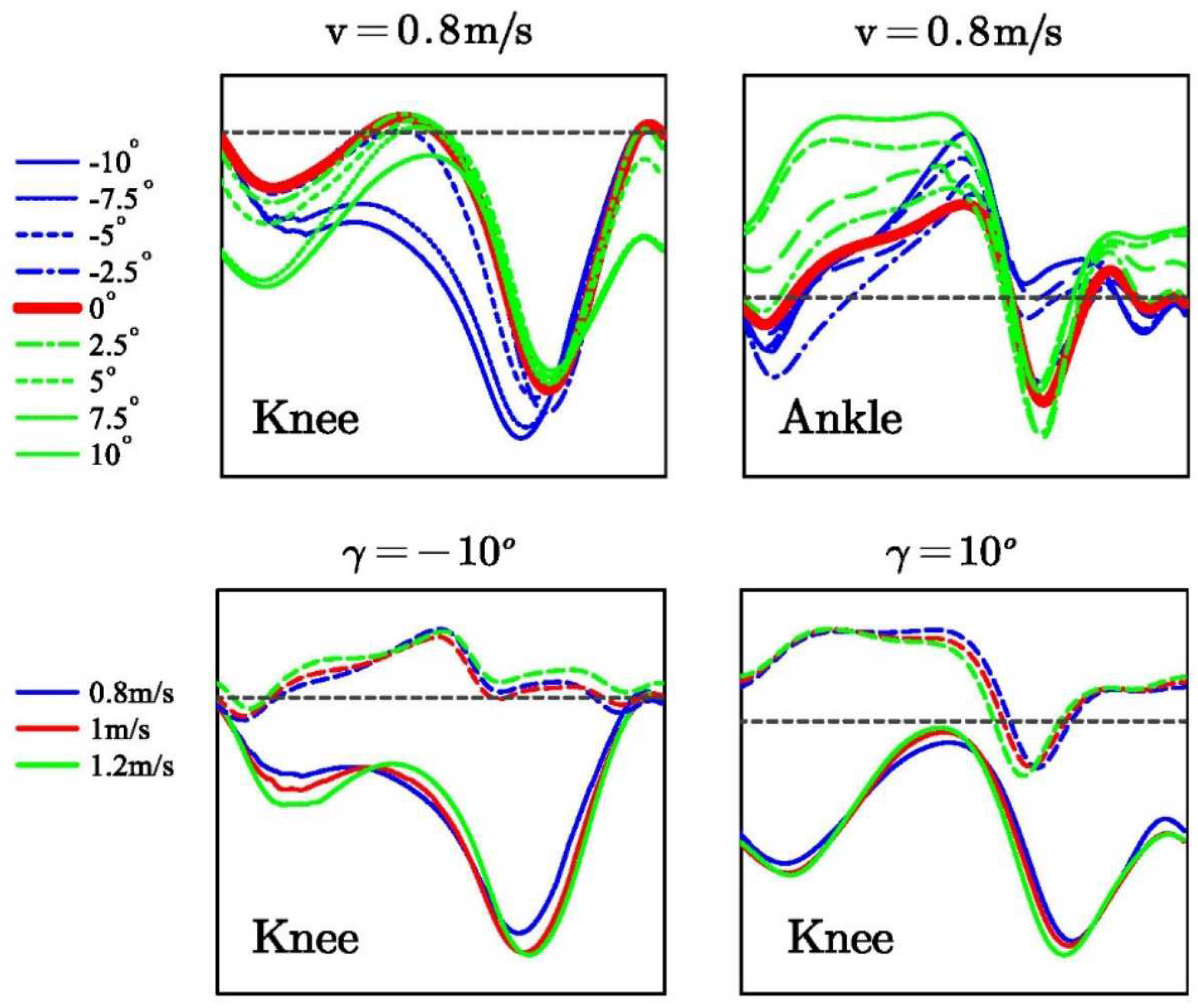
This section describes the adaptive kinematic estimation method. Figure 2 shows knee and ankle angles under varying slopes and constant speed, and the knee angle at different speeds with slopes of −10° and 10°.

When the task variables change, the joint angle also changes accordingly. As the walking speed increases, the maximum swing angle of the knee and ankle joints increases, allowing for a larger stride length in the same amount of time. This shortens the duration of the support period and increases the proportion of the swing period in the gait cycle. When walking on a slope, the knee and ankle joint angles undergo a larger deformation compared to walking on flat ground. At the end of the support phase, the ankle joint transitions from dorsiflexion to plantar flexion when walking uphill. This helps the body overcome gravity and move forward and upward, and results in an increase in the percentage of knee joint flexion time and ankle joint plantar flexion time, showing a state of propulsion. Conversely, when walking downhill, the percentage of knee flexion time decreases and the plantar flexion of the ankle joint increases with the increase in the slope angle.

3.1. Kinematic Estimation Problem Description

In our previous work, we used the Gaussian process (GP) to fit a single-motion trajectory [27]. However, we observed that adaptability to speed and slope was weak. When the walking speed changes, the motion trajectory also changes, and, for different users, the joint kinematics have personalized characteristics that cannot be adjusted accordingly. We also found that the GP curve-fitting method has some disadvantages, such as high computational complexity, which increases with the amount of data and requires a lot of computational resources. Additionally, the choices of kernel functions and hyperparameters affect the fitting effect, which requires a lot of experience and debugging. Furthermore, a large amount of sample data is required, which is not feasible for experiments involving human subjects. Therefore, we developed an adaptive kinematic trajectory estimation algorithm for speed and slope that can be used for subsequent personalized adjustment.

The function for the kinematic modeling of a joint with velocity and slope adaptation is expressed as the following function of the angle of the knee and ankle, with respect to the velocity variable $v$, slope variable $\gamma$, and phase variable $\phi$:

$${\theta }_k^d=q_k\left(\phi ,v,\gamma \right)$$

(8)

$${\theta }_a^d=q_a\left(\phi ,v,\gamma \right)$$

(9)

where $q_k$ and $q_a$ are the function relationships between the knee and ankle joint angles and the phase variable $\phi$. ${\theta }_k^d$ and ${\theta }_a^d$ represent the expected prosthetic joint angles calculated by the gait kinematic model. A unified expression of ${\theta }^d=q\left(\phi ,v,\gamma \right)$ is used in the following section.

A method based on task function weights was proposed in [10], and the gait model was modeled as a basis function with $\phi$ as a variable, and a task function with $v$ and $\gamma$ as variables. Although changes in velocity and slope will lead to changes in kinematic trajectory, there is a basic trajectory shape; the basis function represents the invariant part of the trajectory, while the changes caused by the changes in velocity and slope are reflected in the task function. Thus, the angle expression is as follows:

$$q\left(\phi ,v,\gamma \right)={\displaystyle \sum }_{k=1}^N{b}_k\left(\phi \right)c_k\left(v,\gamma \right)$$

(10)

where $b_k$ is an F-order Fourier series with $\phi$, $c_k\left(v,\gamma \right)$ is a task function with task variables $v$ and $\gamma$, and $n$ is the number of basis functions. We set $F=10$ when $k=1$. When $k\in \left\{2,3,4\right\}$, the slope variable is 0 and the basis function is weighted by the velocity variable. When $k\in \left\{5,6,7,8\right\}$, slope variables are used to weigh the basis function. It can be seen that if $N=8$, the unknown parameters of each basis function are $2F+1=21$, and the total number of unknown parameters in the model is $N\left(2F+1\right)=168$. Due to the large data volume and high computational difficulty, the decipherability of parameters is not exact, and there are certain difficulties in the subsequent adjustment of the model.

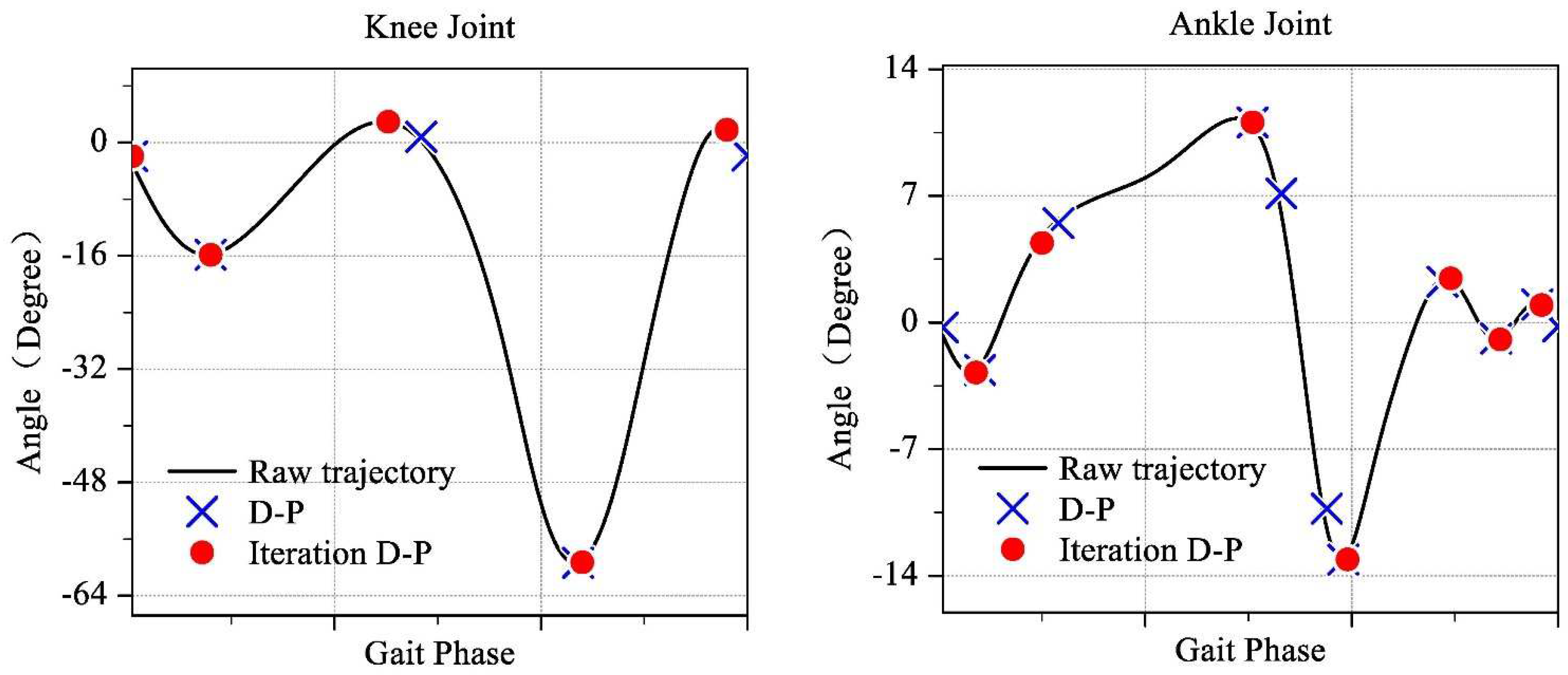
3.2. Key Point Extraction Based on D-P Iteration

Key points can summarize the basic shape of the kinematic curve and affect the trend of the curve. Although the positions of the key points may vary with factors such as individuals’ height and weight, the curves follow a general pattern, with the key points changing within a certain range. Initially, the key point positions of the average gait model are determined, and personalized methods can be subsequently employed for further optimization [27]. The core idea of extracting feature points is to reduce the number of nodes with the premise of maintaining the curve shape characteristics as much as possible. At present, the methods for extracting feature points include vertical distance, slope, angle, etc. The Douglas–Peucker (D-P) extraction algorithm is a commonly used method based on the vertical distance method. The idea is to set the threshold in advance, and then compare the vertical distance of the line from the point on the curve to the first and end points of the curve with the size of the given threshold.

Obviously, the accuracy of the D-P algorithm is related to the chosen threshold. The larger the threshold, the greater the degree of simplification and the fewer key points. On the contrary, the lower the degree of simplification, the more key points, and a curve that is closer to the full shape. The algorithm is prone to the loss of some important feature points when the curvature is large, and to the retention of non-feature points when the bending horizontal distance is small. Therefore, an improved iterative D-P key point extraction method is proposed in this section, which can adaptively extract the global key points of the curve.

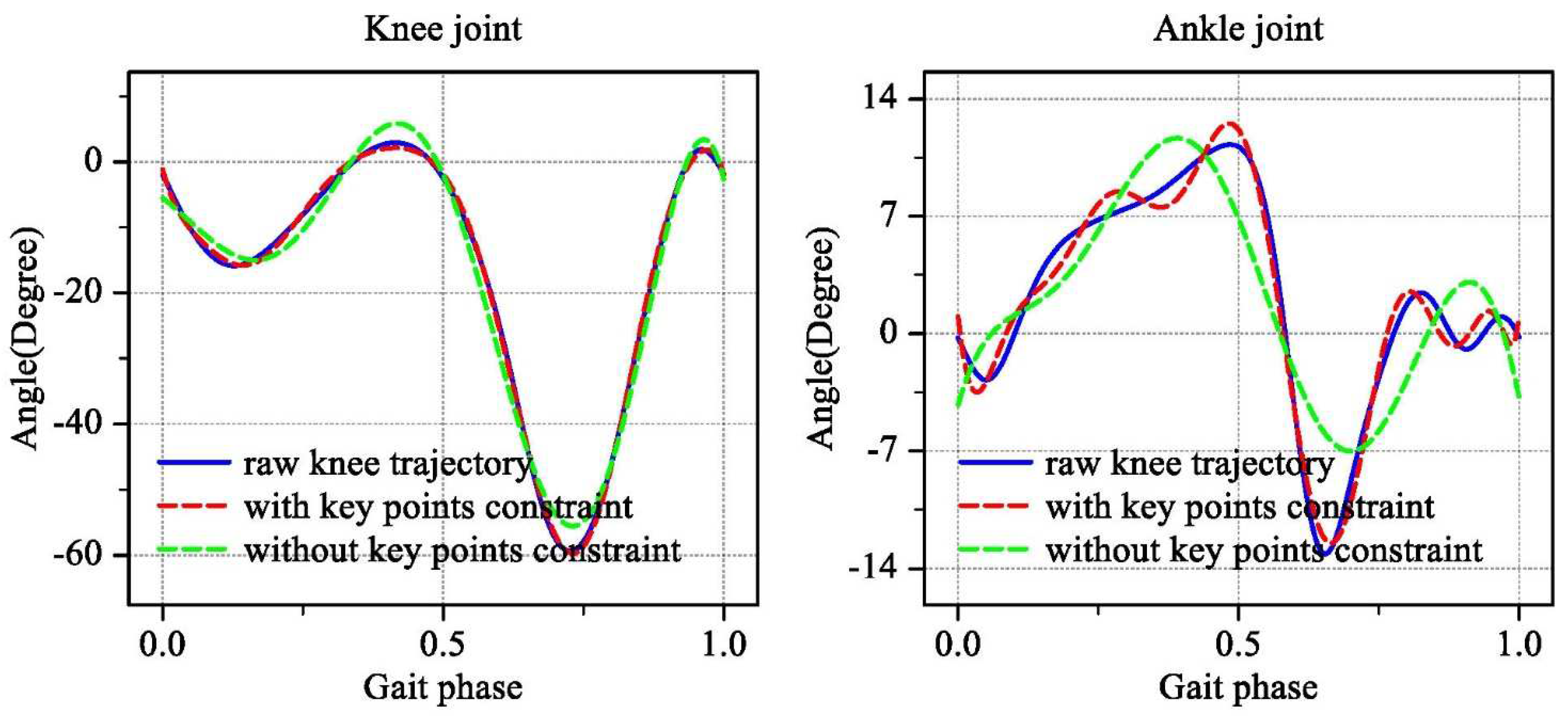
3.3. Invariant Basis Function Estimation Considering Key Points Constraints

The basis function is defined as the gait trajectory with $\phi$ under a speed of 1 m/s and a slope of 0, expressed as follows:

$$q^0=q\left(\phi ,1,0\right)=b\left(\phi \right)$$

(11)

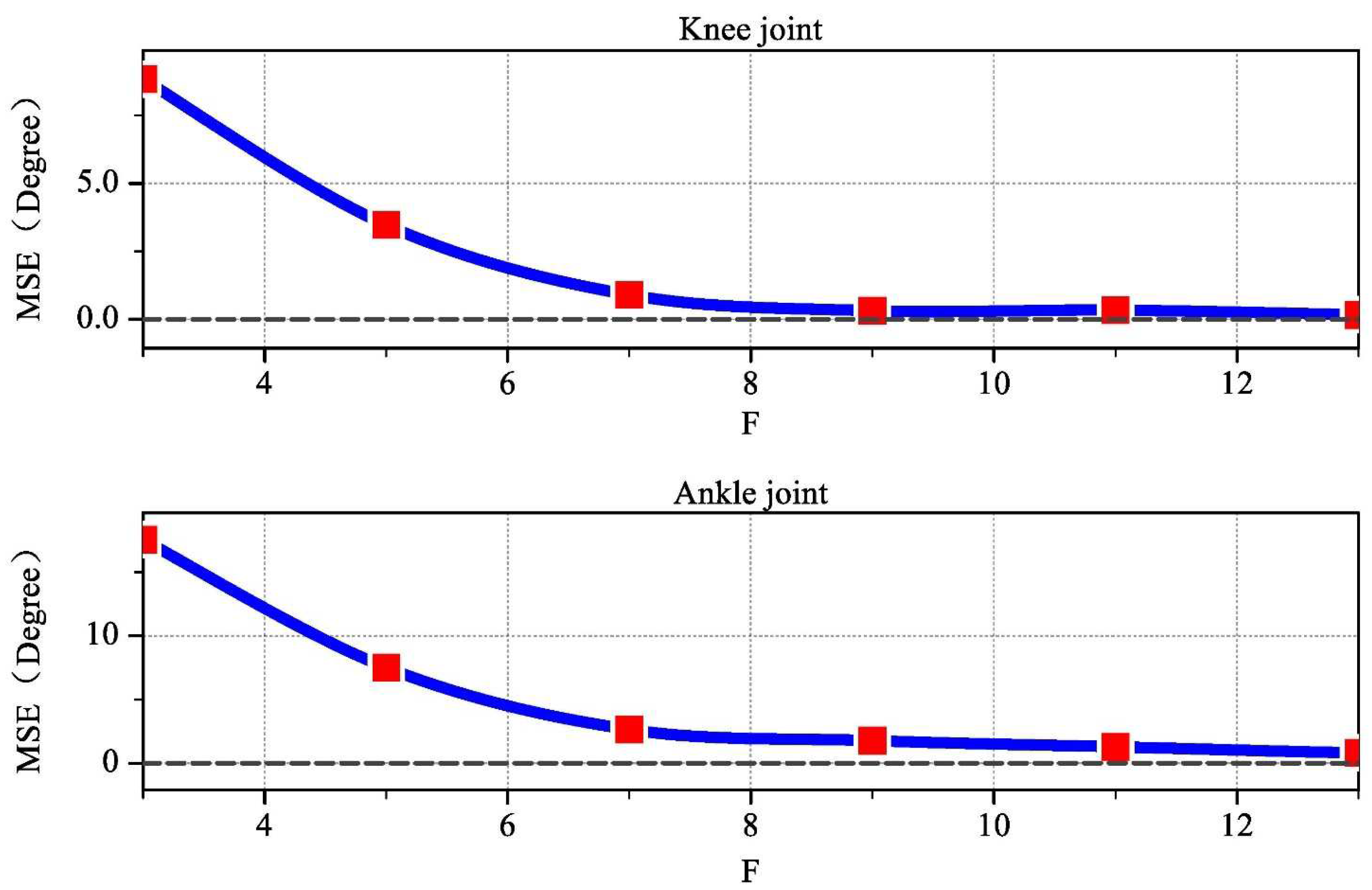
The invariant basis function is fitted by Fourier series, whose expression is as follows:

$$b\left(\phi \right)=a_0+{\displaystyle \sum }_{i=1}^F\left(a_i\sin \left(i\phi \right)+b_i\cos \left(i\phi \right)\right)$$

(12)

where the coefficient matrix ${\left[a_0,a_1,\cdots ,a_F,b_1,b_2,\cdots ,b_F\right]}^T\in {ℝ}^{\left(2F+1\right)\times 1}$ is the order of the Fourier series. Generally, the larger the $F$ is, the better the fitting effect of the specified points is, but it is more likely to cause overfitting.

The first goal of fitting is to fit all data points; on the other hand, the accuracy of fitting key points should be ensured as much as possible. Therefore, the convex optimization method is used to estimate the Fourier coefficient matrix. The form of convex optimization is as follows:

$$\begin{gathered} \underset{ϵ,{ϵ}_k}{\mathrm{minimize}} \xi {ϵ}_k+ϵ \\ subject to-ϵSE\left(q^0\right)\le {\widehat{q}}_i^0-q_i^0\le ϵSE\left(q^0\right) \\ \parallel {\widehat{K}}_j-K_j\parallel \le {ϵ}_K \\ \forall i=1,2,\cdots ,150 \\ \forall j=1,2,\cdots ,l_K \end{gathered}$$

where $q_i^0$ is the $ith$ sampling point of the original trajectory, ${\widehat{q}}_i^0$ is the estimated result, and $SE$ is the standard error of the original data. Similarly, $K_j$ is the jth key point, and ${\widehat{K}}_j$ is the key point position of the estimated result. $ϵ$ and ${ϵ}_K$ are the optimization targets indicating that the estimated error is as small as possible, and $l_K$ is the number of key points of the current curve. $ϵ$ and ${ϵ}_K$ are weighted by the proportional coefficient $\xi$ to create a bias between the curve global domain and the key point domain.

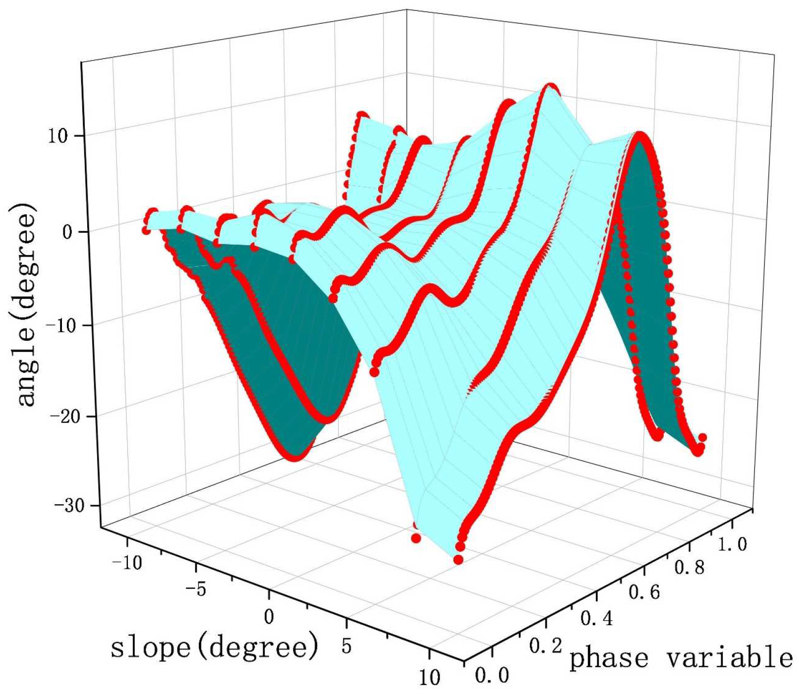
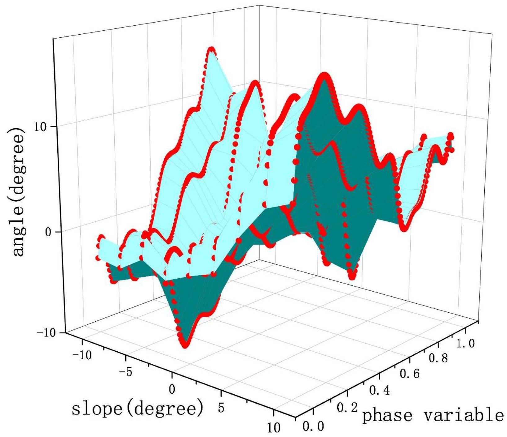
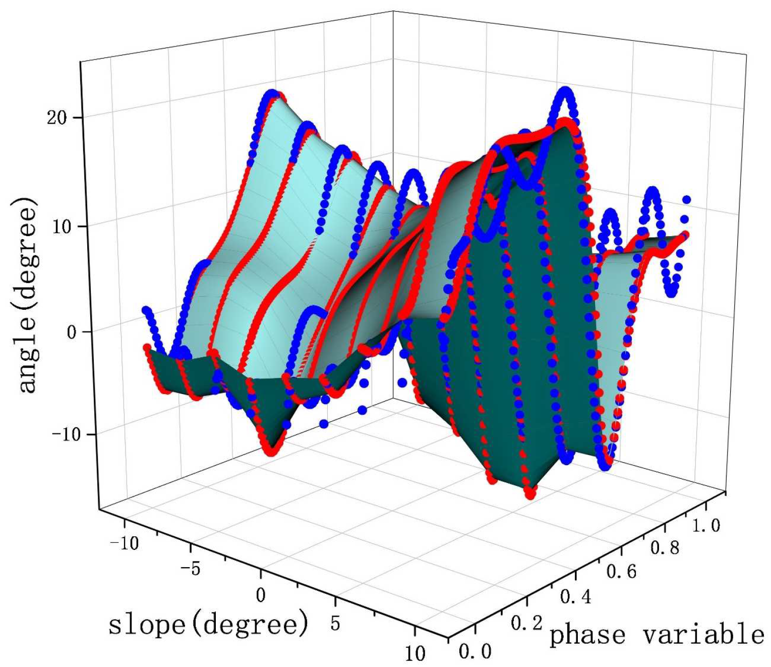
3.4. Adaptive Task Function Estimation Based on RBF Neural Network

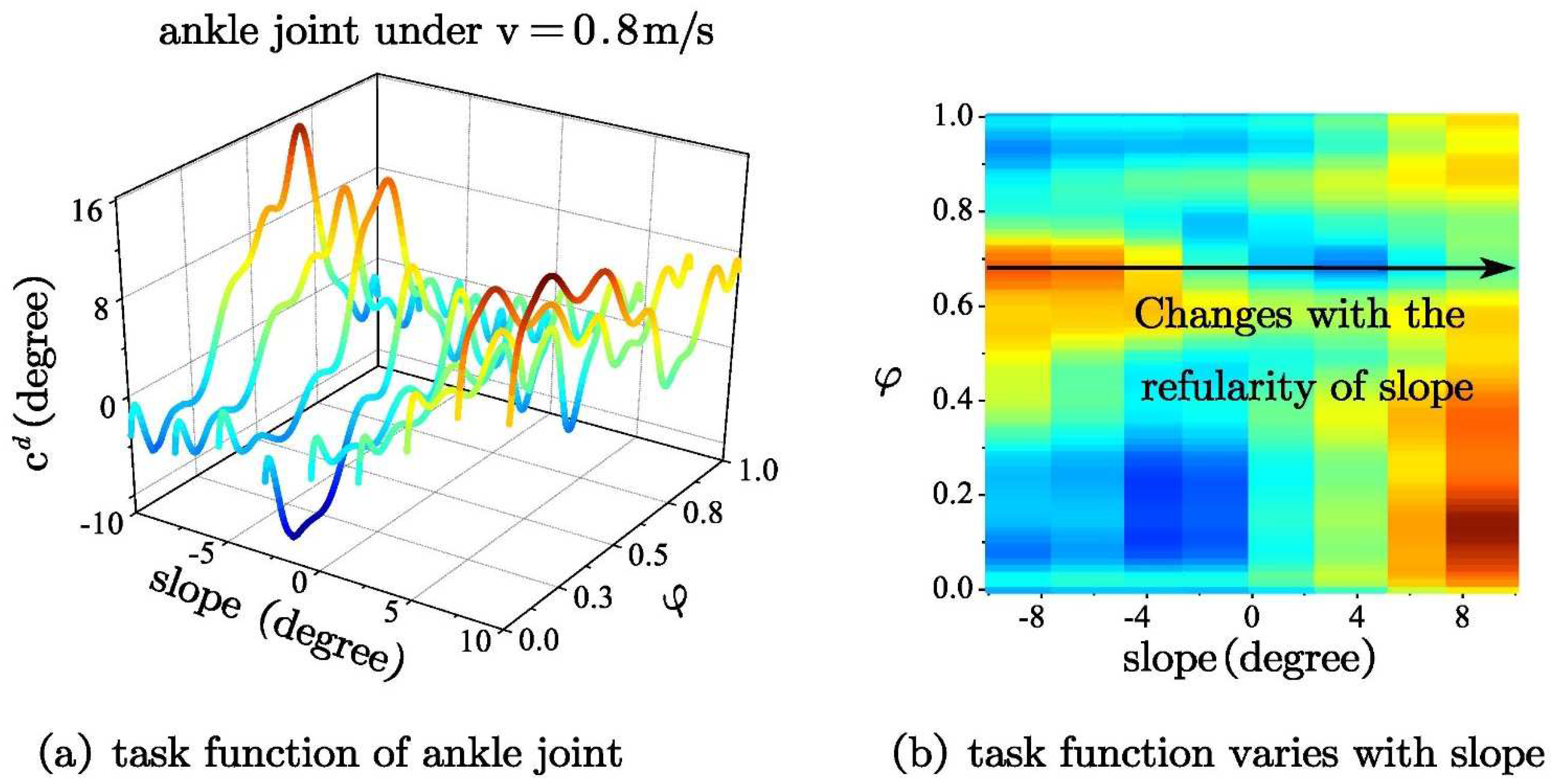
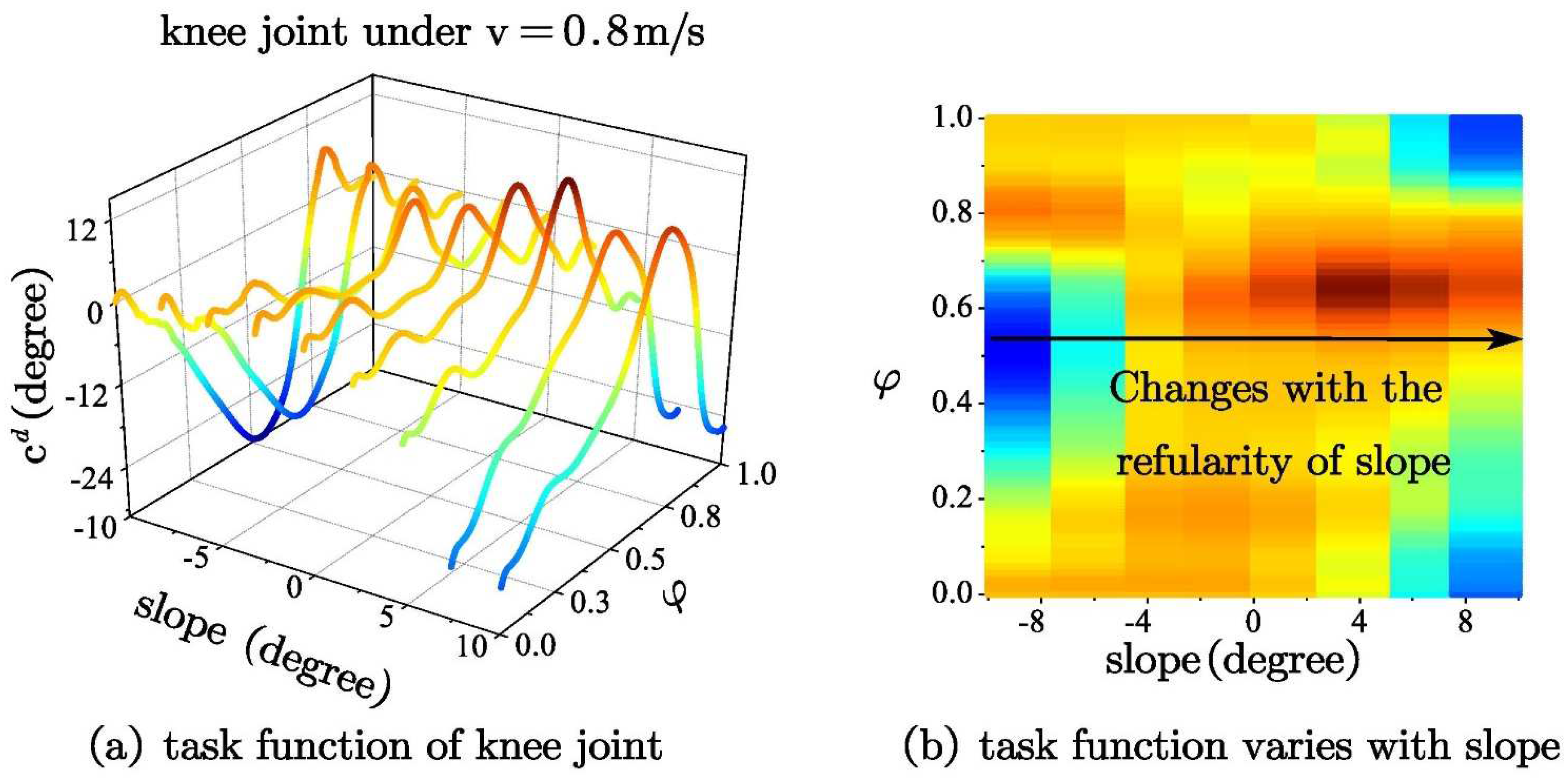
The purpose of the task function is to enable the kinematic model to adaptively generate the expected motion trajectory of the joint according to the current task, so as to provide more reasonable guidance for the prosthetic controller. The task function represents the function of the task vector $\chi =\left(v,\gamma \right)$, where $v$ is the forward velocity of the subject. The task vector matrix $\chi$ can be expanded according to the specific requirements to cope with more changes in walking conditions, such as standing or sitting. The desired task function can be calculated by the following:

$$c^d\left(\phi ,\chi \right)=q^d\left(\phi ,\chi \right)-b\left(\phi \right)$$

(13)

where $q^d\left(\phi ,\chi \right)$ is the expected trajectory provided by the data set. As shown in Figure 3 and Figure 4, the obtained surface of the task function changing with slope at the three speeds shows that the value of $c^d$ is correlated with the change in slope in each phase variable dimension and presents a nonlinear change trend.

In this study, a radial basis function (RBF) neural network was used to fit the task function. RBF is a kind of feedback neural network with good performance, which is suitable for solving nonlinear problems. The basic idea is to transform the input vector by introducing the radial basis function as the activation function of the hidden layer neuron, and transform the low-dimensional input data into a high-dimensional space, so that the neural network can better approximate the nonlinear function. The input vector is $X={\left[x_1,x_2,\cdots ,x_n\right]}^T$, and the radial basis vector is $H={\left[h_1,h_2,\cdots ,h_m\right]}^T$, where $h_j$ is the following Gaussian basis function:

$$h_j=\exp \left(-\frac{\parallel X-c_j\parallel }{2b_j^2},j=1,2,\cdots ,m\right)$$

(14)

where $c_j$ is the center vector of the jth node of the network. When the base width vector of the network is set to $B={\left[b_1,b_2,\cdots ,b_m\right]}^T$, $b_j$ is the base width function of node $j$. The weight vector is $W={\left[{\omega }_1,{\omega }_2,\cdots ,{\omega }_m\right]}^T$. The resulting output is as follows:

$$y_m\left(t\right)={\omega }_1{h}_1+{\omega }_2{h}_2+\cdots +{\omega }_m{h}_m$$

(15)

According to the gradient descent method, the iterative algorithm of the output weight, node center, and node base width parameters are as follows:

$${\omega }_j\left(t\right)={\omega }_j\left(t-1\right)+\eta \left(y\left(t\right)-y_m\left(t\right)\right)h_j+\alpha \left({\omega }_j\left(t-1\right)-{\omega }_j\left(t-2\right)\right)$$

(16)

$$\Delta b_j=\left(y\left(t\right)-y_m\left(t\right)\right){\omega }_j{h}_j\frac{\parallel X-C_j{\parallel }^2}{b_j^3}$$

(17)

$$b_j\left(t\right)=b_j\left(t-1\right)+\eta \Delta b_j+\alpha \left(b_j\left(t-1\right)-b_j\left(t-2\right)\right)$$

(18)

$$\Delta c_{ji}=\left(y\left(t\right)-y_m\left(t\right)\right){\omega }_j\frac{x_i-c_{ji}}{2b_j^2}$$

(19)

$$c_{ji}\left(t\right)=c_{ji}\left(t-1\right)+\eta \Delta c_{ji}+\alpha \left(c_{ji}\left(t-1\right)-c_{ji}\left(t-2\right)\right)$$

(20)

where $\eta$ is the learning rate and $\alpha$ is the momentum factor.

4. Experiments and Results

4.1. Key Point Extraction

The key points were extracted through the compression of the knee and ankle trajectories of an experimenter. Two different methods, the traditional D-P algorithm and the improved iterative D-P key point extraction algorithm, were used for processing. As shown in Figure 5, appropriate thresholds were utilized for the traditional D-P algorithm. The iterative D-P method extracted 5 and 7 key points, respectively, from the knee and ankle joint trajectories; the numbers of the key points extracted by the traditional D-P method were 5 and 11, and the improved method showed a better compression rate.

In terms of key point location selection, the iterative D-P method was effective at selecting the curvature mutation point and shape inflection point of the curve, whereas the traditional D-P method could not guarantee that the selected key point was at the deformation point of the curve due to limitations in the method. The improved method showed better results in terms of compression rate and key point location.

The final results are shown in

Table 1. Key point positions of knee joint.

Knee	${\mathit{K}}_{\mathit{k}1}$	${\mathit{K}}_{\mathit{k}2}$	${\mathit{K}}_{\mathit{k}3}$	${\mathit{K}}_{\mathit{k}4}$	${\mathit{K}}_{\mathit{k}5}$
$\mathit{\phi }$	0.007	0.133	0.420	0.733	0.967
Degree	−1.924	−15.856	2.946	−59.283	1.803

and

Table 2. Key point positions of ankle joint.

Ankle	${\mathit{K}}_{\mathit{a}1}$	${\mathit{K}}_{\mathit{a}2}$	${\mathit{K}}_{\mathit{a}3}$	${\mathit{K}}_{\mathit{a}4}$	${\mathit{K}}_{\mathit{a}5}$	${\mathit{K}}_{\mathit{a}6}$	${\mathit{K}}_{\mathit{a}7}$
$\mathit{\phi }$	0.060	0.167	0.507	0.660	0.827	0.907	0.973
Degree	−2.758	4.403	11.071	−13.086	2.444	−0.937	0.969

. The key point set of the knee joint is $K_k=\left[K_{k1},K_{k2},\cdots ,K_{k5}\right]$ and of the ankle joint is $K_a=\left[K_{a1},K_{a2},\cdots ,K_{a7}\right]$.

4.2. Basis Function Estimation

The basis function of the kinematic trajectories of the knee and ankle joints were fitted, and the experimental results were obtained. The experimental results are displayed in Figure 6. By introducing the constraints of key point positions, the fitted curve could achieve better accuracy at these critical points. This leads to gait kinematics that more closely resemble those of healthy individuals. While the transition segment between the key points is less demanding in terms of accuracy for practical purposes, the key points themselves are crucial in determining gait differences. They impact the sequence of each gait event and characteristics such as step length.

In addition, it is necessary to determine the order $F$ of Fourier series in basis function fitting. Figure 7 shows the influence of different orders on experimental results, and uses Mean Square Error ($MSE$) to quantify the accuracy of fitting as follows:

$$MSE=\frac{1}{n}{\displaystyle \sum }_{i=1}^n{\left(q^0-{\widehat{q}}^0\right)}^2$$

(21)

where $n$ is the sample number. The MSE between the curve to be fitted and the fitting results decreases with an increase in $F$ at different orders. When $F$ increases to a certain amount, the deceleration in milliseconds tends to be gradual and even leads to overfitting. Therefore, the order of knee joint fitting $F_K$ was set to 9, and that of ankle joint fitting was set to 13. The MSEs of the invariant basis function were 0.338 degrees and 0.809 degrees, respectively.

4.3. Task Function Estimation

This study used the data set provided in [28], which greatly supported our research. This data set contained three-dimensional biomechanics and wearable sensor data under three speeds and nine ground slopes. The speeds used were 0.8, 1.0, 1.2 m/s, and the slopes varied linearly from −10 to 10 degrees, with a total of 27 groups of experimental data used. The 27 groups of gait data were taken as the training set. The input vector

$$\begin{gathered} X={\left[{\chi }_1^T,{\chi }_2^T,\cdots ,{\chi }_{27}^T\right]}^T \\ \hspace{1em}\hspace{1em}\hspace{1em}\hspace{1em}\hspace{1em}\hspace{1em}\hspace{1em}\hspace{1em}={\left[\begin{array}{c}{v}_1,\cdots ,v_1,v_2,\cdots ,v_2,v_3,\cdots ,v_3\\ {\gamma }_1,\cdots ,{\gamma }_9,{\gamma }_1,\cdots ,{\gamma }_9,{\gamma }_1,\cdots ,{\gamma }_9\end{array}\right]}^T \end{gathered}$$

(22)

included combinations of the speeds and slopes, where ${\chi }_i$ was the ith combination of the task variables. The output vectors were set as follows:

$$Y_k=\left[q_k^d\left({\chi }_1\right),\cdots ,q_k^d\left({\chi }_{27}\right)\right]$$

(23)

$$Y_a=\left[q_a^d\left({\chi }_1\right),\cdots ,q_a^d\left({\chi }_{27}\right)\right]$$

(24)

In the experiment, the RBF neural network was a three-layer structure, and the hidden layer node was set to 10. Figure 8 and Figure 9 represent the results of task function estimation. The curve surface shows the continuous estimation results, and the red dots provide the gait data set, which is the desired target. It can be seen that the estimated results fit the expected value of the database and achieve good accuracy.

The estimation results of the total joint kinematics are shown in Figure 10 and Figure 11. The curve surface shows the continuous estimation results, the red dots give the gait data set, and the surface fits close to the desired gait trajectories. The blue dots are the estimation results obtained by using the method outlined in [19]; it is clear that the method shows larger errors than when using the method in this article. Figure 12 takes the knee joint estimation errors as examples to show the detailed MSE of the two methods. The proposed method greatly improved the accuracy of estimation.

5. Discussion

5.1. The Advantages of the Kinematic Estimation Method

Upon theoretical analysis and experimental verification, this study’s proposed kinematic estimation method based on the key points has the following benefits:

(1) This method is designed to obtain a global continuous kinematic model with limited gait database data. Human experimental data are limited, making it impossible to obtain gait data for arbitrary continuous speeds and slopes. This method builds a kinematic model using the limited data and estimates the unknown gait between experimental data based on the regular differences caused by speeds and slopes. Gait kinematics are divided into two parts: the invariant basis function and task function. Fitting and estimation are carried out, respectively, to reduce the complexity of the model and the difficulty of the calculation.

(2) A new method has been proposed to estimate the key points of the gait model. The improved iterative D-P algorithm automatically locates these key points and introduces the constraint of the key points into the basis function solution. The use of the key points in the basis function has several advantages. Firstly, it ensures that the key points, which determine gait characteristics, are retained to ensure that the same action is performed with the reference gait in the key gait phases. This helps to improve walking comfort and stability. Secondly, individualization is usually a difficult problem to solve in prosthetic control. However, the gait differences of different people can be reflected by the key points, which makes it an effective and concise method to adjust the basis function through the key points.

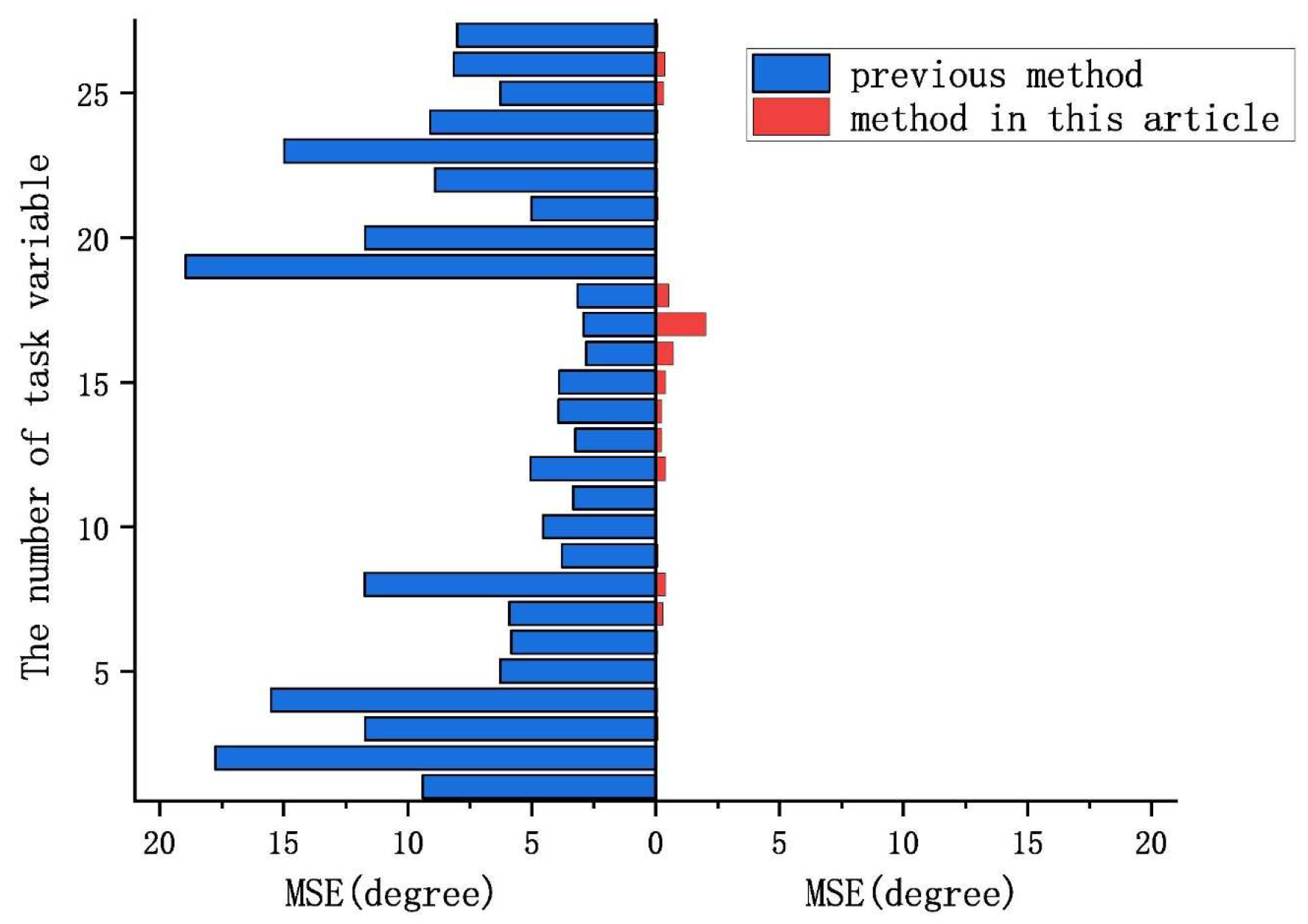
(3) The RBF neural network is used to estimate the task function, adaptively adjust the network model, and build an adaptive estimation method for speeds and slopes with high estimation accuracy.

5.2. Future Works

Our research method requires further work to be carried out. The first step is to study the individual optimization method based on the invariant basis function using the key points. In our previous work, an individual control method based on gait trajectory key points was raised [27]. The next step is to build a regression model based on the wearer’s individual characteristics such as their height and weight. The individual model will be updated through the active feedback of the user. The kinematic model will then be used to provide a trajectory reference for the underlying control of the prosthetic limb. The dynamic control method of the prosthesis will be studied using compliant control methods such as impedance control. Finally, the performance of the prosthetic prototype and control methods will be verified by conducting experiments on amputee patients.

6. Conclusions

A new method for estimating the kinematics of the knee and ankle joints was proposed in this study. This method uses the upper control layer of a dynamic lower limb prosthesis to create a kinematic model that adapts to velocity and slope. The model is composed of two parts: an invariant basis function based on key points, and an adaptive task function based on an RBF neural network. Together, they accurately estimate joint movements based on the current phase and task variables. This method also serves as a foundation for further research into personalized optimization and compliant control methods.

References

1. Wen, Y.; Si, J.; Gao, X.; Huang, S.; Huang, H.H. A New Powered Lower Limb Prosthesis Control Framework Based on Adaptive Dynamic Programming. IEEE Trans. Neural Netw. Learn. Syst. 2017, 28, 2215–2220. [Google Scholar] [CrossRef] [PubMed]
2. Lv, G.; Gregg, R.D. Underactuated Potential Energy Shaping with Contact Constraints: Application to a Powered Knee-Ankle Orthosis. IEEE Trans. Control Syst. Technol. 2018, 26, 181–193. [Google Scholar] [CrossRef] [PubMed]
3. Nitish, T.; Hartmut, G. Toward balance recovery with leg prostheses using neuromuscular model control. IEEE Trans. Biomed. Eng. 2016, 63, 904–913. [Google Scholar]
4. Todorov, E.; Jordan, M. Optimal feedback control as a theory of motor coordination. Nat. Neurosci. 2002, 5, 1226–1235. [Google Scholar] [CrossRef] [PubMed]
5. Chehab, E.; Andriacchi, T.; Favre, J. Speed, age, sex, and body mass index provide a rigorous basis for comparing the kinematic and kinetic profiles of the lower extremity during walking. J. Biomech. 2017, 58, 11–20. [Google Scholar] [CrossRef] [PubMed]
6. Lelas, J.L.; Merriman, G.J.; Riley, P.O.; Kerrigan, D.C. Predicting peak kinematic and kinetic parameters from gait speed. Gait Posture 2003, 17, 106–112. [Google Scholar] [CrossRef] [PubMed]
7. Koopmana, B.; Asseldonka, E.H.F.v.; der Kooija, H.v. Speed-dependent reference joint trajectory generation for robotic gait support. J. Biomech. 2014, 47, 1447. [Google Scholar] [CrossRef] [PubMed]
8. Tucker, M.R.; Olivier, J.; Pagel, A.; Bleuler, H.; Bouri, M.; Lambercy, O.; del R Millan, J.; Riener, R.; Vallery, H.; Gassert, R. Control strategies for active lower extremity prosthetics and orthotics: A review. J. NeuroEng. Rehabil. 2015, 12, 1. [Google Scholar] [CrossRef] [PubMed]
9. Embry, K.R.; Villarreal, D.J.; Gregg, R.D. A unified parameterization of human gait across ambulation modes. In Proceedings of the Annual International Conference of the IEEE Engineering in Medicine and Biology Society, Lake Buena Vista, FL, USA, 16–20 August 2016; pp. 2179–2183. [Google Scholar]
10. Embry, K.R.; Villarreal, D.J.; Macaluso, R.L.; Gregg, R.D. Modeling the Kinematics of Human Locomotion Over Continuously Varying Speeds and Inclines. IEEE Trans. Neural Syst. Rehabil. Eng. 2018, 26, 2342–2350. [Google Scholar] [CrossRef]
11. Best, T.K.; Embry, K.R.; Rouse, E.J.; Gregg, R.D. Phase-Variable Control of a Powered Knee-Ankle Prosthesis over Continuously Varying Speeds and Inclines. In Proceedings of the 2021 IEEE/RSJ International Conference on Intelligent Robots and Systems (IROS), Prague, Czech Republic, 27 September–1 October 2021. [Google Scholar]
12. Asbeck, A.T.; Dyer, R.J.; Larusson, A.F.; Walsh, C.J. Biologically-inspired Soft Exosuit. In Proceedings of the 2013 IEEE 13th International Conference on Rehabilitation Robotics (ICORR), Seattle, WA, USA, 24–26 June 2013. [Google Scholar]
13. Andersen, J.; Sinkjaer, T. Mobile ankle and knee perturbator. IEEE Trans. Biomed. Eng. 2003, 50, 1208–1211. [Google Scholar] [CrossRef]
14. Sulzer, J.S.; Gordon, K.E.; Hornby, T.G.; Peshkin, M.A.; Patton, J.L. Adaptation to knee flexion torque during gait. In Proceedings of the 2009 IEEE International Conference on Rehabilitation Robotics, Kyoto, Japan, 23–26 June 2009. [Google Scholar]
15. Ijspeert, A.J. School of Computer and Communication Sciences and Ecole Polytechnique Federale de Lausanne. Central pattern generators for locomotion control in animals and robots: A review. Neural Netw. 2008, 21, 642–653. [Google Scholar] [CrossRef] [PubMed]
16. Colgate, J.E.; Hogan, N. Robust control of dynamically interacting systems. Int. J. Control. 1988, 48, 65–88. [Google Scholar] [CrossRef]
17. Shultz, A.; Goldfarb, M. A unified controller for walking on even and uneven terrain with a powered ankle prosthesis. IEEE Trans. Neural Syst. Rehabil. Eng. 2018, 26, 788–797. [Google Scholar] [CrossRef] [PubMed]
18. Torrealba, R.; Cappelletto, J.; Fermín, L.; Fernandez-Lopez, G.; Grieco, J.C. Cybernetic knee prosthesis: Application of an adaptive central pattern generator. Kybernetes 2012, 41, 192–205. [Google Scholar] [CrossRef]
19. Ledoux, E.; Goldfarb, M. Control and Evaluation of a Powered Transfemoral Prosthesis for Stair Ascent. IEEE Trans. Neural Syst. Rehabil. Eng. 2017, 25, 917–924. [Google Scholar] [CrossRef] [PubMed]
20. Culver, S.; Bartlett, H.; Shultz, A.; Goldfarb, M. A Stair Ascent and Descent Controller for a Powered Ankle Prosthesis. IEEE Trans. Neural Syst. Rehabil. Eng. 2018, 26, 993–1002. [Google Scholar] [CrossRef]
21. Shultz, A.H.; Lawson, B.E.; Goldfarb, M. Variable cadence walking and ground adaptive standing with a powered ankle prosthesis. IEEE Trans. Neural Syst. Rehabil. Eng. 2016, 24, 495–505. [Google Scholar] [CrossRef] [PubMed]
22. Shultz, A.H.; Lawson, B.E.; Goldfarb, M. Running with a powered knee and ankle prosthesis. IEEE Trans. Neural Syst. Rehabil. Eng. 2015, 23, 403–412. [Google Scholar] [CrossRef]
23. Shultz, A.; Lawson, B.; Goldfarb, M. Walking on uneven terrain with a powered ankle prosthesis: A preliminary assessment. In Proceedings of the 2015 37th Annual International Conference of the IEEE Engineering in Medicine and Biology Society (EMBC), Milano, Italy, 25–29 August 2015. [Google Scholar]
24. Mohammadi, H.; Richter, H. Robust Tracking/lmpedance Control: Application to Prosthetics. In Proceedings of the 2015 American Control Conference (ACC), Chicago, IL, USA, 1–3 July 2015; pp. 2673–2678. [Google Scholar]
25. Lawson, B.E.; Ruhe, B.; Shultz, A.; Goldfarb, M. A powered prosthetic intervention for bilateral transfemoral amputees. IEEE Trans. Biomed. Eng. 2015, 62, 1042–1050. [Google Scholar] [CrossRef]
26. Reznick, E.; Embry, K.; Gregg, R.D. Predicting Individualized Joint Kinematics over a Continuous Range of Slopes and Speeds. In Proceedings of the 2020 8th IEEE RAS/EMBS International Conference for Biomedical Robotics and Biomechatronics (BioRob), New York, NY, USA, 29 November–1 December 2020. [Google Scholar]
27. Sun, L.; Ma, H.; An, H.; Wei, Q. An Individual Prosthesis Control Method with Human Subjective Choices. Biomimetics 2024, 9, 77. [Google Scholar] [CrossRef]
28. Camargo, J.; Ramanathan, A.; Flanagan, W.; Young, A. A comprehensive, open-source dataset of lower limb biomechanics in multiple conditions of stairs, ramps, and level-ground ambulation and transitions. J. Biomech. 2021, 119, 110320. [Google Scholar] [CrossRef] [PubMed]
Figure 1. The intelligent prosthesis prototype being worn by a subject. The sensors include IMU and a foot-pressure sensor. Two motors are located on the knee and ankle joints.
Applsci 14 03063 g001
Figure 2. Knee and ankle angles at constant speed and varying slopes, and the knee angle at different speeds when the slope changes. The grey dashed line represents 0 degrees.
Applsci 14 03063 g002
Figure 3. Knee joint task function under 0.8 m/s. The value changes relative to slope in each phase variable dimension and presents a nonlinear change trend. (a) represents how the task function changes with slope and phase variable. (b) visually illustrates the regular change of the task function with slope.
Applsci 14 03063 g003
Figure 4. Ankle joint task function under 0.8 m/s. The value changes relative to slope in each phase variable dimension and presents a nonlinear change trend. (a) represents how the task function changes with slope and phase variable. (b) visually illustrates the regular change of the task function with slope.
Applsci 14 03063 g004
Figure 5. The results of key point extraction by using iteration D-P method.
Applsci 14 03063 g005
Figure 6. Fitting results of basis function.
Applsci 14 03063 g006
Figure 7. MSE of invariant basis function estimation with different orders. The red dots are the MSEvalues obtained under the corresponding orders, and the blue solid line describes the trend of MSE with the order. The dashed grey line indicates the location where MSEis 0.
Applsci 14 03063 g007
Figure 8. The estimated result of the task function of the knee joint. The blue surface is the final task function model, and the red dashed lines are the fitting data.
Applsci 14 03063 g008
Figure 9. The estimated result of the task function of the ankle joint. The blue surface is the final task function model, and the red dashed lines are the fitting data.
Applsci 14 03063 g009
Figure 10. The estimated result of knee joint kinematics. The blue surface is the final task function model, and the red dashed lines are the fitting data, and the blue dashed lines are the results calculated by the method in [19].
Applsci 14 03063 g010
Figure 11. The estimated result of ankle joint kinematics. The blue surface is the final task function model, and the red dashed lines are the fitting data, and the blue dashed lines are the results calculated by the method in [19].
Applsci 14 03063 g011
Figure 12. MSE of the estimated results by using the two methods.
Applsci 14 03063 g012