
Low-Carbon Logistics Distribution Vehicle Routing Optimization Based on INNC-GA

Abstract
1. Introduction
2. Problem Description and Basic Assumptions
- (1)
- The distribution center’s location is predetermined, with all vehicles originating from and returning to this center upon task completion.
- (2)
- The types of vehicles in the distribution center are indistinguishable.
- (3)
- The requirements of each customer are known, and all are within the maximum load capacity of the vehicle.
- (4)
- It is strictly forbidden to violate the customer’s time window and it is required that the delivery must be completed within the time window.
- (5)
- The weight of the cargo in each vehicle must not exceed its maximum load capacity.
- (6)
- Each customer should be served by a single vehicle, without any overlap.
- (7)
- The vehicles travel at a fixed speed, regardless of factors such as traffic congestion or environmental conditions.
3. Model Construction
3.1. Distance Calculation Method
3.2. Construction of the Model
4. INNC-GA
4.1. INNC
4.2. GA
- (1)
- Chromosome: The genetic makeup of an individual. A population consists of multiple chromosomes.
- (2)
- Bit string: A representation of an individual, similar to a chromosome in natural genetics.
- (3)
- Gene: A specific position within a chromosome that corresponds to a characteristic or variable of the solution.
- (4)
- Individual: A solution represented by a chromosome in a genetic algorithm.
- (5)
- Fitness: A measure of an individual’s performance in solving a problem. It is used to assess the strengths and weaknesses of individuals and aid in selection.
- (6)
- Genotype: The composition of genes on an individual’s chromosome. It serves as the encoded representation of the individual within a genetic algorithm.
- (7)
- Phenotype: The observable trait or characteristic displayed by an individual in the external environment. In genetic algorithms, the phenotype corresponds to the specific solution or characteristic encoded by the genotype.
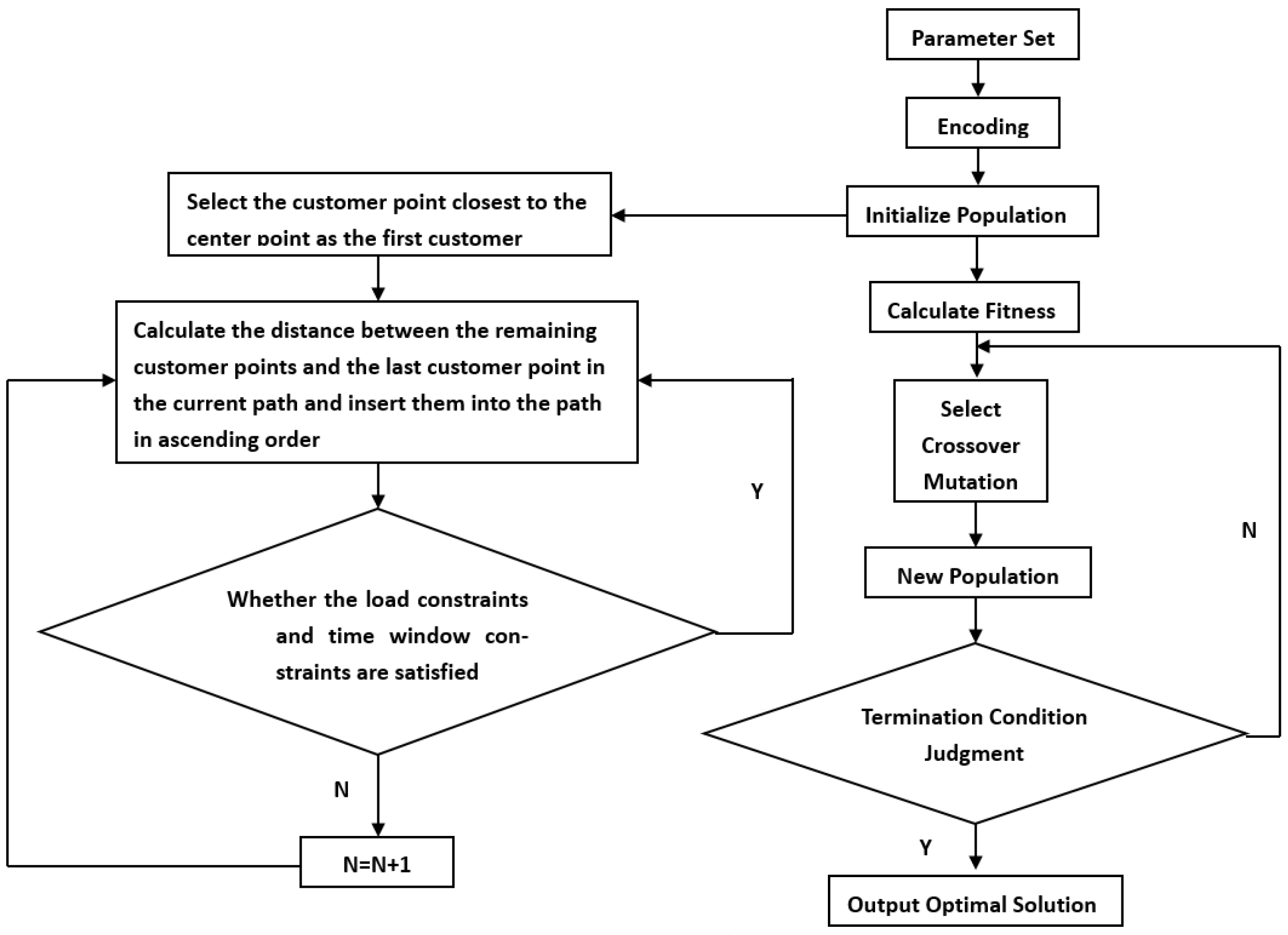
4.3. INNC-GA
- (1)
- Coding
- (2)
- Initialization of the population
- (3)
- Fitness Function
- (4)
- Selection
- (5)
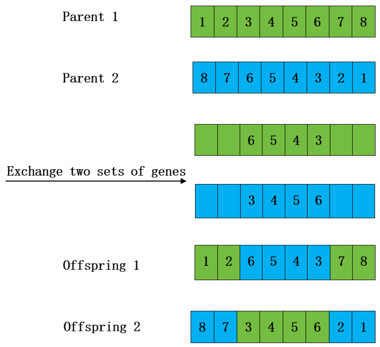
- OX Crossover
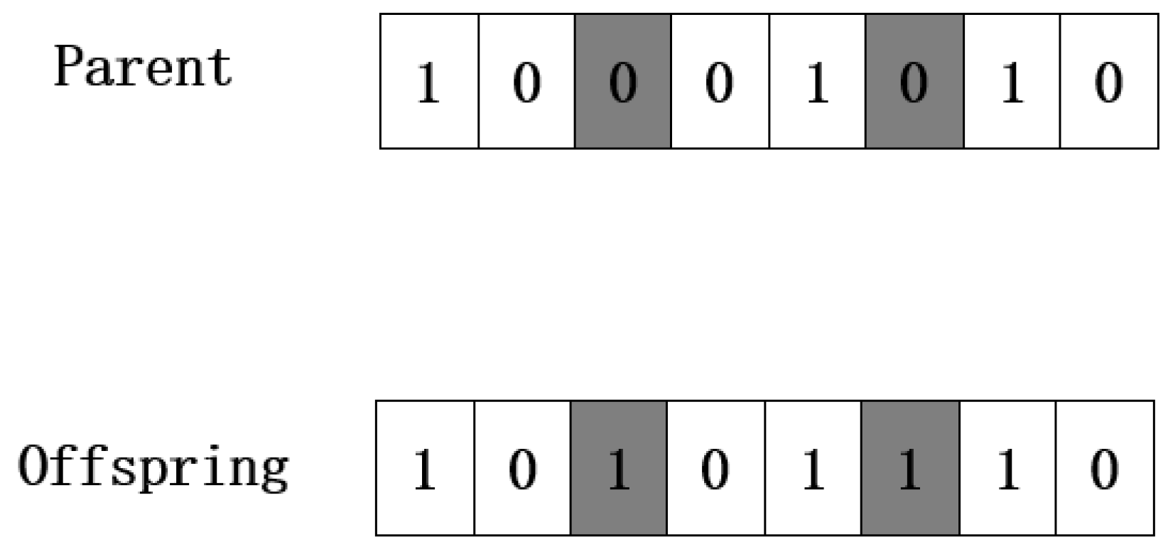
- (6)
- Mutation
5. Comparison and Analysis of Experimental Results
5.1. Experimental Setup
5.2. Effects of the Initial Solution
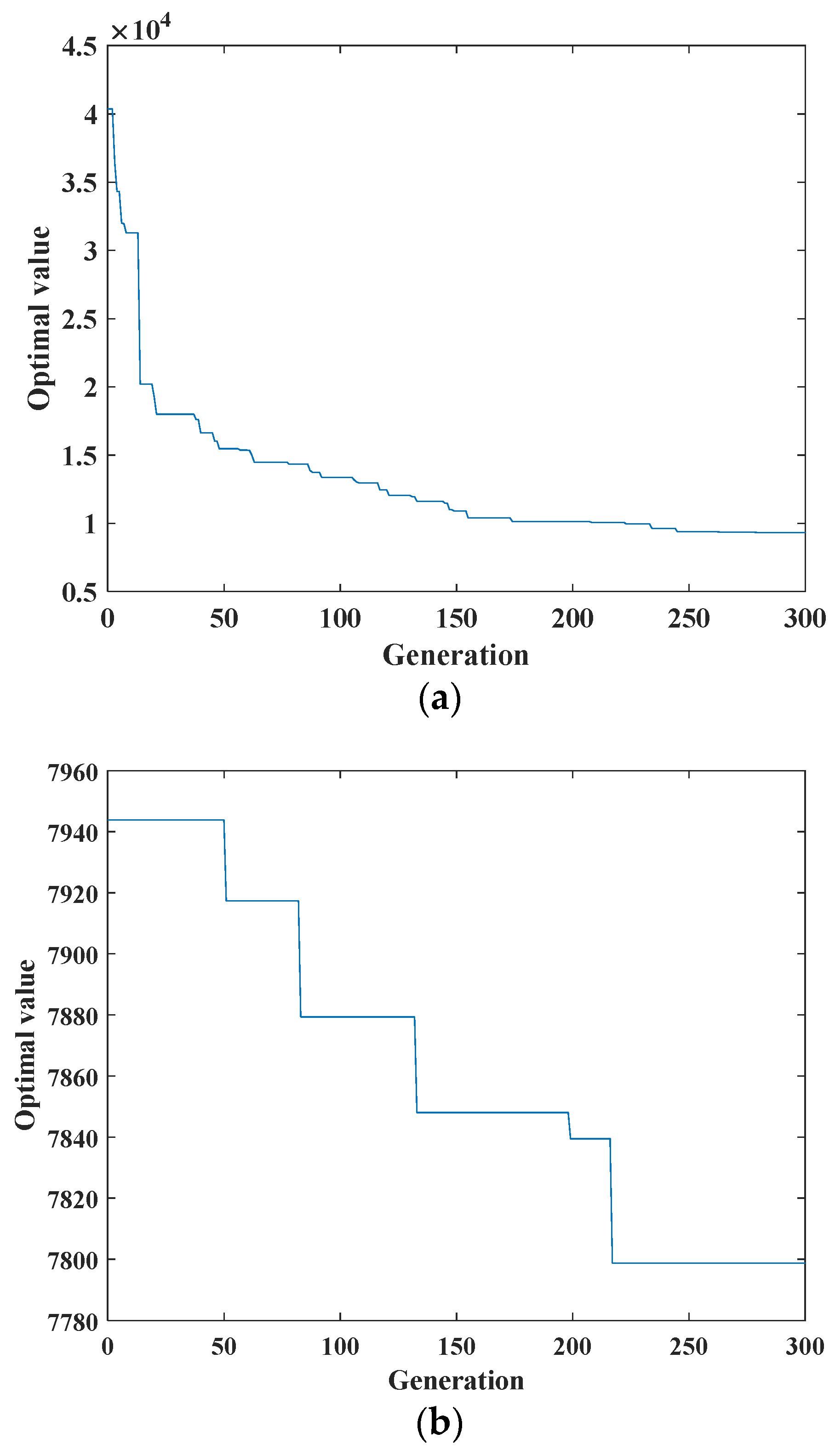
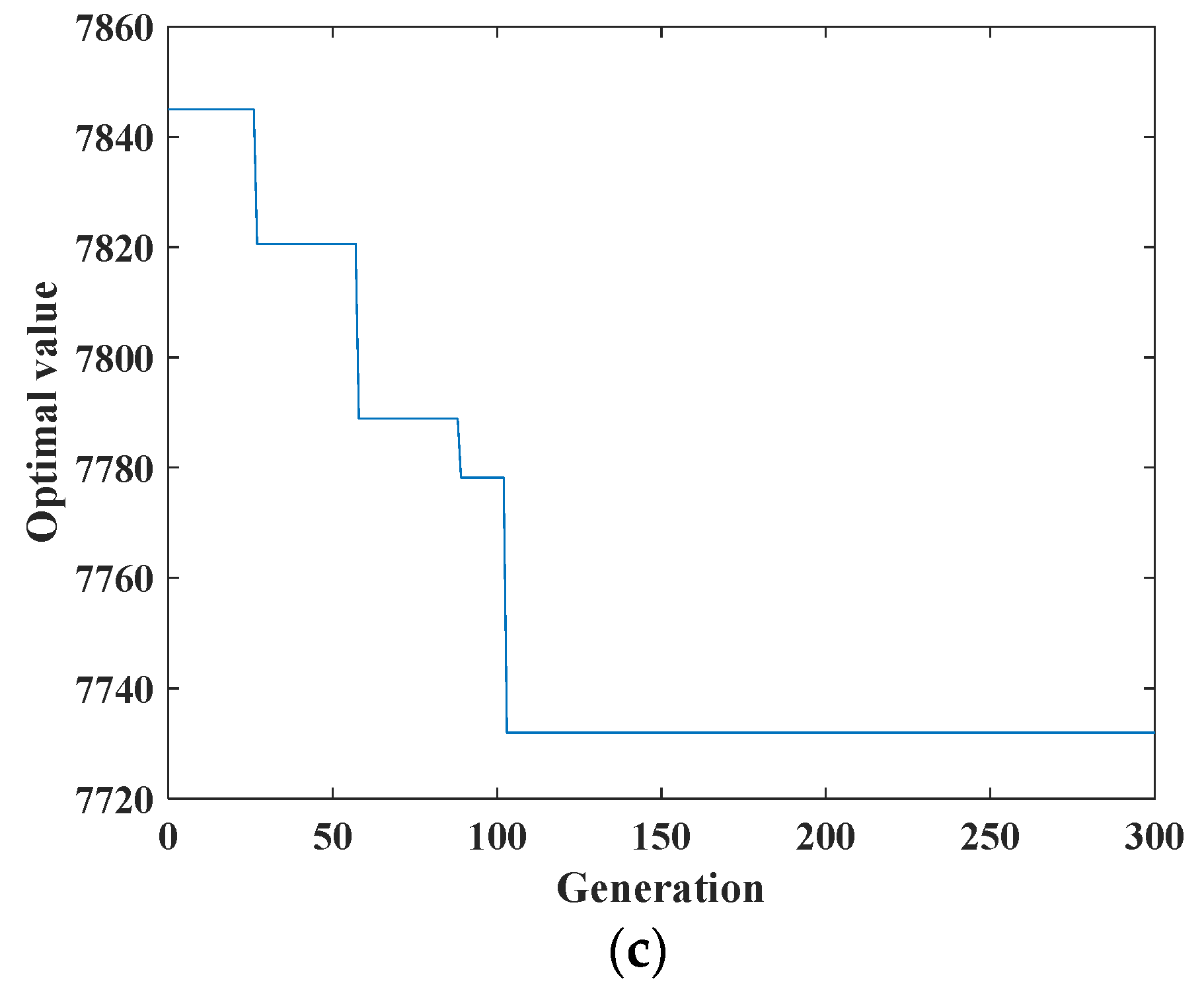
5.2.1. Speed of Convergence
5.2.2. Cost Distance
5.2.3. Feasible Solution Solving Speed
5.3. Impact of Low Carbon Constraints
- (1)
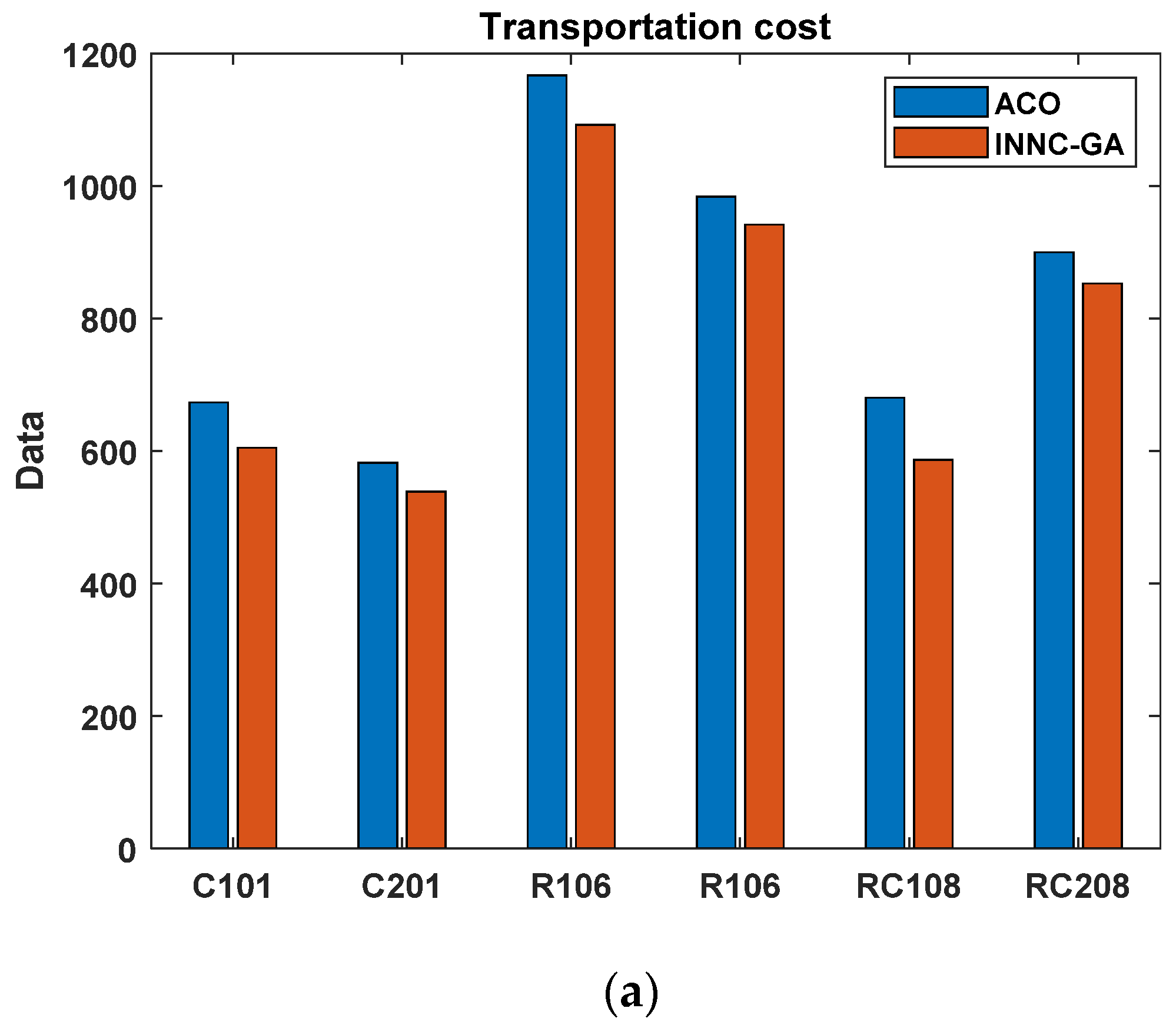
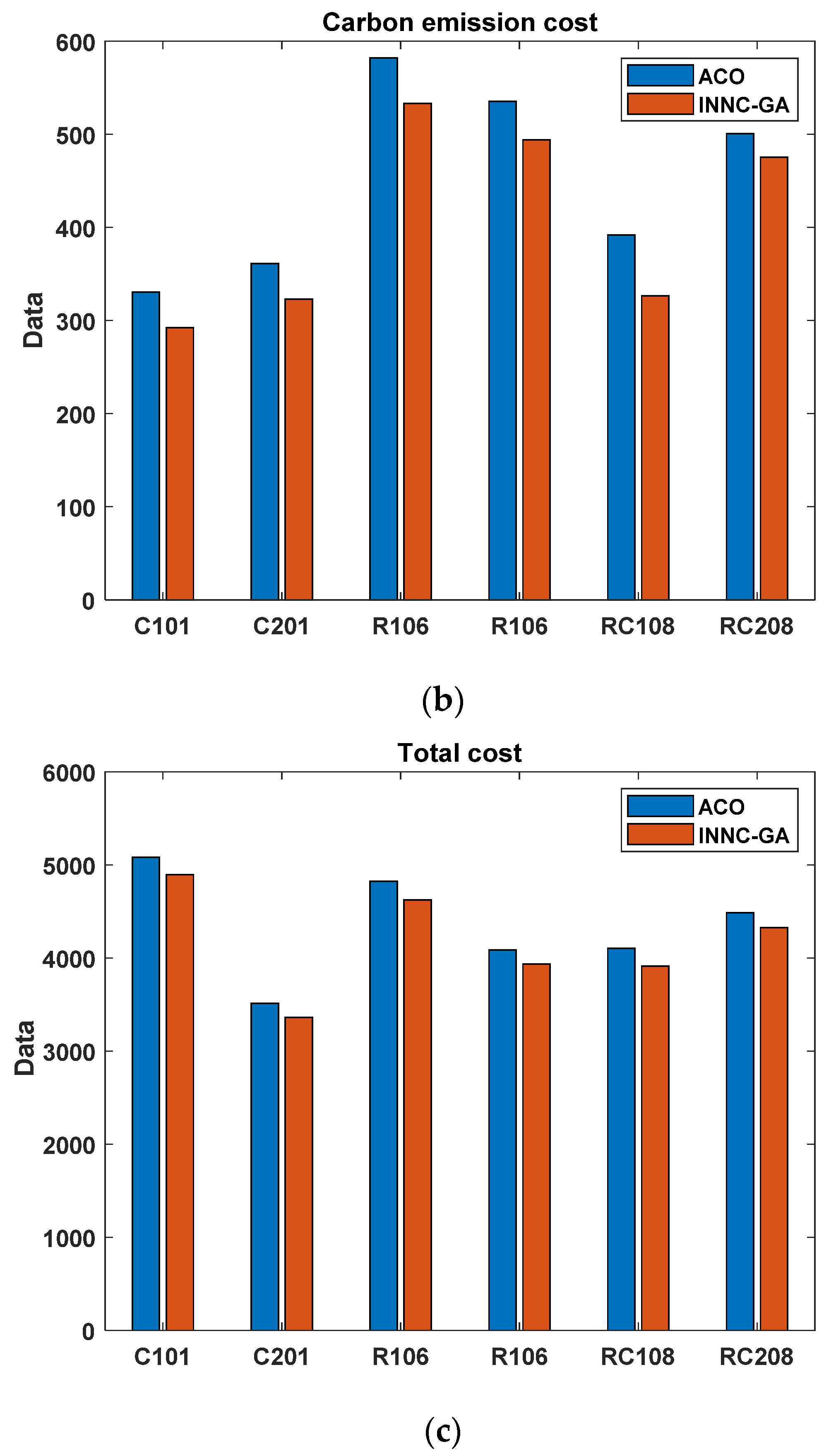
- Comparison of solution results
- (2)
- Comparison of distribution paths
5.4. Algorithm Comparison
6. Conclusions and Outlook
- (1)
- The quality of the initial solution plays a crucial role in the efficiency of the genetic algorithm. The initial solution produced by the INNC method in this study can directly generate feasible solutions that meet the constraints and exhibit a quicker convergence speed.
- (2)
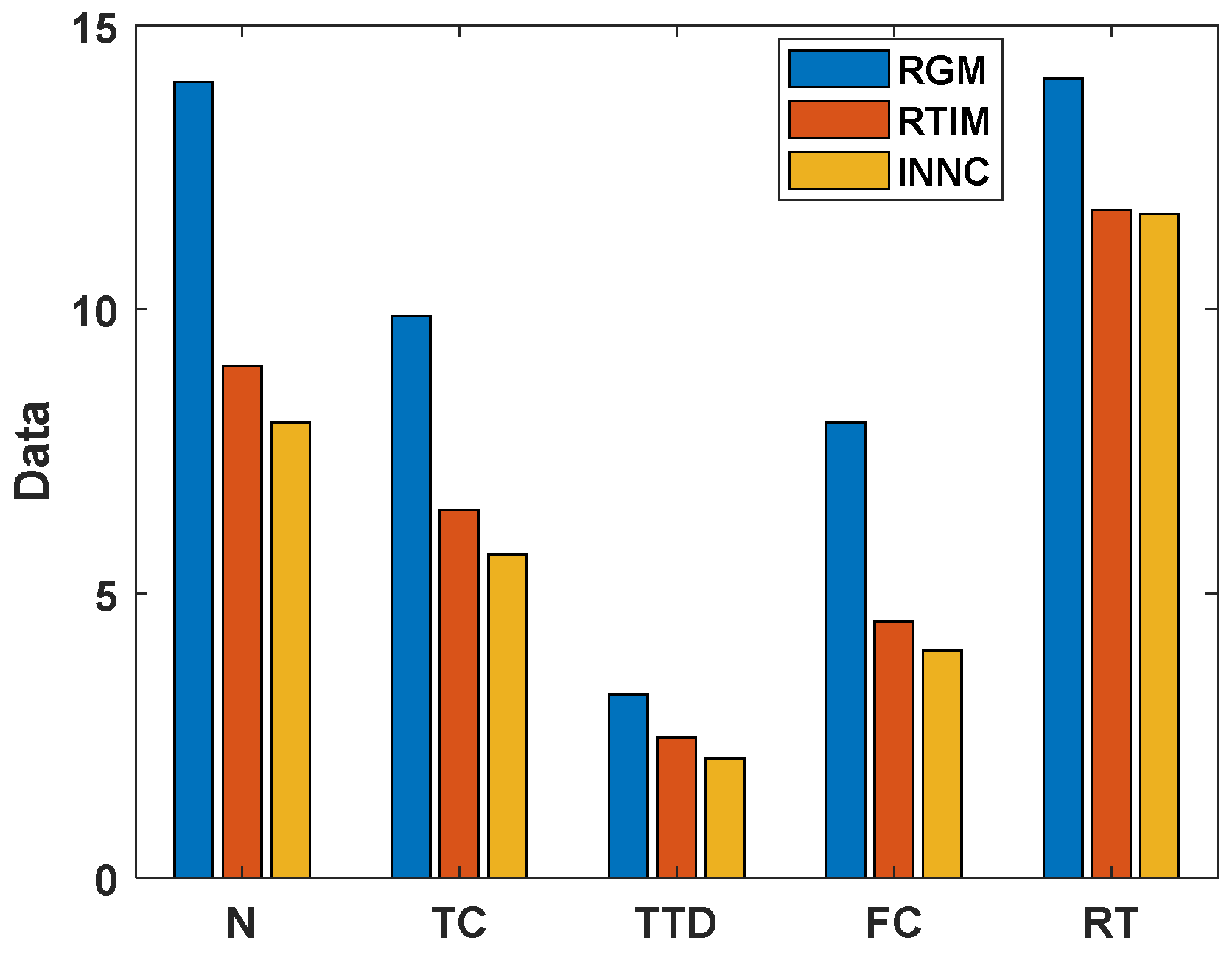
- The results of the test cases demonstrate that the genetic algorithm with INNC initial population yields superior quality initial solutions compared with the random generation and random traversal insertion methods. Furthermore, it surpasses the random generation and random traversal insertion methods in vehicle utilization, total transport distance, total cost, and running time.
- (3)
- The genetic algorithm with INNC initialization population is utilized to simulate and solve both the model without considering carbon emission costs and the model considering carbon emission costs. The results show that the model, when taking into account carbon emission costs, reduces the carbon emission cost and the total cost by an average of 4.6914% and 0.3578%, respectively, although the transportation cost increases by an average of 0.5127%. Therefore, the vehicle path model that considers carbon emissions can lower the carbon emission cost and the total distribution cost, aligning with the requirements of a low-carbon economy and offering a valuable foundation for decision-making in the logistics industry within a low-carbon economy.
Author Contributions
Funding
Institutional Review Board Statement
Informed Consent Statement
Data Availability Statement
Conflicts of Interest
References
- Ongcunaruk, W.; Ongkunaruk, P.; Janssens, G.K. Genetic algorithm for a delivery problem with mixed time windows. Comput. Ind. Eng. 2021, 159, 107478. [Google Scholar] [CrossRef]
- Wen, T.X.; Li, K.X.; Hu, Y.C. Optimization of Fresh Product Delivery Routes with Multiple Vehicle Compartments Based on Soft Time Windows. J. Highw. Transp. Res. Dev. 2023, 40, 232–238+256. [Google Scholar]
- Fallahtafti, A.; Karimi, H.; Ardjmand, E.; Ghalehkhondabi, I. Time slot management in selective pickup and delivery problem with mixed time windows. Comput. Ind. Eng. 2021, 159, 107512. [Google Scholar] [CrossRef]
- Gao, Y.; Wu, H.; Wang, W. A hybrid ant colony optimization with fireworks algorithm to solve capacitated vehicle routing problem. Appl. Intell. 2022, 53, 7326–7342. [Google Scholar] [CrossRef]
- Souza, I.P.; Boeres, M.C.S.; Moraes, R.E.N. A robust algorithm based on Differential Evolution with local search for the Capacitated Vehicle Routing Problem. Swarm Evol. Comput. 2023, 77, 101245. [Google Scholar] [CrossRef]
- Lin, N.; Shi, Y.; Zhang, T.L.; Wang, X.P. An Effective Order-Aware Hybrid Genetic Algorithm for Capacitated Vehicle Routing Problems in Internet of Things. IEEE Access 2019, 7, 86102–86114. [Google Scholar] [CrossRef]
- Prins, C. A simple and effective evolutionary algorithm for the vehicle routing problem. Comput. Oper. Res. 2004, 31, 1985–2002. [Google Scholar] [CrossRef]
- Cao, B.R.; Wang, X. Research on Optimization of Multi-Vehicle Delivery Routes Based on Dynamic Demand. Manuf. Autom. 2021, 43, 79–87. [Google Scholar]
- Chen, Y.; Dong, A.M.; Sun, Y. Road-condition-aware Dynamic Path Planning for Intelligent Vehicles. Procedia Comput. Sci. 2020, 174, 419–423. [Google Scholar] [CrossRef]
- Ge, X.L.; Ge, X.B.; Xu, J.P.; Jin, Y.Z. Research on Dynamic Vehicle Routing Problem in Multi-Channel Environment. Ind. Eng. Manag. 2022, 27, 104–117. [Google Scholar]
- Qiao, Q.; Tao, F.M.; Wu, H.L.; Yu, X.W.; Zhang, M.J. Optimization of a Capacitated Vehicle Routing Problem for Sustainable Municipal Solid Waste Collection Management Using the PSO-TS Algorithm. Int. J. Environ. Res. Public Health 2020, 17, 2163. [Google Scholar] [CrossRef] [PubMed]
- Qiu, Y.Z.; Zhang, L. Path optimization of fresh food delivery vehicles under carbon emission regulation. J. Nanjing Univ. Financ. Econ. 2021, 68–78. [Google Scholar]
- Li, J.T.; Liu, M.Y.; Liu, P.F. Optimization of cold chain logistics vehicle paths for fresh agricultural products. J. China Agric. Univ. 2021, 26, 115–123. [Google Scholar]
- Li, T.; Deng, S.J.; Lu, C.Y.; Wang, Y.; Liao, H.J. A low-carbon collection and transportation route optimization method for garbage trucks based on improved ant colony algorithm. Highw. Traffic Sci. Technol. 2023, 40, 221–227+246. [Google Scholar]
- Zhou, S.N.; Li, Z.; Wang, Z. Optimization of garbage collection and transportation routes using improved DMBSO algorithm from a low-carbon perspective. Sci. Technol. Eng. 2021, 21, 9932–9939. [Google Scholar]
- Guo, D.; Wang, J.; Zhao, J.B.; Sun, F.; Gao, S.; Li, C.D.; Li, M.H.; Li, C.C. A vehicle path planning method based on a dynamic traffic network that considers fuel consumption and emissions. Sci. Total Environ. 2019, 663, 935–943. [Google Scholar] [CrossRef] [PubMed]
- Zhang, D.Z.; Qiao, X.; Xiao, B.W.; Wang, R.D.; Mao, C.H. Multi-objective Vehicle Routing Optimization Based on Low Carbon and Stochastic Demand. J. Railw. Sci. Eng. 2021, 18, 2165–2174. [Google Scholar] [CrossRef]
- Xu, Z.S.; Wen, J.; Wang, X.; Liu, N. Research on Low-carbon Vehicle Routing Optimization of Cold Chain Logistics to Improve Refrigeration Costs-Based on ALNS Genetic Algorithm. Soft Sci. 2023, 38, 1–16. [Google Scholar] [CrossRef]
- Sun, Y.H. Research on Cold Chain Logistics Vehicle Path Problem Considering Congestion and Low Carbon. Master’s Thesis, Henan University of Technology, Zhengzhou, China, 2022. [Google Scholar]
- Zhu, Y. Research on Low-Carbon Logistics Distribution Routes Based on Improved Genetic Algorithm. Master’s Thesis, Shanxi University of Finance and Economics, Taiyuan, China, 2023. [Google Scholar]
- Zhang, J.L.; Li, C. Dynamic route optimization of distribution vehicles under the influence of carbon emission. China Manag. Sci. 2022, 30, 184–194. [Google Scholar]
- Li, Z.P.; Yang, M.Y. Research on vehicle path optimization problem based on low carbon emission. Pract. Underst. Math. 2017, 47, 44–49. [Google Scholar]


| Symbol | Definition |
|---|---|
| Node combination, , where 0 is the distribution center and 1 − n are customer points | |
| Arc set, . | |
| Vehicle set, a total of vehicles, . | |
| Distance between node and node . | |
| The nominal capacity of the vehicle. | |
| Demand of customer point . | |
| The time taken by the vehicle to travel from node to node . | |
| The moment when vehicle k arrives at customer point . | |
| The duration vehicle stays at customer point . | |
| The waiting time of vehicle k after reaching customer point . | |
| The earliest time a customer can be served. | |
| The latest service time a customer can receive. | |
| Time window of the customer. | |
| Vehicle fixed cost. | |
| Unit transport cost of vehicle . | |
| CO2 emission factor. | |
| Fuel consumption per kilometer. | |
| Carbon emissions per kilometer. | |
| Cost of carbon emissions. | |
| Fuel consumption per unit distance when empty. | |
| Fuel consumption per unit distance when fully loaded. | |
| Cost of carbon emissions per unit. | |
| Customer is serviced by vehicle . | |
| Description of symbols | |
| Vehicle travels between nodes and . | |
| 500 | (Population size) | 50 | |
| /(¥·vehicle−1) | 0.8 | (Number of iterations) | 300 |
| /(¥·km−1) | 2.63 | (Crossover probability) | 0.9 |
| /(L·km−1) | 0.16 | (mutation probability) | 0.05 |
| Model parameters. | |||
| /(¥·kg−1) | 0.76 | (generation gap) | 0.9 |
| /(kg·vehicle−1) | 200 | (penalty coefficient) | 100 |
| /(L·km−1) | 0.122 | (penalty coefficient) | 500 |
| /(L·km−1) | 0.388 | ||
| Method | Number of Vehicles(N) | Total Cost (TC) | Total Transport Distance (TTD) | Fixed Cost (FC) | Running Time (RT) |
|---|---|---|---|---|---|
| RGM | 14.00 | 9.88 K | 3.22 km | 8.00 K | 14.06 s |
| RTIM | 9.00 | 6.47 K | 2.47 km | 4.50 K | 11.74 s |
| INNC | 8.00 | 5.68 K | 2.10 km | 4.00 K | 11.68 s |
| RGM | RTIM | INNC | |
|---|---|---|---|
| The algebra of finding feasible solutions | 256 | 3 | 1 |
| Example Set | Number of Vehicles | Transportation Distance Cost | Total Cost | Carbon Emissions Cost | |
|---|---|---|---|---|---|
| X | C101 | 8 | 600.0125 | 4917.2758 | 317.2633 |
| C201 | 5 | 536.1564 | 3379.4549 | 343.2985 | |
| R106 | 6 | 1090.2500 | 4637.8854 | 547.6354 | |
| R206 | 5 | 941.6520 | 3961.8207 | 520.1687 | |
| RC108 | 6 | 576.5320 | 3930.2307 | 353.6987 | |
| RC208 | 6 | 851.2321 | 4321.4887 | 470.2566 | |
| Y | C101 | 8 | 605.0063 | 4897.1749 | 292.1686 |
| C201 | 5 | 538.6560 | 3361.7812 | 323.1253 | |
| R106 | 6 | 1092.2883 | 4625.2290 | 532.9406 | |
| R206 | 5 | 941.7303 | 3935.9300 | 494.1998 | |
| RC108 | 6 | 586.6879 | 3913.0429 | 326.3550 | |
| RC208 | 6 | 852.7563 | 4327.9224 | 475.1662 |
| Example Set | Reduction in Transportation Cost (%) | Reduction in Total Cost (%) | Reduction in Carbon Emissions Cost (%) | |
|---|---|---|---|---|
| C101 | 0.8323 | −0.4088 | −7.9097 | |
| C201 | 0.4662 | −0.5230 | −5.8763 | |
| R106 | 0.1869 | −0.2729 | −2.6833 | |
| R206 | 0.0083 | −0.6535 | −4.9924 | |
| RC108 | 1.7616 | −0.4373 | −7.7308 | |
| RC208 | −0.1791 | 0.1489 | 1.0440 | |
| Average | 0.5127 | −0.3578 | −4.6914 |
| Number of Vehicles | Customer Points | Considering the Cost of Carbon Emissions Cost |
|---|---|---|
| 1 | 10 | 0-22-24-33-31-35-37-38-9-11-10-0 |
| 2 | 13 | 0-5-2-1-7-3-4-40-44-46-45-50-43-8-0 |
| 3 | 9 | 0-6-32-49-47-42-41-48-0 |
| 4 | 11 | 0-20-30-29-34-28-26-23-18-19-15-25-0 |
| 5 | 7 | 0-27-39-36-16-14-12-17-13-21-0 |
| Number of Vehicles | Customer Points | Without Considering the Cost of Carbon Emissions Cost |
|---|---|---|
| 1 | 10 | 0-50-45-44-40-49-46-41-42-43-48-0 |
| 2 | 13 | 0-6-31-34-35-39-38-37-36-29-27-22-21-8-0 |
| 3 | 7 | 0-32-33-28-26-23-30-24-0 |
| 4 | 11 | 0-25-18-19-16-14-12-15-17-13-9-20-0 |
| 5 | 9 | 0-47-4-3-7-1-2-10-11-5-0 |
Disclaimer/Publisher’s Note: The statements, opinions and data contained in all publications are solely those of the individual author(s) and contributor(s) and not of MDPI and/or the editor(s). MDPI and/or the editor(s) disclaim responsibility for any injury to people or property resulting from any ideas, methods, instructions or products referred to in the content. |
© 2024 by the authors. Licensee MDPI, Basel, Switzerland. This article is an open access article distributed under the terms and conditions of the Creative Commons Attribution (CC BY) license (https://creativecommons.org/licenses/by/4.0/).
Share and Cite
Cheng, F.; Jia, S.; Gao, W. Low-Carbon Logistics Distribution Vehicle Routing Optimization Based on INNC-GA. Appl. Sci. 2024, 14, 3061. https://doi.org/10.3390/app14073061
Cheng F, Jia S, Gao W. Low-Carbon Logistics Distribution Vehicle Routing Optimization Based on INNC-GA. Applied Sciences. 2024; 14(7):3061. https://doi.org/10.3390/app14073061
Chicago/Turabian StyleCheng, Feng, Shuchun Jia, and Wei Gao. 2024. "Low-Carbon Logistics Distribution Vehicle Routing Optimization Based on INNC-GA" Applied Sciences 14, no. 7: 3061. https://doi.org/10.3390/app14073061
APA StyleCheng, F., Jia, S., & Gao, W. (2024). Low-Carbon Logistics Distribution Vehicle Routing Optimization Based on INNC-GA. Applied Sciences, 14(7), 3061. https://doi.org/10.3390/app14073061