1. Introduction
Sinusitis, a common medical illness defined by the inflammation of the paranasal sinuses, is a major health concern worldwide. This sinus infection affects a large number of people in various countries each year. Sinusitis occurs at a rate ranging from 16% to 21%. It is more prevalent in women and children than in men [
1]. In Saudi Arabia, it is mainly prevalent in the Eastern Province. This condition is becoming more prevalent in Saudi Arabia as a result of nasal polyposis, bronchial asthma, and analgesic intolerance [
2]. According to Hamilos [
3], chronic sinusitis reduces workplace productivity and efficiency. This has an impact on both one’s quality of life and their relationships. This is frequent in all age categories, although it is most prevalent among people aged 44 to 64.
The paranasal sinuses are divided into four pairs: maxillary, frontal, ethmoid, and sphenoid. Each sinus has unique anatomical characteristics and functions [
4]. The maxillary sinus, found in the maxilla or cheekbone, is the biggest of the paranasal sinuses. Its major role is to warm and humidify breathed air and to reduce the weight of the cranium [
5]. The maxillary sinus has a pyramidal form and drains into the nasal cavity via the ostium, which is located high on the sinus wall. In contrast, the frontal sinus is located in the frontal bone above the eyes, the ethmoid sinuses are a collection of tiny, air-filled holes between the eyes, and the sphenoid sinus lies deep within the skull behind the nose [
6]. Compared to the maxillary sinus, the frontal, ethmoid, and sphenoid sinuses have more complicated anatomical shapes and drainage channels. The frontal sinus, for example, empties into the middle meatus of the nasal cavity via the frontonasal duct [
5]. The ethmoid sinuses are labyrinthine, composed of several tiny cells that drain into the middle and superior meatuses. The sphenoid sinus empties into the sphenoethmoidal recess [
7]. The anatomical and functional distinctions between these sinuses lead to the distinct problems and pathologies identified in the maxillary sinus when compared to the other paranasal sinuses.
Untreated sinusitis can cause serious problems such as infection spreading to surrounding tissues, the development of chronic illnesses, and a negative influence on general health [
8]. Recognizing the severity of sinusitis in its early stages is critical for successful treatment and avoiding complications. The symptoms of sinusitis coincide with those of other common illnesses, such as seasonal influenza and colds, complicating the diagnosis even further. The closeness in symptoms frequently leads to a spike in referral requests for radiograph screening, putting a significant strain on healthcare resources [
8].
However, even experienced radiologists have significant challenges when interpreting these CT images. The careful examination of various sinus regions necessitates a high degree of skill and time-consuming efforts, frequently resulting in diagnostic delays and the possible loss of vital information [
9]. As the need for accurate and timely diagnoses increases, there is an urgent need to improve and streamline radiological workflow. Automating the examination of CT scans for sinus-related disorders becomes critical for addressing these problems, as it has the potential to increase diagnosis accuracy, decrease the strain on healthcare personnel, and speed up patient care.
The major goal of this study is to address the difficulties involved with diagnosing and determining the severity of sinusitis, with a particular emphasis on the maxillary sinus. Deep learning models, notably convolutional neural networks (CNNs), have demonstrated promising outcomes in medical image interpretation, including sinus-related diseases [
10]. However, the lack of balanced datasets makes it difficult to train accurate and stable models. This paper tackles this problem by using generative adversarial networks (GANs) to balance data samples [
11]. GANs serve an important function in producing synthetic pictures, which enrich the dataset and improve the performance of CNN models.
The use of GANs in medical imaging, particularly for sinus diseases, adds a new dimension to image synthesis and data augmentation [
12]. GANs help to overcome dataset size limits, improving the generalization power of deep learning models. This work investigates the use of GANs to resolve imbalances in sinusitis datasets, resulting in a more complete and diversified dataset for training.
The purpose of this study is to create customized CNN models that can not only detect sinusitis but also assess its severity using CT scans. The customized CNNs are tuned to the unique characteristics of sinus-related illnesses, allowing for a more precise and nuanced diagnosis. This study’s contribution is the unique use of GANs for data balancing and the building of CNN models specialized in severity evaluation, which advances the capabilities of deep learning in the area of sinus-related medical imaging. The contributions of this research are outlined as follows:
- i
Implement generative adversarial networks (GANs) to address data imbalance issues and enhance the dataset by generating synthetic samples, ensuring a more robust and balanced representation of various cases.
- ii
Develop and customize convolutional neural network (CNN) models specifically tailored for the diagnosis of the severity in CT images related to sinus-related pathologies, providing a targeted and optimized approach for accurate assessment and classification.
The rest of this study is structured as follows:
Section 2 introduces the relevant studies.
Section 3 elaborates on the proposed framework, dataset, and experimental design.
Section 4 demonstrates model evaluation and experimental results. In
Section 5, the conclusion and future work are discussed.
2. Related Studies
Advances in medical imaging technology and the use of advanced machine learning algorithms have led to a major increase in interest in research on sinus-related diseases and imaging modalities. In medical image analysis, convolutional neural networks (CNNs) have become the dominating force, showcasing an amazing ability in applications like sinusitis identification. Transfer learning techniques have become more popular in resolving data scarcity and improving diagnostic accuracy because they enable pre-trained models to be adapted to new datasets. Furthermore, traditional machine learning methods are still essential for classifying sinus-related pathologies. Additionally, the application of generative adversarial networks (GANs) in medical imaging has opened avenues for synthetic data augmentation, overcoming challenges associated with limited datasets and contributing to improved diagnostic performance.
2.1. Convolutional Neural Network (CNN)
CNNs, a subset of deep learning techniques, have garnered considerable attention for their remarkable efficacy in image analysis and classification tasks. Their hierarchical architecture, characterized by convolutional layers for feature extraction and pooling layers for spatial down-sampling, enables the automatic learning of intricate patterns and representations within medical images. As evidenced by various studies in the literature, CNNs have demonstrated exceptional performance in tasks ranging from detecting and diagnosing diverse medical conditions to segmenting anatomical structures with high precision. Authors have employed CNNs in the context of sinus-related pathologies and imaging modalities.
Table 1 presents a comparison of these studies.
2.2. Transfer Learning Techniques
Transfer learning is an approach to machine learning that has gained popularity because it can employ a few labeled data to apply knowledge from one task or domain to another that is similar but distinct. In the field of medical imaging, transfer learning has shown promise as a means of improving model performance and generalization in situations where data availability might be a constraint. The authors have used various applications of transfer learning in the context of diagnosing and classifying sinus-related pathologies. The comparison of transfer learning-based techniques is shown in
Table 2.
2.3. Conventional Techniques
Few authors have employed conventional machine learning techniques in the diagnosis of sinus-related conditions. Hamd et al. [
32] conducted a retrospective study focusing on predicting Maxillary Sinus Volume (MSV) using a machine learning (ML) algorithm based on data from 150 patients with normal maxillary sinuses. The study aimed to assess the predictability of the MSV using patient demographics (age, gender) and sinus length measurements in three directions. However, the study has limitations, including a small sample size and the need for enhanced training and skills to incorporate disease cases into the program for more comprehensive predictions. On the other hand, Oh et al. [
33] proposed an end-to-end process in medical imaging utilizing an independent task learning (ITL) algorithm for the diagnosis of maxillary sinusitis. The study demonstrated reasonable performance in internal and external validation tests, focusing on facial patch detection, maxillary sinusitis detection, and a fully automatic diagnosis system. Limitations included the absence of paranasal computed tomography verification for ambiguous data, such as cystic or mucosal thickening subclasses of sinusitis, and the lack of normal maxillary sinus information in training the maxillary sinusitis detector. A comparison of these studies is shown in
Table 3.
2.4. Generative Adversarial Networks in Medical Imagining
In the field of medical imaging, generative adversarial networks (GANs) have become very effective tools, providing creative ways to produce realistic and high-quality medical images. GANs make it easier to synthesize visuals in the context of medical imaging that closely imitate real patient data. This feature is especially helpful in situations where gathering a wide variety of datasets is challenging. For an array of purposes, including increasing training datasets, modeling uncommon clinical states, and improving the efficacy of diagnostic models, GANs have been used to create synthetic medical pictures. Dong Nie et al. [
34] proposed a data-driven approach using a generative adversarial network (GAN) to address the challenge of estimating computed tomography (CT) images from Magnetic Resonance Imaging (MRI) data without radiation exposure. The proposed method involves training a fully convolutional network (FCN) with an adversarial training strategy to better model the nonlinear mapping from MRI to CT. The use of an image-gradient-difference-based loss function aims to reduce blurriness in the generated CT images. Also, Guibas et al. [
35] discussed the challenges of limited and privacy-constrained medical imaging data and proposed a two-stage pipeline for generating synthetic medical images using generative adversarial networks (GANs). The focus is on overcoming data scarcity and privacy concerns by leveraging GANs to create synthetic medical images, particularly demonstrated in retinal fundi images. The pipeline involves a hierarchical generation process, separating the task into geometry and photorealism.
Most importantly, GANs also have an application in diagnosis of sinus-related conditions. For example, Kong et al. [
36] introduced a novel automation pipeline utilizing generative adversarial networks (GANs) for synthetic data augmentation, aiming to determine an optimal multiple for improving deep learning-based diagnostic performance with limited datasets. The study demonstrates superior diagnostic performance compared to conventional data augmentation using Waters’ view radiographs of patients with chronic sinusitis. However, limitations include a relatively small pool of subjects, the arbitrary choice of the auxiliary classifier GAN (ACGAN), and the omission of some conventional data augmentation methods.
Evaluating synthetic medical pictures is difficult because of the complexity and subjectivity of medical imaging. The FID score, which calculates the statistical similarity of actual and manufactured images using features extracted from a pre-trained neural network, is a quantitative measure of image quality [
11]. The SSIM measures structural similarities between images, whereas perceptual similarity considers human perception [
37]. These metrics provide a comprehensive evaluation technique that takes into account statistical, structural, and perceptual elements of picture quality.
The training procedure for GANs is an important factor impacting the quality of generated images. A GAN consists of a competitively trained generator and discriminator [
38]. During training, the generator learns to create realistic images, while the discriminator develops the ability to differentiate the difference between genuine and artificially produced images. Finding a balance between these two networks is critical for producing high-quality, realistic medical pictures.
Notably, the choice of a certain GAN architecture influences the training process as well as the quality of the produced pictures. For example, the employment of a Wasserstein GAN (WGAN) or auxiliary classifier GAN (ACGAN) requires special training techniques [
39]. The WGAN tackles mode collapse and instability difficulties by including the Wasserstein distance, resulting in more stable training [
40]. The ACGAN, on the other hand, uses auxiliary classifiers to direct the generator towards specified classes, hence improving image synthesis for specific diseases [
12].
One of the main contributions of our study is the utilization of generative adversarial networks (GANs) for synthesizing medical images, particularly for sinus-related pathologies. Also, it is clear from the above discussion that evaluating the quality of synthesized images is a challenging but critical aspect of the GAN-based image generation process. To deal with this challenge, we employed several metrics, including the Fréchet Inception Distance (FID) score, structural similarity index (SSIM), and perceptual similarity, to comprehensively assess the synthesized images.
3. Methodology
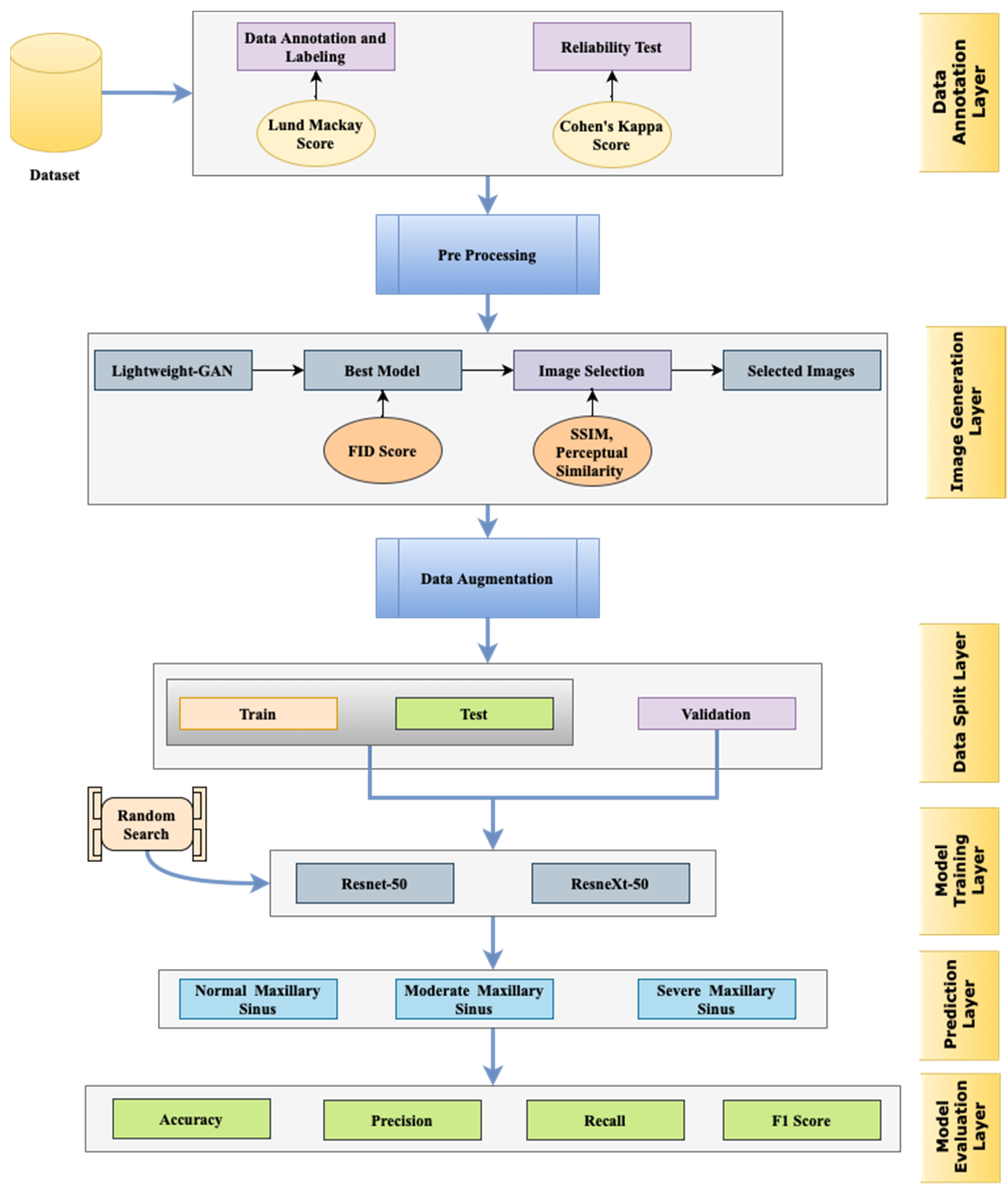
This study presents a new approach for the classification of paranasal sinus diseases, focusing mainly on maxillary sinus pathologies. Our approach leverages the capability of deep learning models, particularly generative adversarial networks (GANs) along with convolutional neural networks (CNNs), to successfully analyze medical imaging data collected from CT scans. We follow a two-stage approach whereby a lightweight GAN is used to generate synthetic data that closely resemble true sinus pathologies for data augmentation. Afterwards, the augmented dataset is applied for training and testing ResNet-50 and ResNeXt-50 models, where random search is utilized for hyperparameter tuning purposes. The utilized performance metrics are accuracy, precision, recall, and the F1-score, and the area under the ROC curve is used to determine the discriminative ability. The details of the framework are represented in
Figure 1.
The reliability of the deep learning models employed in this study is highlighted by several key factors. Firstly, rigorous pre-processing techniques were applied to the medical imaging data, ensuring high-quality input for the models. Secondly, detailed descriptions of the model architectures and hyperparameters were provided, enhancing transparency and reproducibility. Additionally, the training process was meticulously conducted, with optimization algorithms, learning rate schedules, and convergence criteria carefully selected to facilitate robust learning. Moreover, a comprehensive validation strategy, such as cross-validation, was employed to assess the models’ performance stability. The utilization of GANs further enhances reliability by facilitating data augmentation and generating synthetic data, thereby diversifying the training dataset and potentially improving model generalization. The validation of synthetic data produced by GANs involves assessing their fidelity to real data through metrics like structural similarity indices or perceptual similarity scores. This validation process ensures that the synthetic data accurately represent the characteristics of real medical images, enhancing the robustness and trustworthiness of the deep learning models employed in medical imaging tasks.
3.1. Data Collection and Generation
A total of 2142 images were collected in the form of CT scans for this study. They were obtained from two distinct healthcare institutions. The dataset utilized in this study was ethically approved by the Institutional Review Board (IRB) of the Ministry of Health, Hail, Saudi Arabia (
https://www.moh.gov.sa/en/Pages/Default.aspx, accessed on 8 December 2023)). Compliance with IRB protocols underscores the commitment to protecting patient privacy, confidentiality, and welfare, reinforcing the integrity and reliability of this study’s findings. The data were anonymized to avoid identification of the patients.
3.1.1. Imaging Modality and View
This study focused specifically on the coronal view of 2D CT images. To maintain consistency, only images with No-Contrast were included. Imaging slices with a thickness of only 0.2 mm were considered, ensuring a detailed examination of the paranasal sinuses.
3.1.2. Temporal Scope and Demographic
The data collection period spanned from 2021 to 2023, providing a contemporary representation of sinus-related pathologies. The dataset encompassed both genders, ensuring a comprehensive understanding of the diagnostic models’ performance across diverse patient groups. Patients included in the study were 18 years of age or older.
To ensure the relevance and appropriateness of the data, the following inclusion criteria were applied:
CT scans with coronal view.
2D CT images without contrast.
Slice thickness of 0.2 mm.
Patients aged 18 years and above.
3.1.3. Data Characteristics
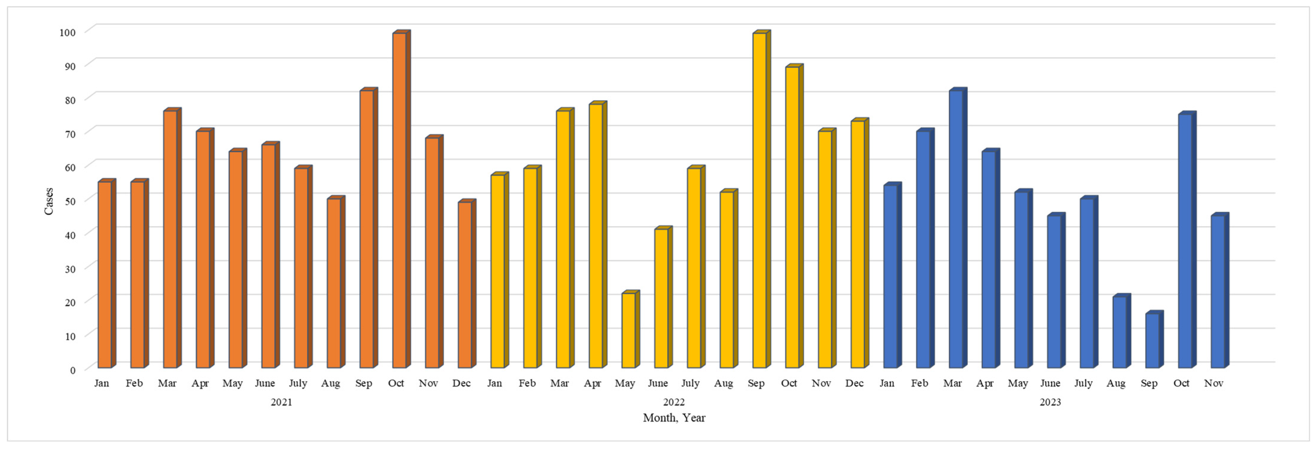
The dataset, spanning three years from 2021 to 2023, offers insights into the temporal distribution and characteristics of sinusitis cases. Encompassing 35 months, the data reveal a diverse pattern in sinusitis occurrences, indicating potential seasonality or temporal trends. The monthly counts fluctuate significantly, ranging from a minimum of 16 to a maximum of 99, suggesting susceptibility to environmental changes or viral prevalence. Each year exhibits a distinctive pattern, with 2021 starting with elevated cases, experiencing a mid-year drop, and peaking again towards the end. Notably, May 2022 stands out with a substantial decrease to 22 cases, prompting the need for further investigation into potential contributing factors. An overall increase in cases from 2021 to 2023, with the highest monthly count at 99, suggests factors like population growth or changes in reporting. Additionally, identified outliers, such as September 2023 with 16 cases, underscore the importance of understanding and addressing variations for accurate analysis and interpretation. The detail of the variation in cases is shown in
Figure 2.
3.2. Data Labeling
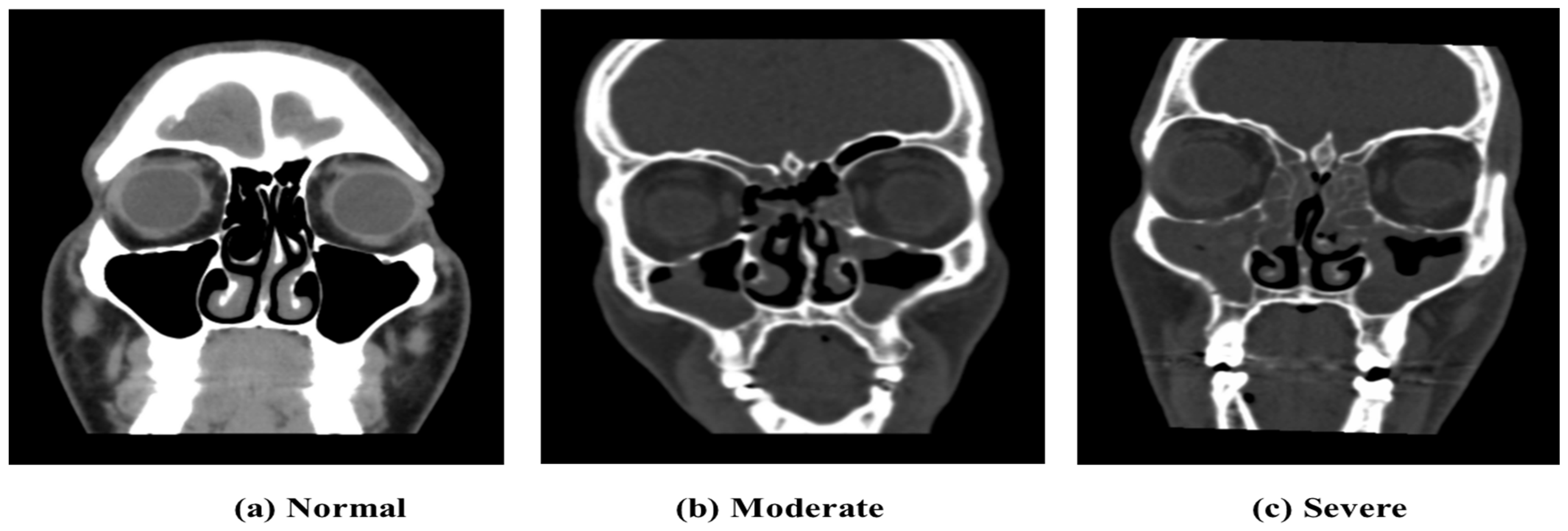
The data labeling process involved consultation with professionals in the field, including two experienced radiologists specializing in sinus-related pathologies. Out of the total 2146 collected images, 1320 images were selected to be labeled by two experienced radiologists using the Lund-Mackay rating method to quantify the severity of the images. The labeled images, taken in the coronal view, were categorized into three classes: 0 (Moderate Sinus Cases), 1 (Severe Sinus Cases), and 2 (Normal Cases), as shown in
Figure 3. After removing images of low image quality or those not belonging to the predefined categories, the final dataset comprised
n = 1320 labeled images. The Lund-Mackay scoring system is considered to be one of the most commonly used approaches to classify the severity of ethmoid sinus pathologies in the case of sinusitis [
41]. The Lund-Mackay scoring system evaluates various anatomical regions of the nasal cavity and paranasal sinuses based on the extent of opacification observed on CT scans or imaging studies. For instance, a score of 0 indicates no opacification in either maxillary sinus, while a score of 1 signifies partial opacification in one or both maxillary sinuses, and a score of 2 denotes complete opacification in one or both maxillary sinuses. Furthermore, the decision to focus on training only the Moderate and Severe classes was made to address the issue of imbalanced classes, prioritizing the severity levels that are of greater clinical relevance. The strengths of this system include the systematic and comprehensive analysis of several sinus regions, leading to an objective measure of disease severity. On the other hand, there is a limitation in its use, in its subjective interpretation, for the scoring depends on the individual differences in assessing the opacification.
For the consistency of the results, we conduct a reliability test using Cohen’s Kappa coefficient. It measures the agreement among the consultants and experts in the labeling process. Within any data labeling process such as the Lund-Mackay scoring system, Cohen’s Kappa serves as a standard metric for measuring the reliability and consistency of annotations [
42]. Its advantage lies in providing a more robust measure than a simple percentage agreement, accounting for agreements occurring by chance. However, Cohen’s Kappa can show sensitivity to differences in the category distribution, and the condition interpretation may be modified due to the rate of cases observed.
The Cohen’s Kappa (κ) statistic measures the level of agreement between two raters, with values ranging from 0 to 1. The interpretation of κ values suggests slight agreement if κ is between 0.01 and 0.20, fair agreement from 0.21 to 0.40, moderate agreement from 0.41 to 0.60, substantial agreement from 0.61 to 0.80, and almost perfect agreement from 0.81 to 1 [
42].
In the calculation of Cohen’s Kappa coefficient for inter-rater reliability, the total observations were determined by summing all values in the contingency table as shown in
Table 4, resulting in 1320. The total observed agreement, representing the sum of the diagonal values indicating agreement between the raters, amounted to 1255. Dividing the total observed agreement by the total observations yielded a proportion of 0.9515, denoted as P
o, reflecting the observed agreement rate.
To calculate the expected agreement (P
e) for Cohen’s Kappa coefficient, the proportion of agreements expected by chance for each class was computed. For Class 0, the expected agreement was determined as 189.39. Likewise, for Class 1 and Class 2, the expected agreements were calculated as 68.18 and 156.35, respectively. Summing these values provided the total expected agreement, resulting in 413.92. Dividing the total expected agreement by the total observations yielded a proportion of 0.3138 for P
e. A Cohen’s Kappa score of 0.88 was achieved among the authors using the following formula:
where
is the relative observed agreement among radiologists and
is the hypothetical probability of a chance agreement.
3.3. Pre-processing
The following 3 classes of imagery were pre-processed:
Moderate Sinus Cases (292 Images)
Normal Cases (764 Images)
Severe Sinus Cases (264 Images)
Normalization of Pixel Values: To improve the quality of the deep learning algorithms, all pixels in all images over three different classes were normalized in the range between 0.0 and 1.0. This normalization allows for improved training as well as the convergence of neural networks.
Noise Removal: In the transformation of DICOM to .png images, small artifacts, mostly of a white hue, were observed at the images’ boundaries. Using the ‘Morphology’ Python functions, these artifacts were well masked, and noise was cleaned to obtain images without artifacts.
Cropping and Padding: After noise was reduced, images were cropped to the cranial area by using the output mask from the ‘Morphology’ Python functions. Afterwards, these cropped images went through padding; 15% of the pixels were filled with a black color. This pre-processing step which is considered being important before inputting the images into the deep learning algorithms aids in the maintenance of the consistency of the input dimensions. The obtained images reveal the cropped-pad image format that is optimal as input for the algorithm. Nevertheless, it is understood that automatically extracting the sinus area in all images presents challenges due to variations in the size of human cranial areas and potential omissions in specific portions of the sinus.
3.4. Image Generation Using GANs
We employed generative adversarial networks (GANs) to generate synthetic images, focusing on two distinct classes: Moderate and Severe sinusitis. The Moderate class comprised 292 images, each undergoing a standardized image pre-processing pipeline. Post-processing, every image was resized to dimensions of 128 × 128 × 3 (width × height × number of channels). This uniform resizing ensured consistent input dimensions for subsequent stages in the image generation process. Similarly, the Severe class encompassed 264 images, and similar to the Moderate class, each image underwent resizing to 128 × 128 × 3 dimensions during pre-processing. This standardized sizing facilitated the integration of both classes into the image generation pipeline.
3.4.1. Lightweight GAN
Although generative adversarial networks (GANs) are very promising in artificial image synthesis, the training process has various challenges associated with stability and speed. As part of optimizing the image generation, various GAN architectures like the DCGAN and WGAN [
40,
43] were employed. However, maintaining consistently stable conditions during training was still a major challenge.
In order to overcome the problems of training stability, a lightweight GAN variant was considered. The lightweight GAN integrates the Skip-Layer channel-wise Excitation (SLE) module, utilizing low-scale activations to enhance channel responses on high-scale feature-maps. This design facilitates robust gradient flow, expediting model training and enabling automated style and content disentanglement similar to StyleGAN2. Additionally, a self-supervised discriminator (D), serving as a feature-encoder with an extra decoder, is introduced for more descriptive feature-map learning, particularly through auto-encoding strategies. The self-supervised discriminator (D) used in this study includes two decoders designed for feature-maps on two scales: f1 at 162 and f2 at 82. Each decoder comprises four convolutional layers, generating images at a resolution of 128 × 128, resulting in minimal additional computational burden compared to other regularization methods. We employ random cropping on f1, extracting 1/8 of its height and width, and similarly crop the real image to obtain the I part. After resizing the real image to match, the decoders produce the I0 part from the cropped f1 and I’ from f2. Finally, D and the decoders are jointly trained to minimize the loss by aligning the I’ part with the I part and I’ with I.
This efficient GAN model had many benefits, such as faster training time, less hardware requirements, and better performance in producing artificial images [
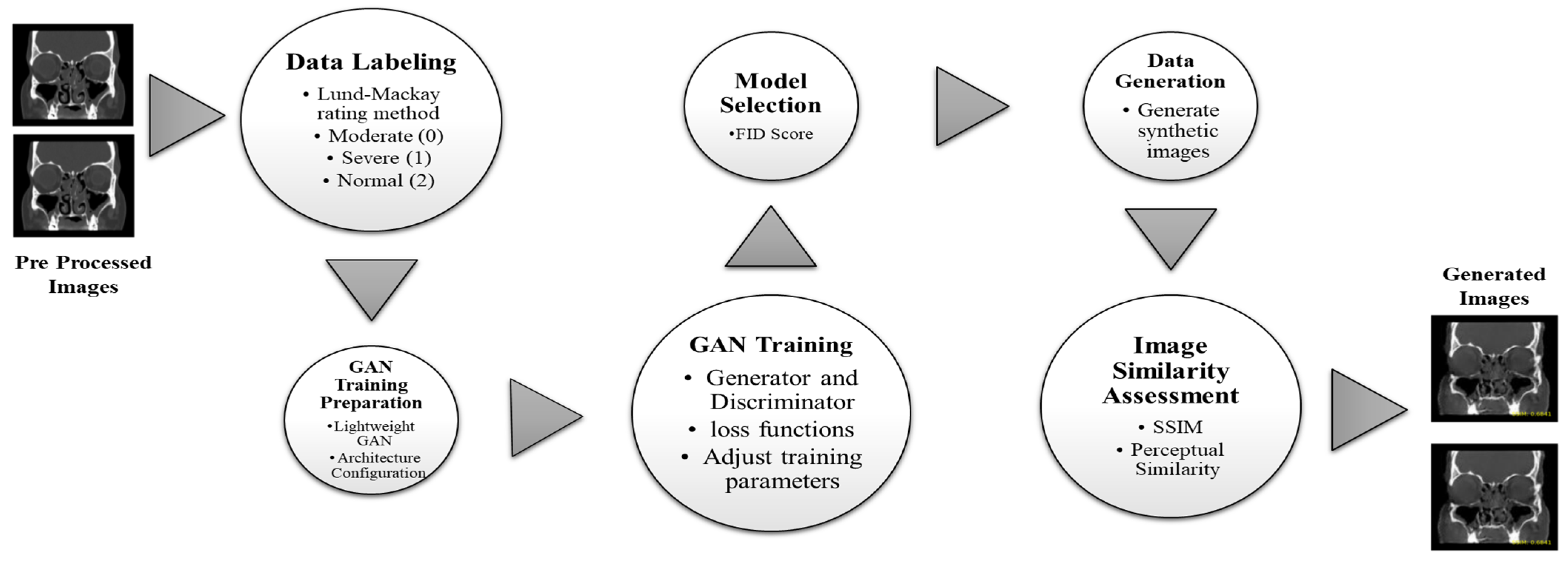
44]. The lightweight GAN that was created for seamless operations turned out to be effective in the context of sinusitis severity classification. One key advantage of adopting such a typical GAN is based on reducing the data samples during training to produce images substantially far compared with different types. Although some GAN variants need larger datasets for convergence, the lightweight version implemented in this study is still able to learn efficiently from limited data [
44]. While the lightweight GAN presents advantages in terms of speed and efficiency, its limitations include a potential trade-off in the richness of image generation compared to more intricate GAN architectures. The still-challenging aspect to balance is that of the trade-off between computational efficiency and image quality. The image generation flow using the GAN is shown in
Figure 4.
Training of Lightweight GAN
In the training of the lightweight GAN, both the generator and the discriminator operate concurrently. The generator produces synthetic (fake) data, while the discriminator distinguishes between real and fake data. The training aims to strike a balance where the generator can effectively fool the discriminator, and the discriminator accurately classifies the data. An imbalance may occur if the discriminator becomes too strong relative to the generator, hindering the generation of realistic synthetic data. To address this, adjustments such as modifying learning rates and adding augmentations are implemented during training. The ultimate goal is to reach a state where the generator produces highly realistic data, challenging the discriminator’s ability to differentiate between real and fake data. In the training process for the ‘Moderate’ class, adjustments were made at step 50,000, including further reducing the learning rate and increasing the augmentation to 0.9. Two additional augmentation types, color and offset, were introduced to enhance the similarity between output and true input images. Training continued with these parameters until Epoch 100, lasting approximately 32 h. The training parameters for the ‘Moderate’ and ‘Severe’ classes are summarized in
Table 5.
Evaluation Metrics
The following evaluation metrics were used in the training of the lightweight GAN:
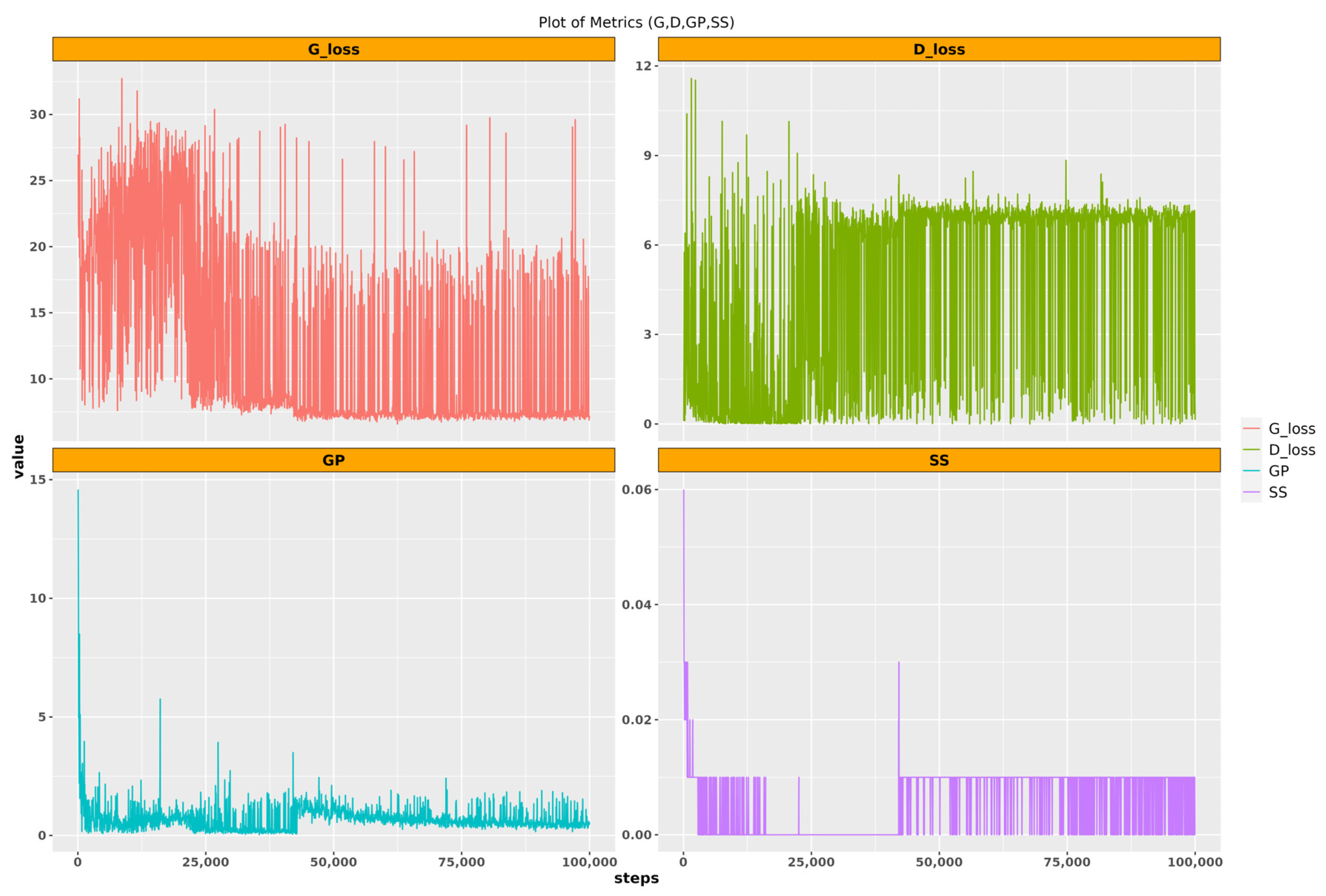
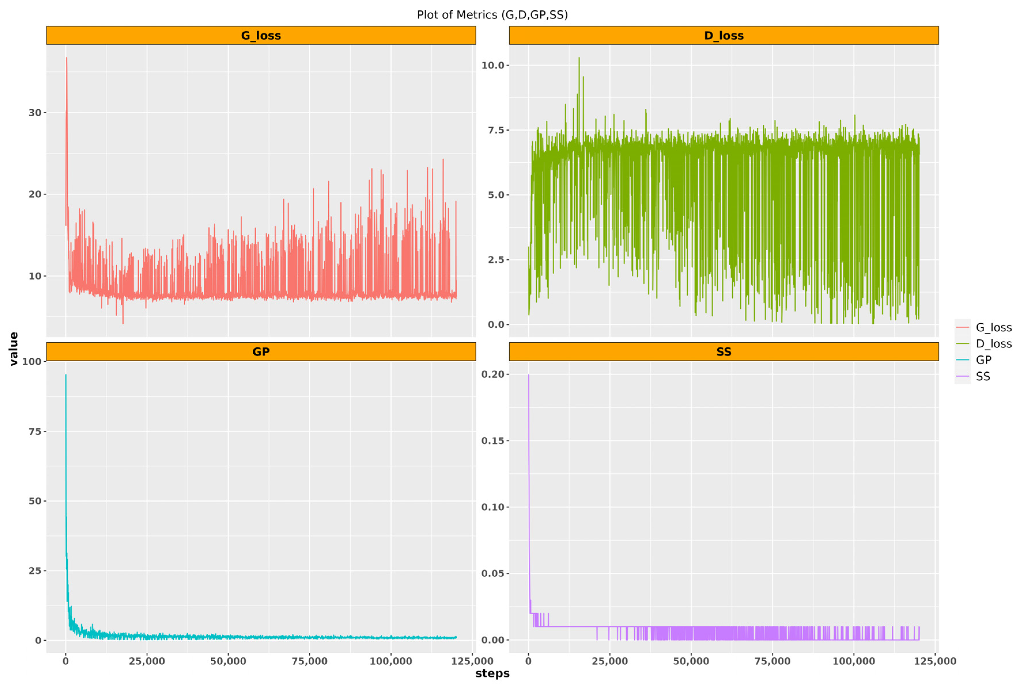
‘D’ represents the discriminator loss, indicating how effectively the discriminator distinguishes between real and generated data; lower values signify superior performance. Conversely, ‘G’ denotes the generator loss, reflecting the generator’s ability to produce data indistinguishable from real data; lower generator loss values indicate better performance. ‘GP’ signifies Gradient Penalty, a regularization technique crucial for stabilizing discriminator training in Wasserstein GANs by ensuring gradients are close to 1, thereby mitigating mode collapse and enhancing training stability. Finally, ‘SS’ represents the self-supervised learning loss, utilized in lightweight GANs to facilitate the discriminator’s learning of data representations; lower SS loss values indicate improved performance in this self-supervised learning process.
A low discriminator loss might indicate that the discriminator is performing well, but if the generator loss is very high, this could suggest that the generator is not able to fool the discriminator, which might result in poor-quality generated images. Similarly, a low self-supervised loss might suggest that the discriminator is learning useful representations of the data, but this does not necessarily guarantee that these representations will result in high-quality generated images.
Recognizing the impact of the variability induced by the small size of the input images in the training process, two data generation phases were incorporated. Firstly, during the 100,000 training steps for the ‘Moderate’ class, 100 models were systematically saved to a designated directory. For each of these saved models, a total of 292 images were generated, aligning with the number of true images. Similarly, for the ‘Severe’ class, a data generation phase was implemented during the 120,000 training steps, saving 120 models. Correspondingly, for each saved model, 264 images were generated, mirroring the number of true images. These iterative data generation processes aimed to address the variability in the generator and discriminator loss and capture the intricacies of the training dynamics, ultimately producing synthetic images that comprehensively represent the diversity inherent in the training dataset. The visualization of the performance evaluation metrics in both classes is shown in
Figure 5 and
Figure 6.
3.4.2. Best Model Selection
For both the ‘Moderate’ and ‘Severe’ classes, the selection of the 10 best-performing models was based on the Fréchet Inception Distance (FID). It is a quantitative measure employed to assess the quality and diversity of images that are ultimately generated by generative adversarial networks. It measures the similarity between two sets of images, namely the set of real images and the set of generated images. The value of the FID score depends on the particular feature representations obtained from a pre-trained deep convolutional neural network, for example Inception v3.
The Fréchet Inception Distance (FID) equation is represented as follows:
where
represents the squared Fréchet distance,
denotes the squared Euclidean distance between the means u
1 and u
2 of the feature distributions, and
calculates the trace of the covariance matrices
, along with their element-wise multiplication and square root operations.
It is important to note that the FID score ranges from 0 to infinity, with 0 indicating identical sets of images. A lower FID score suggests better image quality and greater similarity to the original image set. However, the FID score does not evaluate the semantic meaning or domain-specific characteristics of the images; it solely measures the statistical similarity between two sets of images. The selection process involved identifying the 10 models with the lowest FID scores from the 100 and 120 saved models for the ‘Moderate’ and ‘Severe’ classes, respectively. This rigorous evaluation method aimed to ensure the quality and similarity of the generated images to the real dataset. The FID score of the Moderate and Severe classes for the 100 and 120 saved models is shown in
Figure 7.
3.4.3. Selection of Generated Images
To ensure the selection of generated images closely resembling the true images in terms of similarity, two key metrics were employed with the 10 best-selected models:
- i
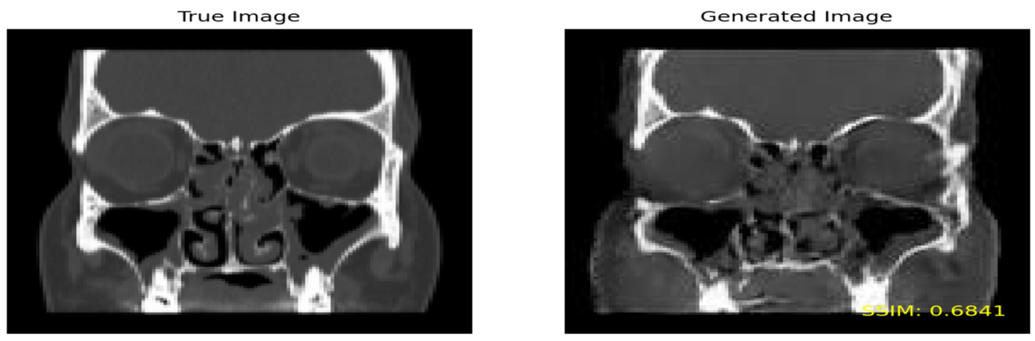
Structural Similarity Index (SSIM): The SSIM is a metric used to quantify the similarity between two images by comparing their luminance, contrast, and structure. The SSIM scores range from 0 to 1, with higher scores denoting greater similarity. This metric is widely utilized for evaluating the quality of generated images, particularly those produced by generative adversarial networks (GANs). Beyond applications in GANs, the SSIM finds use in diverse domains such as image compression and enhancement.
- ii
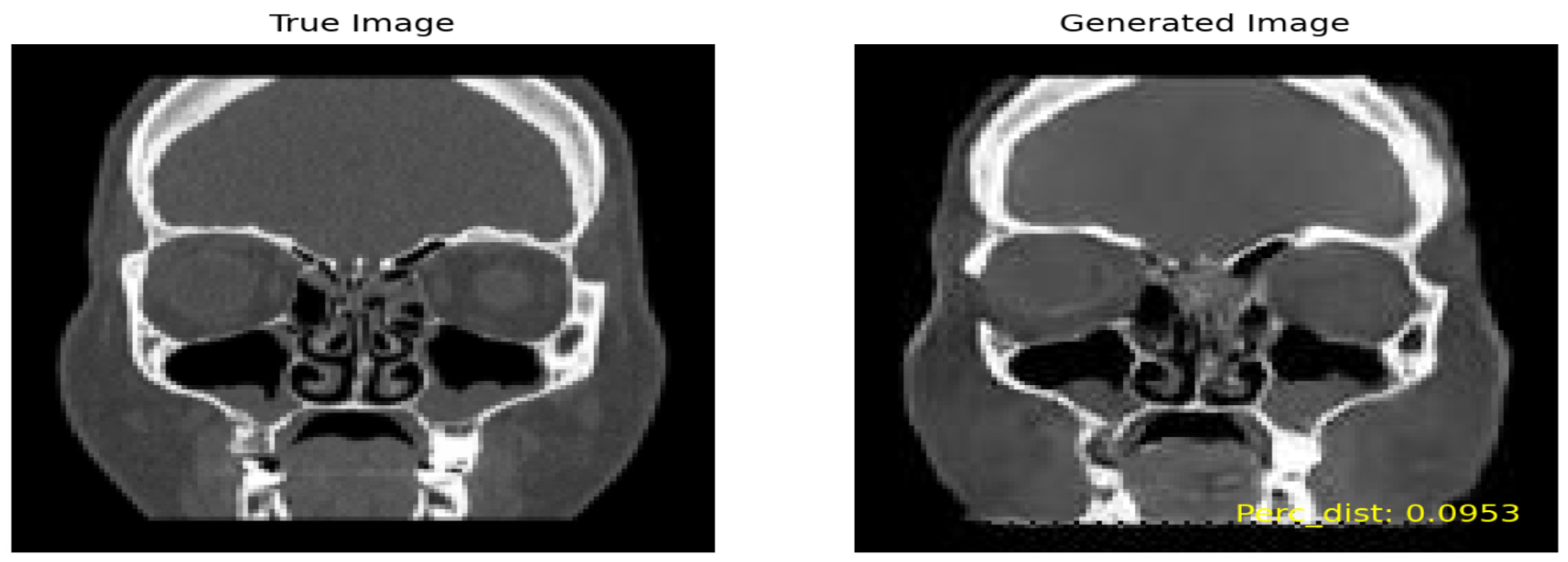
Perceptual Similarity: In contrast to the SSIM, which measures the overall similarity between two images, perceptual similarity assesses how similar images are perceived by humans. This means that a fake image exhibiting high visual resemblance to a true image may receive a high perceptual similarity score, even if its structural similarity score is comparatively low.
Figure 8 shows the true image on the left and the generated image on the right by including the
SSIM value on the lower part of the image.
In the evaluation process for the ‘Moderate’ class, an SSIM threshold of 0.6 and above was applied to retain the generated images displaying the highest similarity to the true images. Out of a total of 852,640 combinations, 717 images exhibited a similarity greater than 0.6 and were consequently selected.
Similarly, for the ‘Severe’ class, an SSIM threshold of 0.475 and higher was employed to preserve the generated images with the utmost similarity to the true images. Among the 693,079 combinations considered, 703 images surpassed the 0.6 similarity threshold and were chosen for further analysis.
Figure 9 shows the true image on the left and the generated image on the right by including high perceptual similarity.
Following a similar methodology as employed for the SSIM, we conducted a thorough similarity assessment using the perceptual metric. For the ‘Moderate’ class, with an initial pool of 852,640 combinations, 1523 images were generated, adhering to a threshold of 0.175. In the case of the ‘Severe’ class, involving 693,079 combinations, a set of 1665 images was generated, applying a threshold of 0.2035.
3.4.4. Selected Metric
The choice of different thresholds for the ‘Moderate’ and ‘Severe’ classes stemmed from the observed disparity in the quality of generated images by the lightweight GAN. The FID plot further validated this, showcasing consistently lower FID scores for the ‘Moderate’ class, indicating superior image quality compared to the ‘Severe’ class across all saved models. Leveraging the perceptual similarity metric allowed us to meticulously select generated images that closely mirrored the quality of true images. This metric was deemed crucial for the subsequent classification task due to its effectiveness in capturing nuanced visual similarities. After the selection of 1523 and 1665 images for the ‘Moderate’ and ‘Severe’ classes, respectively, a critical step involved the removal of duplicate images. This precautionary measure was essential as multiple generated images exhibited high similarity to a single true image. Following the removal of duplicates, the dataset was refined to comprise 794 generated images for the ‘Moderate’ class and 411 generated images for the ‘Severe’ class, ensuring a diverse and non-redundant dataset for the subsequent classification model training.
Table 6 present the proportions of each class respectively.
3.4.5. Data Split
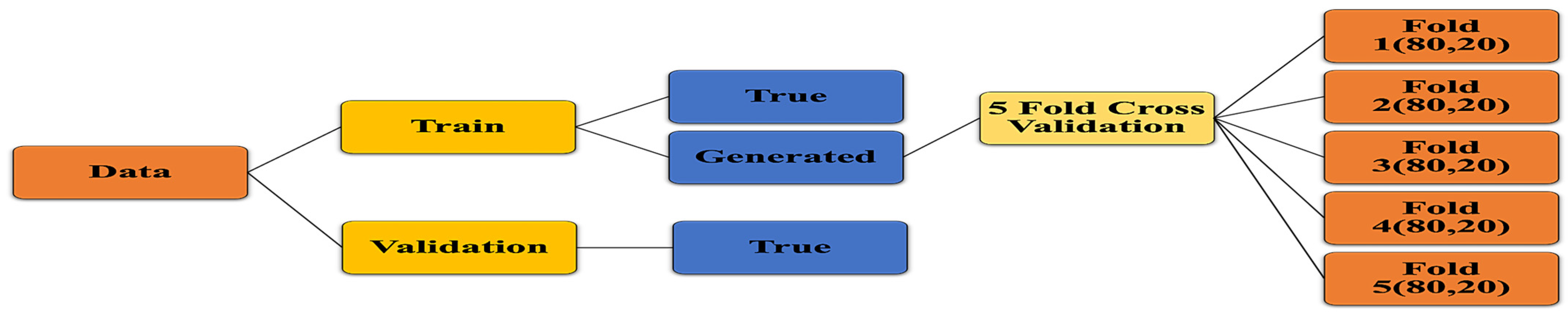
The data split for training the deep learning algorithms involved partitioning the dataset into two main subsets: train and validation as shown in
Figure 10. The train set comprised both true and generated images, with 1216 true images and 1205 generated images. Additionally, a validation set consisting of 104 true images was set aside to assess the performance of the trained models. To ensure the robustness and generalization of the models, a 5-fold cross-validation strategy was adopted for the train data, with each fold containing 80% train and 20% test data. For the validation dataset, a small proportion of approximately 8% of the true images was allocated. This decision was made due to the limited size of the dataset, aiming to maximize the number of images available for training. Specifically, the validation data comprised true images selected from all three classes (Moderate, Severe, Normal), focusing on those that exhibited the least similarity with the generated images.
The generation of the validation set involved a meticulous process to ensure its representativeness and effectiveness in evaluating model performance. As discussed previously, the lightweight GAN was trained using all images from the Moderate and Severe classes to produce generated images. These generated images were then filtered to retain only those most similar to the true images, based on a threshold of 0.175 for the Moderate class, resulting in 1523 generated images. Subsequently, unique generated images were selected, yielding a set of 152 images closely resembling the true images of the Moderate class. Similarly, for the Severe class, 169 true images were identified to be highly similar to the generated ones out of the initial 264. To form the validation dataset, a pragmatic approach was adopted, excluding the 152 images from the Moderate class and 169 images from the Severe class. Then, a random selection of 10% of the remaining true images from each class was chosen as validation data. This method ensured that the validation set contained representative samples from each class while mitigating the computational complexity associated with computing perceptual metrics. The details of the validation set are listed in
Table 7.
3.4.6. Transfer Learning Models
In this study, we utilize the transfer learning approach for classification. ResNet-50 and ResNeXt-50 are used for the classification of sinusitis severity from CT images. Leveraging the learned features from large-scale datasets, these models offer a powerful framework for extracting relevant features and achieving robust performance in medical image analysis tasks.
Additionally, we incorporated several augmentations during the training process to further diversify our dataset. These augmentations, listed in
Table 8, include rotation with a range of 20 degrees, horizontal and vertical shifts with a range of 0.15, horizontal flipping, nearest neighbor filling mode, zooming with a range of 0.1, and shearing with a range of 0.15.
ResNet-50
ResNet-50, or Residual Network with 50 layers, is a deep convolutional neural network architecture developed by He et al. [
45]. It is a member of the ResNet family, which is recognized for its novel method of leveraging residual connections to solve the vanishing gradient problem during training. ResNet-50’s core architecture includes 50 layers, which include convolutional, pooling, and fully connected layers [
45]. ResNet’s distinguishing characteristic is the use of skip connections or shortcuts to bypass one or more levels, allowing the network to learn residual mappings. These residual connections make it easier to train very deep networks by allowing for the direct passage of gradients during backpropagation, addressing the degradation problem that standard deep networks encounter.
ResNet-50 was chosen because of its shown performance in a variety of computer vision applications, such as imagine classification, object identification, and image segmentation [
46,
47]. Its deep design allows it to learn nuanced characteristics from images, making it appropriate for challenging tasks like sinusitis severity categorization using CT scans.
ResNeXt-50
ResNeXt-50 is a modified version of the ResNet architecture, which was developed by Xie et al. [
48]. It draws on the ResNet design philosophy, but adds an additional concept called cardinality to increase the model’s representational capability [
48]. ResNeXt-50 has a similar design to ResNet-50, consisting of several residual blocks linked together via skip connections. However, ResNeXt-50 adds a new dimension to the architecture: cardinality, which reflects the number of distinct pathways within each residual block. ResNeXt-50 improves model performance by increasing cardinality, which increases the model’s ability to collect varied characteristics and patterns from input data. ResNeXt-50 outperforms typical ResNet designs in terms of generalization and scalability because of the additional parallelism afforded by many pathways inside each block [
48].
Just like ResNet-50, ResNeXt-50 is also chosen for its high performance and scalability in a variety of computer vision workloads. Its capacity to capture a variety of characteristics makes it ideal for tasks that need complicated and heterogeneous data, such as medical image analysis [
49,
50]. ResNeXt-50, like ResNet, has pre-trained versions that allow for quick transfer learning and adaption to specific tasks with little labeled input.
3.4.7. Hyperparameters
In this study, the hyperparameters for the model tuning of both ResNet-50 and ResNeXt-50 are initialized to optimize the classification models. These hyperparameters, including the number of dense layers, hidden units within these layers, dropout rate, and choice of optimizer, collectively influence the neural network’s architecture and training optimization, as shown in
Table 9. The number of dense layers, ranging from 1 to 2, determines the depth and complexity of the network, while the hidden units define the dimensionality of the layer’s output space, aiding in capturing intricate patterns. Dropout regularization, applied with rates between 0.2 and 0.3, mitigates overfitting by randomly deactivating neurons during training. The choice of optimizer, “Adam” or “AdamW”, further influences the model’s convergence speed and robustness during the training process. These hyperparameters play pivotal roles in enhancing the model’s capacity and generalization performance, crucial for achieving optimal results in the classification task.
Optimal Hyperparameters
In this study, the process of determining optimal hyperparameters for both ResNet-50 and ResNeXt-50 models involved the utilization of random search instead of Bayesian Optimization and Hyperband. Random search was chosen due to its simplicity, ease of implementation, and effectiveness in exploring the hyperparameter space, particularly when the search space is not excessively large.
The optimal hyperparameters for both ResNet-50 and ResNeXt-50 models were identified to enhance their performance in terms of classification accuracy and convergence speed, as shown in
Table 10. For ResNet-50, the optimal configuration included a single dense layer with 288 hidden units, coupled with a dropout rate of 0.3, and employing the “Adam” optimizer. Similarly, the optimal setup for ResNeXt-50 comprised a single dense layer with 384 hidden units, a dropout rate of 0.3, and the utilization of the “Adam” optimizer. For the optimal parameters, the Accuracy Score achieved was 95.3% for ResNet-50 and 96.23% for ResNeXt-50.
3.5. Experimental Setup
The experimental setup for this research was conducted utilizing Google Colab Pro+ with GPU T4 acceleration. Leveraging the computational power offered by Google Colab Pro+ and GPU T4, we implemented the training and evaluation of the proposed deep learning models, ResNet-50 and ResNeXt-50, for the classification of sinus pathologies. The Keras-Tuner Python package was employed for hyperparameter tuning, enabling an automated and efficient search for optimal model configurations.
4. Results
This section encapsulates the culmination of our study’s findings, providing a comprehensive analysis and interpretation of the experimental outcomes. In this section, we delve into the performance metrics, model evaluations, and statistical analyses obtained from our deep learning models, ResNet-50 and ResNeXt-50, trained for the classification of sinus pathologies.
4.1. Confusion Metrics
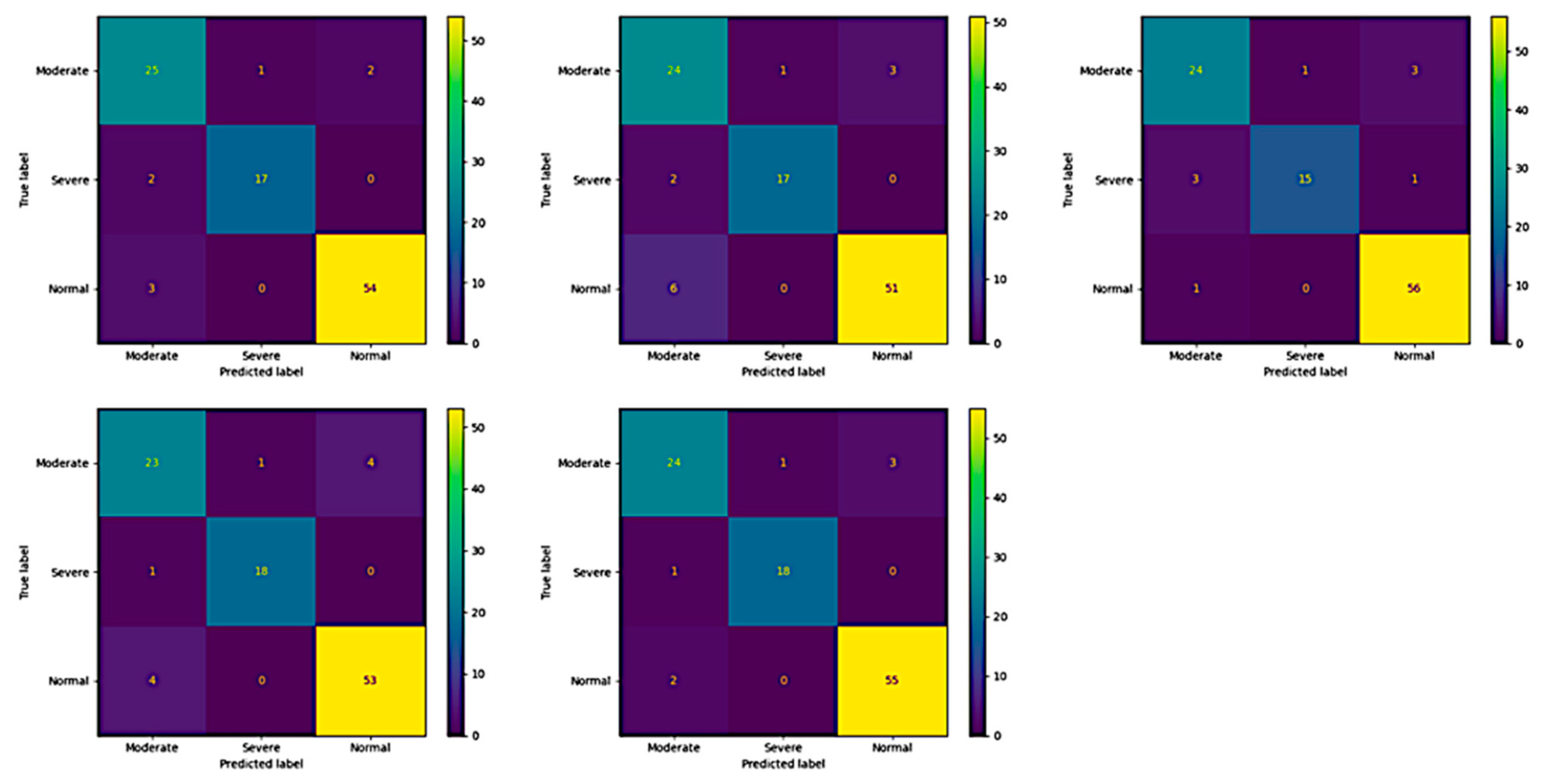
The confusion matrix shows the performance of the ResNet-50 and ResNeXt-50 models on a validation dataset, to show the model’s generalizability and ability to correctly classify instances and identify any misclassifications or errors in the predictions.
Across all five folds of the validation process, the ResNet-50 model consistently demonstrated strong predictive performance in classifying maxillary sinus. Notably, the model achieved high accuracy in identifying “Moderate” and “Severe” cases, with the best results observed in Folds 1, 2, 4, and 5, where it accurately predicted 25 out of 28 true “Moderate” cases and all 17 true “Severe” cases. Moreover, the model exhibited remarkable consistency in distinguishing between different severity levels, maintaining minimal misclassifications in both “Moderate” and “Severe” categories across all folds. Although, the model encountered slight challenges in accurately identifying “Normal” cases, particularly in Folds 1 and 2, where it misclassified only 3 and 6 instances out of 57, respectively. The details of the validation confusion matrix of ResNet-50 is shown in
Figure 11.
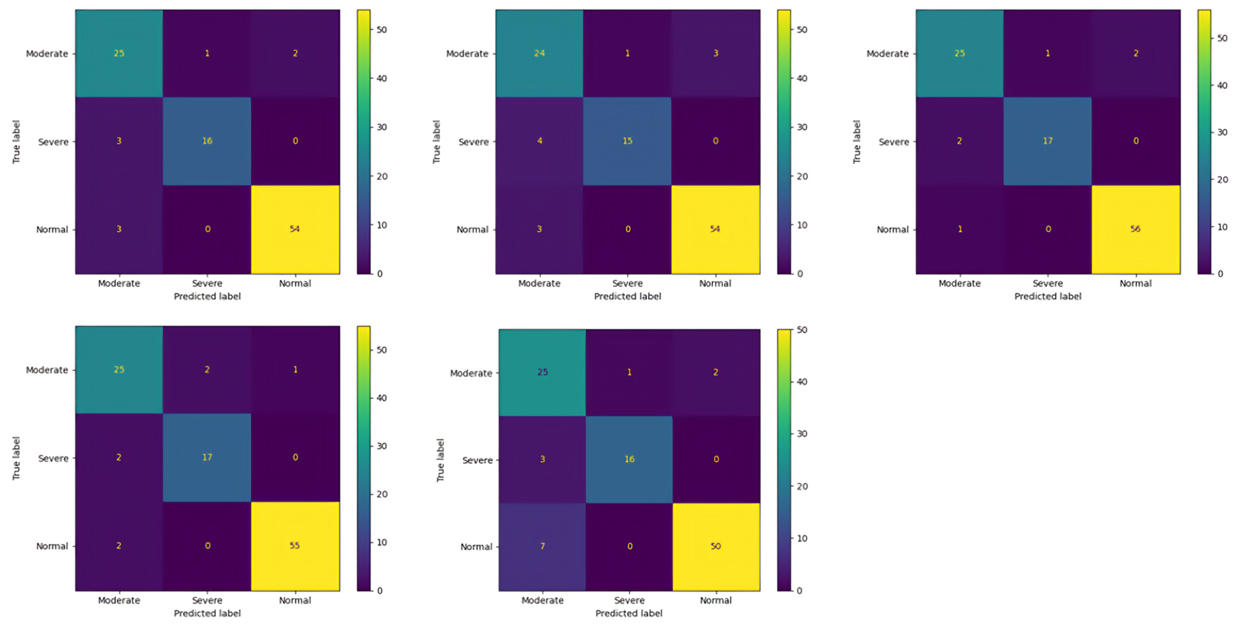
Similarly, in the validation confusion matrices of Fold 1 to Fold 5 for ResNeXt-50, the model consistently demonstrates strong performance in accurately identifying “Moderate” and “Severe” cases, with few misclassifications observed. Across all folds, the model correctly predicts the majority of “Moderate” cases, ranging from 24 to 25 out of 28 true instances. Similarly, for “Severe” cases, the model maintains high accuracy, correctly classifying between 15 and 17 out of 19 true cases in each fold. However, the model encounters challenges in accurately distinguishing “Normal” cases, with misclassifications ranging from 0 to 3 instances across the folds. Notably, the model’s misclassifications primarily involve “Normal” cases being incorrectly labeled as “Moderate”, indicating a potential overlap in features between these categories. The details of the validation confusion matrix of ResNeXt-50 are shown in
Figure 12.
4.2. Train
For the training dataset, both ResNet and ResNeXt-50 models demonstrated excellent performance across all evaluation metrics. ResNeXt-50 achieved a slightly lower loss of 0.088 compared to ResNet’s 0.111, indicating better optimization during training. Similarly, ResNeXt-50 outperformed ResNet in accuracy, precision, recall, and the F1-score, achieving values of 97.047%, 0.971, 0.970, and 0.970, respectively, compared to ResNet’s 96.448%, 0.965, 0.964, and 0.964. The superior performance of ResNeXt-50 in the training set suggests its ability to capture more intricate patterns and generalize well to the training data.
4.3. Test
In the testing phase, both models maintained high accuracy, precision, recall, and F1-score. ResNeXt-50 continued to exhibit a slightly lower loss (0.180) compared to ResNet (0.174), suggesting better generalization to unseen data. However, ResNet demonstrated marginally higher accuracy (0.952) and precision (0.954) compared to ResNeXt-50 (0.949 and 0.951, respectively). The recall and F1-score were similar between the two models, indicating their robustness in correctly identifying positive instances and achieving a balance between precision and recall.
4.4. Validation
In the validation dataset, both ResNet and ResNeXt-50 models exhibited comparable performance. As shown in
Table 11, ResNet achieved a loss of 0.297, while ResNeXt-50 achieved a slightly lower loss of 0.285. However, ResNeXt-50 demonstrated marginally higher accuracy (0.911) and precision (0.917) compared to ResNet (0.915 and 0.913, respectively). The recall and F1-score were consistent across both models, indicating their ability to generalize well to new, unseen data. Despite minor variations, both models showcased robust performance in the validation set, reaffirming their effectiveness in real-world applications.
It is clear from above that ResNeXt-50 demonstrated superior performance across all datasets, indicating its effectiveness in image classification tasks. This can be attributed to its enhanced architecture, which allows for more efficient feature extraction and representation learning compared to ResNet.
4.5. Receiver Operating Characteristic (ROC)
Receiver Operating Characteristic (ROC) curves are a fundamental tool in evaluating the performance of classification models, particularly in medical diagnostics, where the balance between sensitivity and specificity is crucial. These curves plot the true positive rate (sensitivity) against the false positive rate (1-specificity) for various classification thresholds, providing a comprehensive visualization of a model’s ability to discriminate between different classes. In this study, ROC curves were utilized to assess the performance of the ResNet-50 and ResNeXt-50 models in classifying sinus pathologies of varying severity levels.
4.5.1. ResNet-50
The ROC curve for the ResNet-50 model in the test and validation datasets illustrates its ability to discriminate between Moderate, Severe, and Normal sinus cases based on varying classification thresholds.
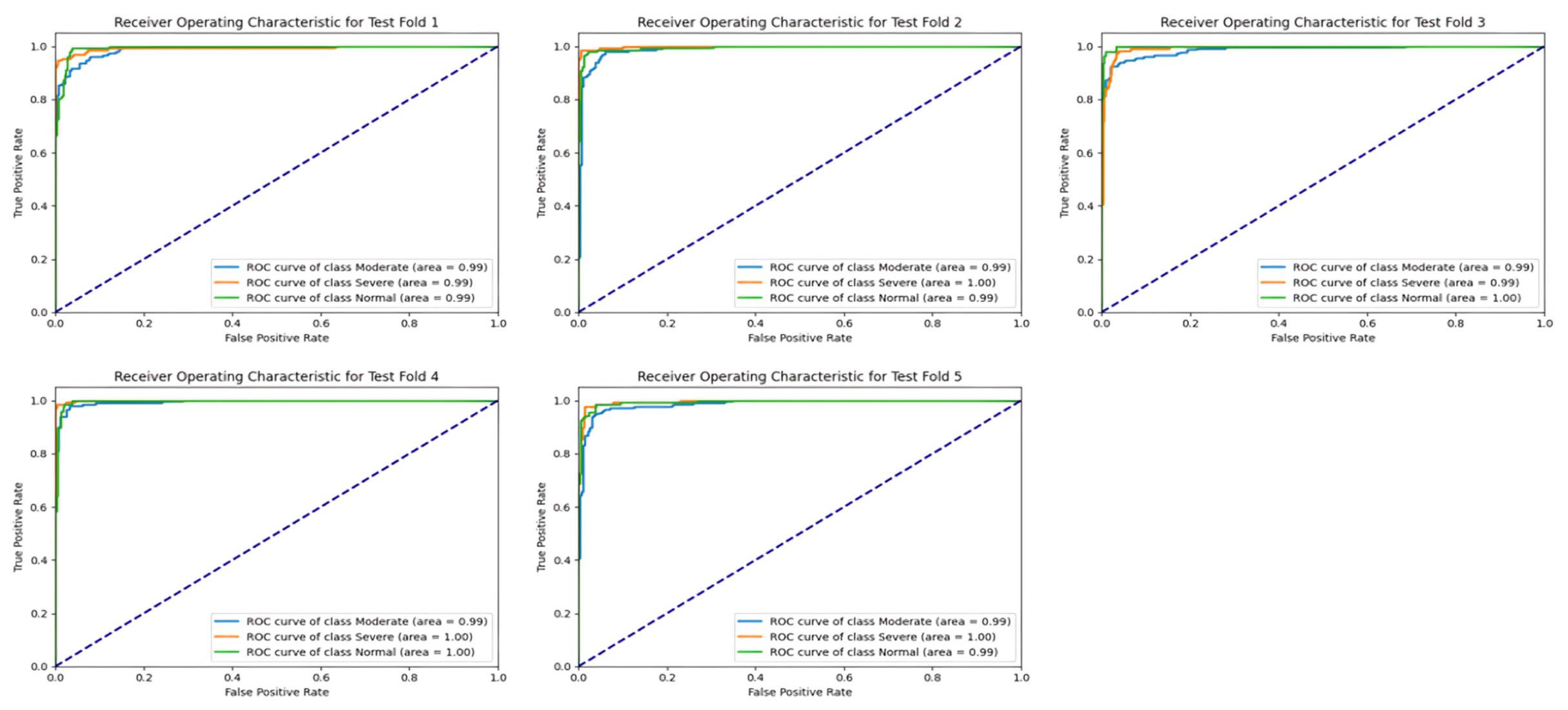
Test
The area under the curve (AUC) values for the test set across different classes and folds demonstrate the consistently high performance of the ResNet-50 model in classification tasks, as shown in
Figure 13. Across all folds, the AUC scores for each class, including Moderate, Severe, and Normal, consistently exceeded 0.98, indicating strong discriminative power and robustness in distinguishing between different severity levels of sinus pathologies. Notably, the Severe class consistently exhibited the highest AUC scores, often surpassing 0.99, suggesting that the model excels particularly in identifying severe cases with high confidence levels. These results underscore the effectiveness of the ResNet-50 model in accurately classifying sinus pathologies based on severity levels.
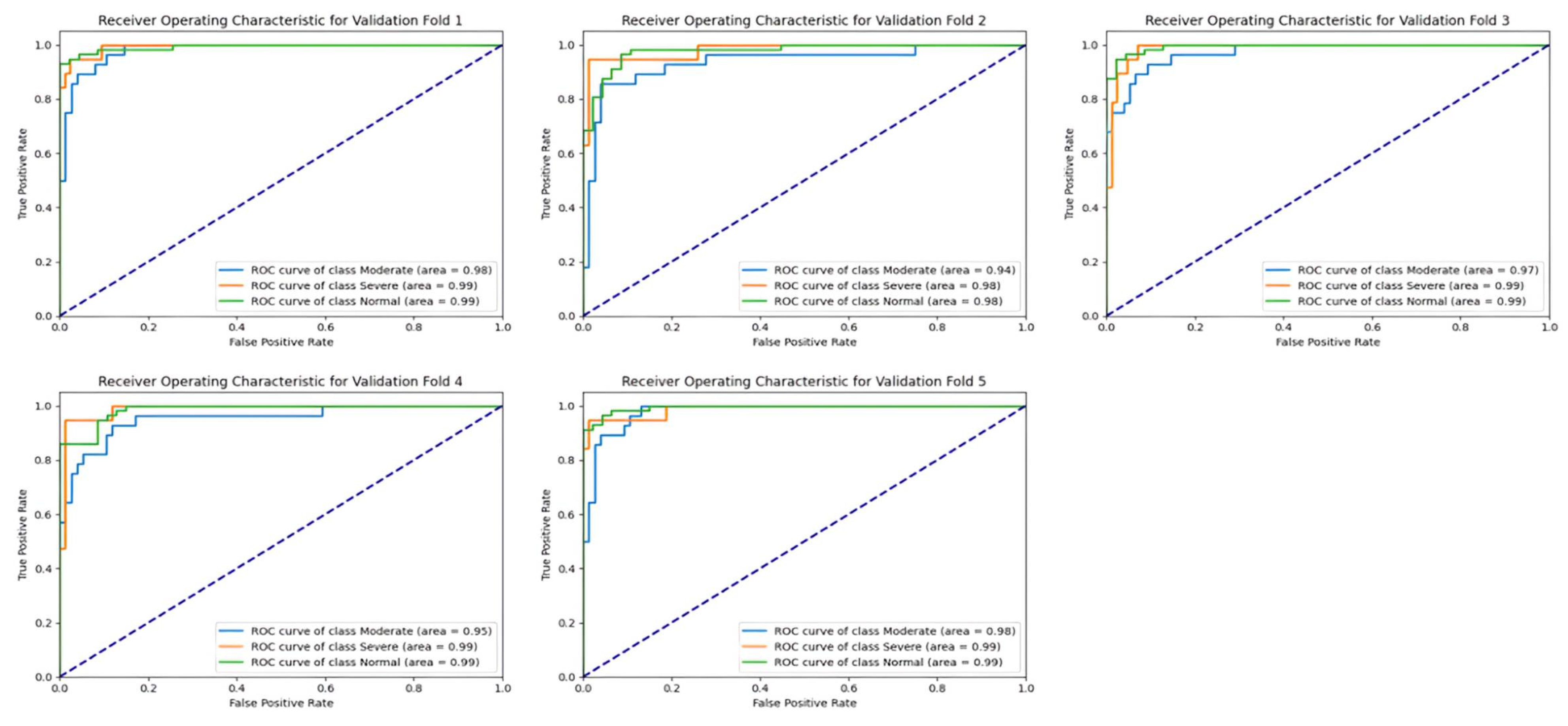
Validation
Similar to the test set, the validation set’s results also demonstrate the strong performance of the ResNet-50 model in terms of AUC values across different classes and folds, as shown in
Figure 14. The AUC scores for each class consistently remained above 0.97, reaffirming the model’s ability to generalize well to unseen data and maintain high discriminative power. Once again, the Severe class exhibited the highest AUC scores, underscoring the model’s proficiency in identifying severe sinus pathologies with high confidence levels. These findings highlight the robustness and reliability of the ResNet-50 model in accurately categorizing sinus pathologies based on severity levels, making it a valuable tool for medical diagnosis and decision-making.
4.5.2. ResNeXt-50
Similar to ResNet-50, the evaluation of the ResNeXt-50 model through Receiver Operating Characteristic (ROC) curves in both the test and validation datasets offers valuable insights into its classification performance across diverse categories of sinus pathologies.
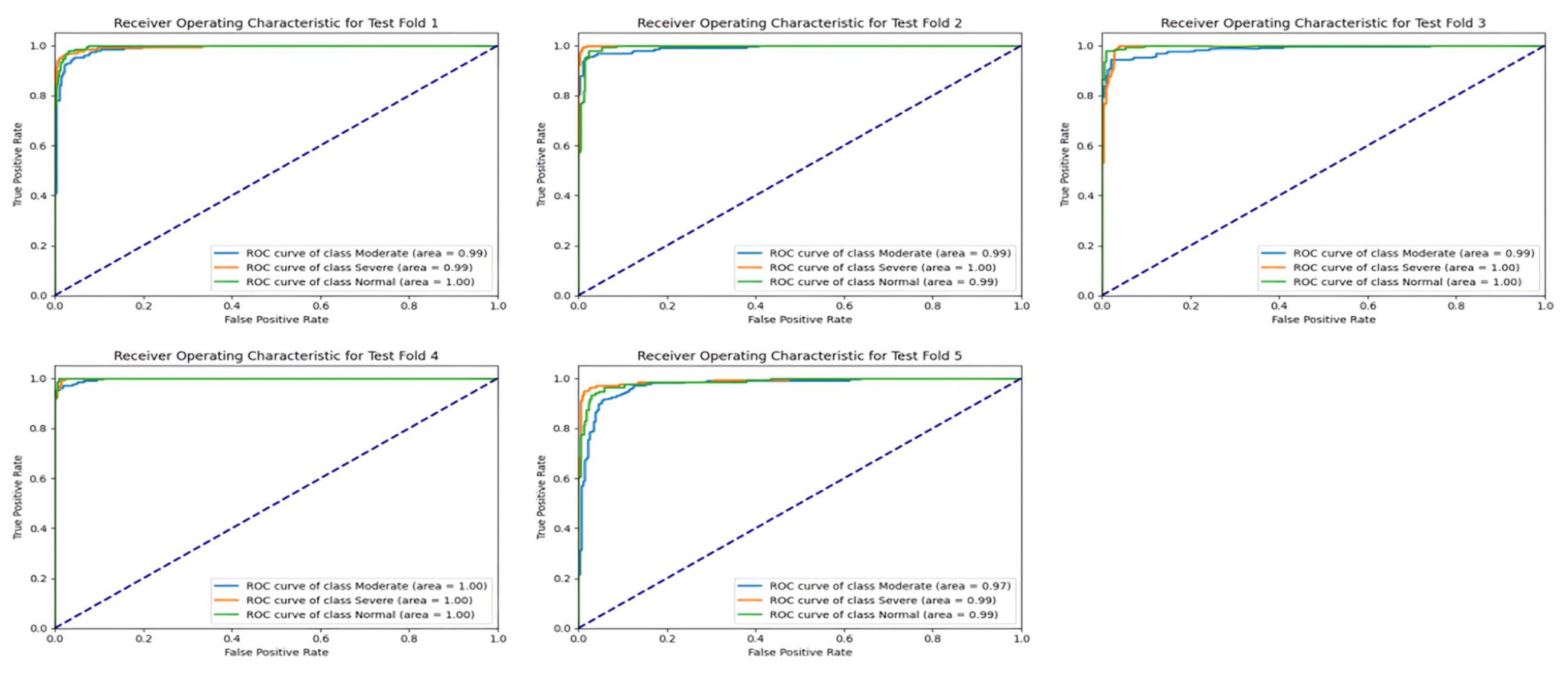
Test
The AUC values for the ResNeXt-50 model in the test set demonstrate consistent and robust performance across different severity classes and folds, as shown in
Figure 15. Across all folds, the AUC scores for each class, including Moderate, Severe, and Normal, consistently exceeded 0.98, indicating strong discriminatory power and reliable classification capabilities. Particularly noteworthy is the consistently high AUC score for the Severe class, often surpassing 0.99, indicating the model’s exceptional ability to accurately identify severe cases with high confidence levels. These results highlight the ResNeXt-50 model’s effectiveness in accurately classifying sinus pathologies based on severity levels, making it a valuable tool for medical diagnosis and decision-making.
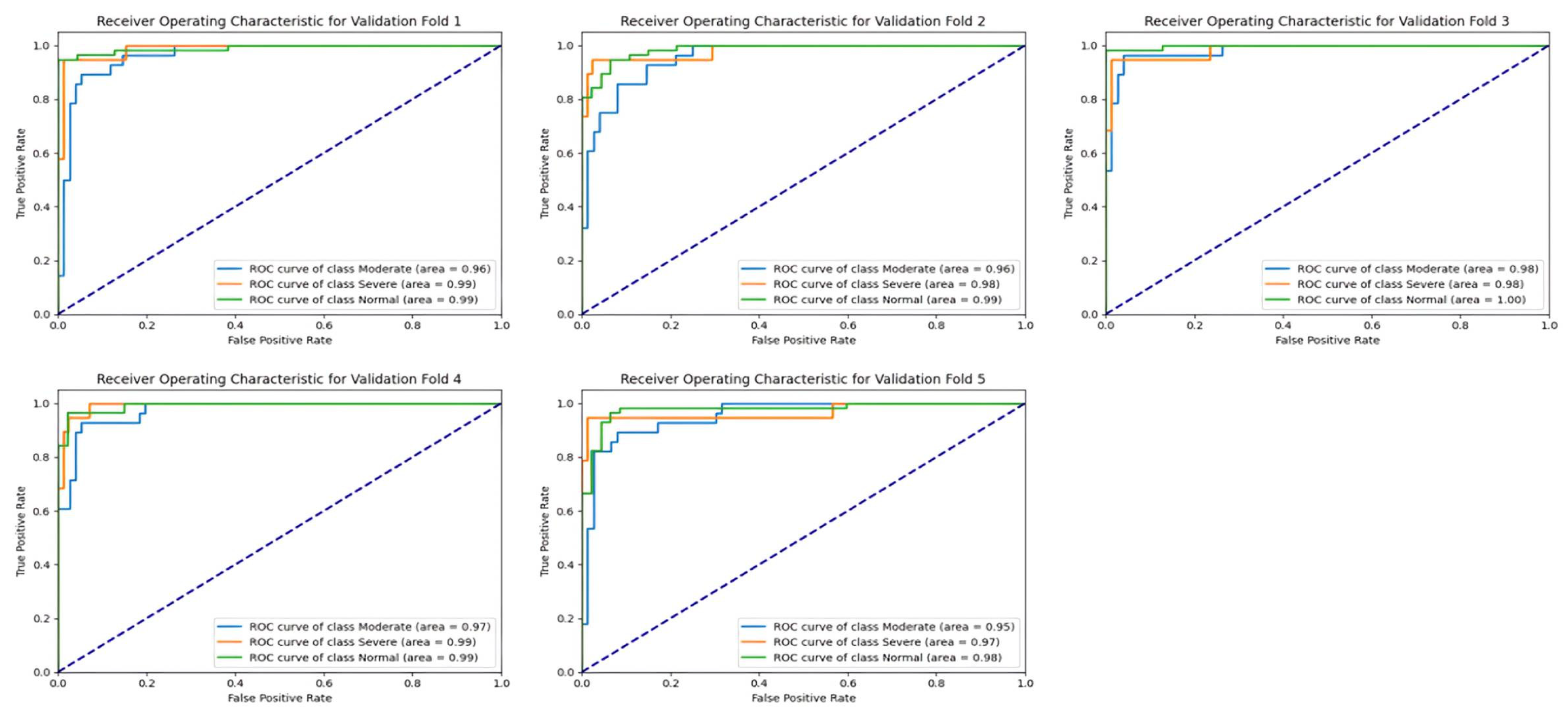
Validation
Similar to the test set, the validation set results also showcase the ResNeXt-50 model’s strong performance in terms of AUC values across different severity classes and folds, as shown in
Figure 16. The AUC scores for each class consistently remained above 0.95, reaffirming the model’s ability to generalize well to unseen data and maintain robust discriminative power. Once again, the Severe class exhibited the highest AUC scores across all folds, indicating the model’s proficiency in identifying severe sinus pathologies with high confidence levels. These findings underscore the ResNeXt-50 model’s reliability and effectiveness in accurately categorizing sinus pathologies based on severity levels, highlighting its utility in clinical applications for diagnosing and managing sinus-related conditions.
5. Conclusions
This work explores the effectiveness of applying GANs to expand datasets and enhance the quality of synthetic images for the training of deep learning models for the detection of sinus pathologies. Employing the lightweight GAN architecture, synthetic images were produced to overcome the challenge of limited training data, specifically for the Moderate and Severe categories. The incorporation of GANs not only increased the diversity and realism of the dataset but also improved the robustness and generalization ability of the classification models. The synthetic images were produced using thorough evaluation and selection processes to make them look as close to the real images as possible. This ensured a close resemblance, which then boosted the performance of the developed deep learning model. ResNeXt-50 was the top-performing model, outperforming ResNet-50 in terms of accuracy and precision in the diagnosis of sinus pathologies. Lastly, this study emphasizes the importance of synthetic data generation techniques for the performance gain in medical image analysis tasks and the use of GANs for diagnostic capabilities’ enhancement in healthcare applications.
Despite the fact that this study has made significant contributions, it is crucial to mention some limitations. One of the limitations is the small dataset size used in this study, which may limit the applicability of the developed deep learning models. Although the attempt to develop a diverse dataset via GAN-based augmentation was made, the size of the original dataset was still small, which may restrict the model’s capability in grasping the full range of variability in sinus diseases. Additionally, the study focused more on Moderate and Severe classes, while the Normal class was overlooked which may impact the model’s performance in detecting the less severe cases. Moreover, while GANs offer a promising approach for synthetic data generation, their effectiveness may vary depending on factors such as model architecture and hyperparameters, introducing variability in the quality of generated images.
Future research can investigate the transferability and scalability of the developed models to different medical imaging modalities or clinical settings. Applying GAN data augmentation methods beyond sinus pathologies to other medical domains can widen the horizon of their application and, consequently, their usefulness in health care. Additionally, understanding the interpretability and explainability of deep learning models when trained on synthetic data is critical in gaining the trust and use of this technology in clinical practice. Incorporating domain knowledge as well as expert input into models and an iterative review in real-world clinical studies are also necessary for realizing the full potential of GANs and deep learning in medical image analysis and diagnosis. Also, future research may also involve leveraging larger datasets to further enhance the robustness and generalization capabilities of the developed deep learning models for sinus-related medical imaging.


