Abstract
Mobile robots play an important role in smart factories, though efficient task assignment and path planning for these robots still present challenges. In this paper, we propose an integrated task- and path-planning approach with precedence constrains in smart factories to solve the problem of reassigning tasks or replanning paths when they are handled separately. Compared to our previous work, we further improve the Regret-based Search Strategy (RSS) for updating the task insertions, which can increase the operational efficiency of machining centers and reduce the time consumption. Moreover, we conduct rigorous experiments in a simulated smart factory with different scales of robots and tasks. For small-scale problems, we conduct a comprehensive performance analysis of our proposed methods and NBS-ISPS, the state-of-the-art method in this field. For large-scale problems, we examine the feasibility of our proposed approach. The results show that our approach takes little computation time, and it can help reduce the idle time of machining centers and make full use of these manufacturing resources to improve the overall operational efficiency of smart factories.
1. Introduction
A smart factory usually has a series of machining centers, industrial robots, storage racks, and mobile robots. The mobile robots can assist the industrial robots and machining centers with complex manufacturing jobs by delivering raw materials and parts and inspecting the status of production lines [1,2,3]. As the number of robots and tasks grows, the scheduling and planning of these robots can become complicated. Therefore, it is necessary to investigate how to efficiently assign and schedule mobile robots to transport materials between machining centers and storage racks with the goal of minimizing the makespan (i.e., the time consumed in transportation and processing) and/or the amount of consumed energy. Moreover, constraints of temporal precedence usually exist between sequential manufacturing processes and material delivery operations (e.g., picking up, delivering, processing, and storing). This type of scheduling and planning problem can be defined as a precedence-constrained multi-agent task assignment and path finding (PC-TAPF) problem [4].
In a PC-TAPF problem, a set of tasks and a team of mobile robots are usually given at the beginning. We first need to assign each task to a suitable robot [5], then a set of conflict-free paths for robots needs to be generated to ensure the assigned tasks can be successfully completed [6,7]. Note that precedence constraints can exist between tasks in a PC-TAPF problem [8]. For example, suppose that A, B, and C are three transportation tasks, and tasks A and task B must be completed before task C is started. Then, the initial position of task C can only be determined once the target positions of task A and task B have been determined in a scenario of flowline production [4]. Therefore, considering that the precedence constraints of transportation tasks are different between these environments, it is not appropriate to simply apply the task assignment and path-planning algorithms developed for warehousing in smart manufacturing.
Various approaches have been developed to solve PC-TAPF problems [9,10,11,12]. These approaches often solve task assignment and path finding separately. The common procedure is to generate all possible assignments, and then, find a feasible path for each assigned task. However, many of these approaches either suffer from high complexity in computation, which leads to difficult deployment in practice, or simply assume the solved paths will not conflict with each other no matter how the tasks are assigned [13,14,15]. For example, Andy Ham [16] proposes a novel application of constraint programming for the job-shop scheduling problem (JSP) with transbots. Fatemi-Anaraki et al. [17] propose mixed-integer linear programming and constraint programming approaches for the scheduling of multi-robot job-shop systems in dynamic environments. These approaches focus on solving task scheduling problems and may not directly apply to those problems where task assignment and path finding are coupled.
In recent years, approaches that jointly solve task assignment and path finding have been emerging. For instance, the CBM (Conflict-Based Min-Cost-Flow) and CBS-TA (Conflict-Based Search with Optimal Task Assignment) algorithms [18,19] can find makespan-optimal solutions to task assignment and path finding. Brown et al. [4] proposed a four-level hierarchical algorithm for computing makespan-optimal solutions to PC-TAPF problems. However, many of these algorithms are limited by poor scalability, and timeout failures can happen when the numbers of agents and tasks become relatively large. In addition, they usually only consider makespan as the single optimization objective.
To tackle these issues, some new methods have been proposed to solve task assignment and path finding problems in an integrated way [20,21,22]. For instance, Dasgupta et al. [20] developed a combined method to generate task sequences by dynamically updating path costs. When the initially calculated paths need to be changed to avoid collisions, their associated task sequences will also be reassigned. Chen et al. [21] designed an integrated method where task assignment choices are determined by actual delivery costs. The actual path cost is considered when assigning tasks to agents for improving the quality of task assignment. However, these methods do not consider the precedence constraints between tasks and may not apply to the scenario of smart manufacturing.
To make up for these shortcomings, in this paper, we propose an integrated task- and path-planning approach for mobile robots in smart factories. This approach can solve task assignment and path planning in a joint way while considering the precedence constraints of tasks and conflict-free constraints of paths. The core ideas of the approach are the Looking-backward Search Strategy (LSS) and Regret-based Search Strategy (RSS) developed for the process of task assignment, which can further reduce the total operating time and the consumed energy of machining centers. Specifically, the Regret-based Search Strategy (RSS) is inspired by the regret mechanism [23,24,25,26] in the task assignment process. In the regret mechanism, instead of greedily choosing the current best solution, both the best and the second-best solutions are considered, which facilitates finding a more efficient solution from a holistic point of view. For example, Zheng et al. [25] used the regret mechanism to assign tasks to mobile robots considering both the smallest and second smallest travel distances. Similarly, Dohn et al. [26] used the idea of regret for determining the weighted sum of the best candidate and second-best candidates to visit each customer in a homecare staff scheduling problem. Our proposed RSS also adopts this mechanism and reduces the idle time of machining centers in smart factories.
Our approach preliminarily solves the coupling of task assignment and path planning while improving the operational efficiency and reducing the energy consumption of the smart factory. It can contribute to the practical deployment of multi-mobile robot systems in smart factories and promote the development of more advanced high-efficiency and energy-saving manufacturing modes.
This paper is structured as follows. Section 2 introduces our integrated task assignment and path-planning approach. Section 3 presents a simulation experiment validating the proposed approach and discusses the experimental results. Section 4 provides a summary of our work and suggests future research directions.
2. Methods
2.1. Problem Formulation
Solving the PC-TAPF problem in a smart manufacturing environment is defined as determining how to optimally assign tasks with precedence constraints and generate conflict-free paths for each moving robot. In our study, the environment is represented as a grid map consisting of cells with a unit length, and an index incrementally numbered from left to right and top to bottom is used as the position coordinate of each cell. For example, in a -cell grid, the cell in the upper left corner is indexed with 0, while that in the lower right corner is indexed with 49. Thus, in path finding, graph-based search methods such as CA* [27] can be adopted.
Let be a set of optional machining centers for task when operating task . This setting considers a scenario where several machining centers are available for a manufacturing job, and generally, the energy consumed by different machining centers and the distance between these machining centers and mobile robots are different, resulting in various total time and energy consumption. For example, to process task , the energy consumption of machining center is , respectively (in most cases ). The time taken to travel to the machining center is , respectively (in most cases, ). In this way, for task , there is coupling between the energy consumed in choosing which machining center to process and the time taken to choose which robot to transport. In fact, the energy consumption is not necessarily smaller when the transportation time is shorter. For example, when and , although the energy consumption of machining center is larger than , it will take less time to transport to machining center compared to . Thus, it is important for a task to choose the proper machining center to save the time and energy. This means that the goal positions of some tasks are unknown before the final task assignment, in which these tasks will eventually be assigned to appropriate machining centers considering both the time and energy efficiency.
Let represent a set of tasks in the smart factory in which the cargo (e.g., materials or parts) is transported from starting positions to designated positions. Each task has a given tuple with seven attributes, . is the type of task , and represents that in task , the cargo will be transported from a storage zone or machining center to another machining center (note here that the goal position of task is still unknown), while represents that the cargo will be transported from a machining center to a storage zone (note here that the goal position of task is known because we assume that the storage location of each part is known and fixed). These constraints are defined in Equations (7)–(9) in the following formulation.
Given a grid map with cells, are the starting and goal positions of task , respectively, which equals −1 when the starting or goal position is unknown. are the starting and finishing times of task , respectively, which equals −1 when either one is unknown. is the parent task of task , and it must be completed before starting task . Here, we only consider a basic case where each task has one parent. represents the set of robots for transporting tasks. denotes the starting position for each robot . The starting positions of all robots are randomly assigned in the docking zone at the beginning. In this study, the robots are assumed to be able to turn around in place; thus, robot heading is not considered in task assignment.
In order to transport task , the initial and goal positions of task need to be determined first through the task assignment process. Then, robot moves to the starting position of the task and transports the cargo to the goal position . During this period, time is set to be discretized into unit time steps, and a robot can move over one cell in one time step. In the path finding process, two types of collisions need to be avoided: vertex collision and edge collision. The former states that two robots should not occupy the same cell at the same time, and the latter means that two robots should not move along adjacent cells in opposite directions at the same time.
Let be all possible positions that robot can arrive at. represents a task assignment mapping table that maps the indices of robot and the loading or unloading position to a fixed value, which equals 0.5 if and only if robot has to reach the position . means that task is assigned to robot . The optimization variable represents a processing mapping table, which equals if and only if the machining center is processing task at time . implies that machining center is idle at time . denotes the number of loading tasks of robot at time . denotes the location of robot at time . denotes the time spent by robot transporting all the tasks assigned to it. and denote the time spent and energy consumed by machining center , respectively, after completing all tasks assigned to it.
The problem formulation is given in Equations (1)–(12). In Equation (1), is the sum of the maximum time spent by all robots transporting all tasks (i.e., , the maximum transportation time), and the maximum time spent by all machining centers to process all tasks (i.e., , the maximum processing time). is the total energy consumed when machining centers are operating, (i.e., , the total processing energy). The weighted sum method is used to convert the multi-objective functions into a single function. and represent the weight of transportation time and processing time, and the weight of energy consumed by machining centers, respectively. The overall optimization goal is to minimize subject to the constraints in Equations (2)–(12).
Minimize
Subject to
Equation (2) indicates that the loading and unloading processes of a task are performed by the same robot. Equation (3) means that a task can only be transported by exactly one robot. Equation (4) implies that each robot is capable of transporting at most one task at a time, i.e., a robot cannot transport multiple tasks simultaneously. Equation (5) implies there is no vertex collisions between robots. Equation (6) implies that there is no edge collision between robots. Equations (7)–(12) describe the constraints of certain task attributes when considering the precedence of tasks, and the details are described below. The time complexity is , where represent the number of optional machining centers, tasks, and robots, is the branching factor of the tree, and is the depth of the goal node.
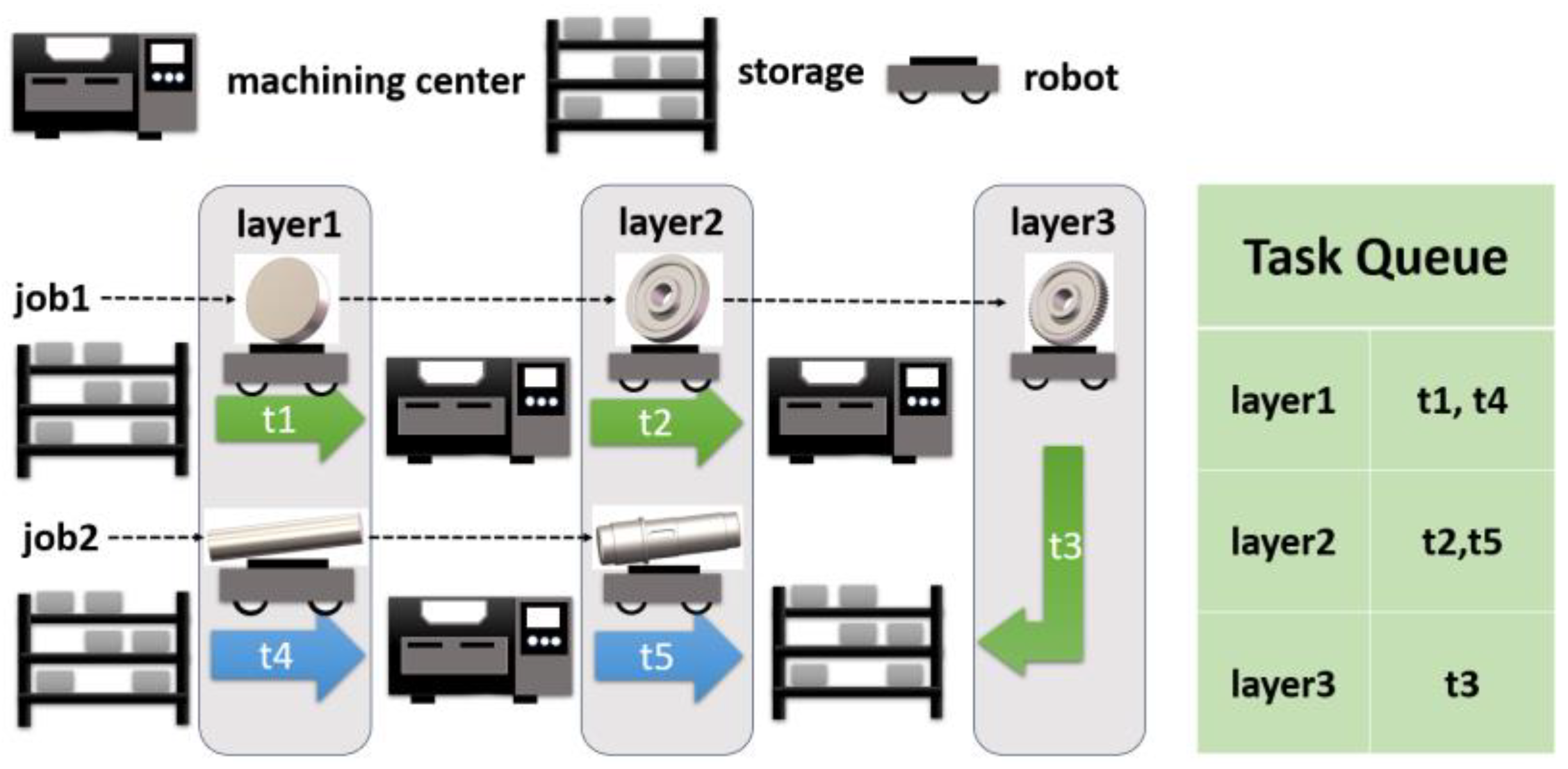
Figure 1 shows an illustrative example of a task queue organized in three layers consisting of five tasks with precedence constraints. represents the manufacturing process of the gear, which can be roughly divided into three tasks—task : machining the outer circle and inner hole, where the robot takes the steel blank from the raw material area and transports it to one of the lathe machines; task : machining the teeth, where the robot transports the workpiece from task to the gear shaping machine; task : warehousing, where the robot transports the workpieces from task to the finished product area. Similarly, represents the manufacturing process of the shaft, which can be roughly divided into two tasks: machining the shaft and warehousing. Obviously, task must be carried out after is completed, while and can be started at the same time. And task is the parent of . In addition, we use to describe the th layer of the task queue, and each layer is a set of tasks in which tasks in the same layer do not need to follow specific sequences, while tasks in two consecutive layers need to be carried out one after another.

Figure 1.
An illustrative example of a task queue organized in three layers consisting of five tasks. and represent the manufacturing processes of the gear and shaft, respectively.
Equations (7) and (8) indicate that the goal position is unknown for task when and is known for task when . This is because the task with needs to select a specific machining center, and its goal position can only be determined after the planning process. The goal position of task with t has to be known so that it can be transported to a designated storage zone. Equation (9) indicates that for all tasks in the base layer (), their starting positions should be known, their starting times are set to 0, their finishing times are unknown initially, and can only be calculated when these tasks are assigned, and all tasks in the base layer are pioneers without parent tasks.
Tasks in () need to be assigned after the completion of their corresponding parent tasks in . This means that the attributes of tasks (e.g., the starting time and the parent task) in are not exactly the same as those in due to the precedence constraints. Equation (10) describes that the starting positions of some tasks are known, while others are unknown. In the latter case, the starting position of the current task depends on the goal position of its corresponding parent task. That is, the starting position of this current task will be known only after its parent task with is assigned. Likewise, Equation (11) requires that a task can be started only after its corresponding parent task is completed. Equation (12) represents a task in that has one parent task when the jobs have not been completed in .
2.2. Integrated Task and Path Planning
Figure 2 shows the overall workflow of the proposed approach. The tasks are first organized into a queue by layer according to their precedence constraints, as shown in Figure 1. Then, tasks are selected from the built task queue in increasing order of precedence layers, i.e., tasks from the base layer are extracted first. For each selected task , process planning is first performed by traversing all available machining centers. For each possible machining center , its position is set as the goal position of task . The energy consumed by the machining center and the machining time can be obtained from the initial settings. Then, CA* is used to generate a reasonable path for robot ensuring that no collision occurs with other planned paths.
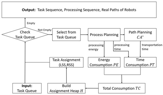
Figure 2.
The overall workflow of the integrated task and path planning approach. CA* [27] is used in the path planning process.
The time consumption and energy consumption for task processing and transportation are taken as the total consumption and stored in the Assignment Heap in increasing order (i.e., the assignment with least total consumption is at the top of the heap). The Assignment Heap contains all potential assignments of task to each available robot and machining center when . The greedy algorithm is then used to select the optimal task assignment from and the loop cycle continues until all tasks are successfully assigned. To reduce unnecessary waiting time for machining centers in the task assignment process, we propose the Looking-backward Search Strategy (LSS) and Regret-based Search Strategy (RSS), which are explained in the following subsections.
2.2.1. Looking-Backward Search Strategy (LSS)
Traditionally, a task will be assigned to a machining center at the time point right after the last task assigned to this machining center is finished. This treatment is named the Baseline method (or the traditional method) in our study, and may lead to unnecessary waiting time since the time periods before starting the last assigned task might be free for inserting the current task. Thus, we propose the Looking-backward Search Strategy (LSS) to reduce the operating time. The basic idea is to search the available time periods before the starting time of the last assigned task (i.e., looking backward) and try to identify whether the current task can fit in any of those time periods.
Algorithm 1 shows the pseudo-code for updating the processing sequence via LSS. denotes the time taken for machining center to process task . denotes the time when robot finishes the transporting task to the machining center , and represents the current total time taken by the machining center to complete the last task that was assigned. Equation (13) describes , the search space of inserting task (i.e., the feasible time periods) when the looking-backward search is performed. Specifically, a counter function count is performed to keep track of the time periods when the machining center is idle. Here the greedy search strategy is used, which means that once we find the first feasible time period insert, the search will stop and the identified period will be the time period for machining center to process task .
| Algorithm 1 | Update Processing Sequence via LSS [28] |
| Input: | current task , robot , machining center |
| Output: | processing mapping table |
| 1: | Initialize |
| 2: | for all do |
| 3: | if then |
| 4: | ++ |
| 5: | if then |
| 6: | for all do |
| 7: | = |
| 8: | end for |
| 9: | end if |
| 10: | end if |
| 11: | if then |
| 12: | |
| 13: | end if |
| 14: | end for |
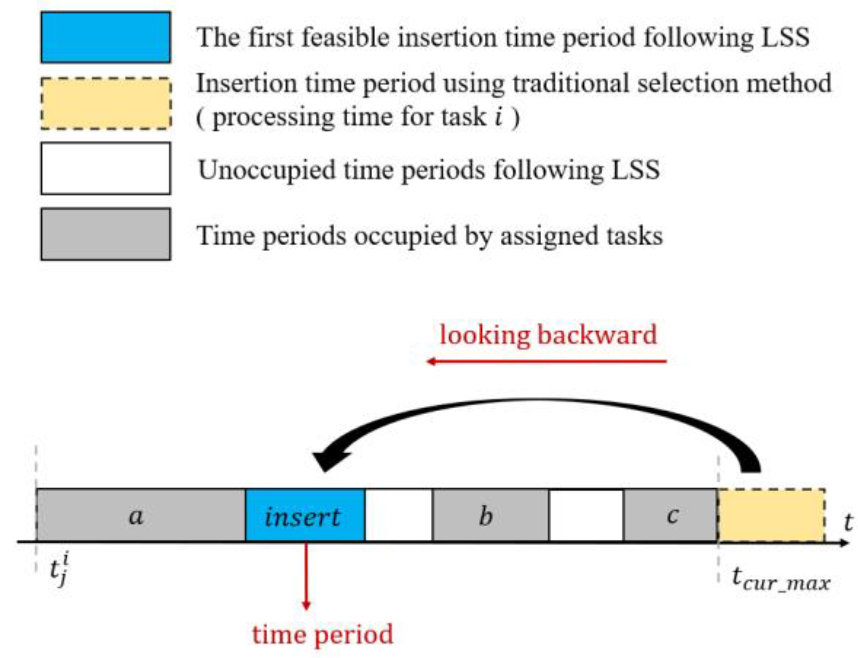
Figure 3 shows an example case of updating the task assignment based on LSS. The gray boxes represent the time periods occupied by assigned tasks (e.g., tasks ) and they cannot be replaced with new tasks. The yellow box represents the insertion time period using the traditional selection method (i.e., the Baseline method). As shown in Figure 3, it is right after the occupied time of the assigned task . In other words, the traditional method does not take into account the idle time of the machining center, but simply adds the needed time period of processing the new task to the end of the machining center’s processing queue. The blue box represents the first feasible insertion time period following LSS, while the white boxes represent unoccupied time periods based on LSS. The search space of the insertion time is . Obviously, the new insertion strategy can reduce the idle time for the machining center, and the total time and energy consumption can be saved.

Figure 3.
An illustration of the Looking-backward Search Strategy (LSS) [28].
2.2.2. Regret-Based Search Strategy (RSS)
Note that LSS will stop searching after finding the first feasible time period for the current task . This greedy strategy may prevent the next task from being inserted backward since the identified time period to process task may partially interfere with the needed time period to process the next task . To address this issue, we propose a Regret-based Search Strategy (RSS). The basic idea is that when we perform the task insertion of the current task , the algorithm also considers leaving enough space for inserting the next task , i.e., thinking one step ahead.
Algorithm 2 shows the pseudo-code for updating the task assignment sequence via RSS. The search space is the same as Equation (13). The core ideas are as follows.
- An array is defined to save all feasible time periods that allow the insertion of task . Note that the time period mentioned in Figure 3 is the same as when the size of is 1.
- Then, the insertion of the next task is considered by filtering out the time periods that allow the insertion of task , which can be accessed by the index .
- Finally, the final time period of task is determinized depending on which of the two cases shown in Figure 4 applies. The details of the two cases are provided as follows.
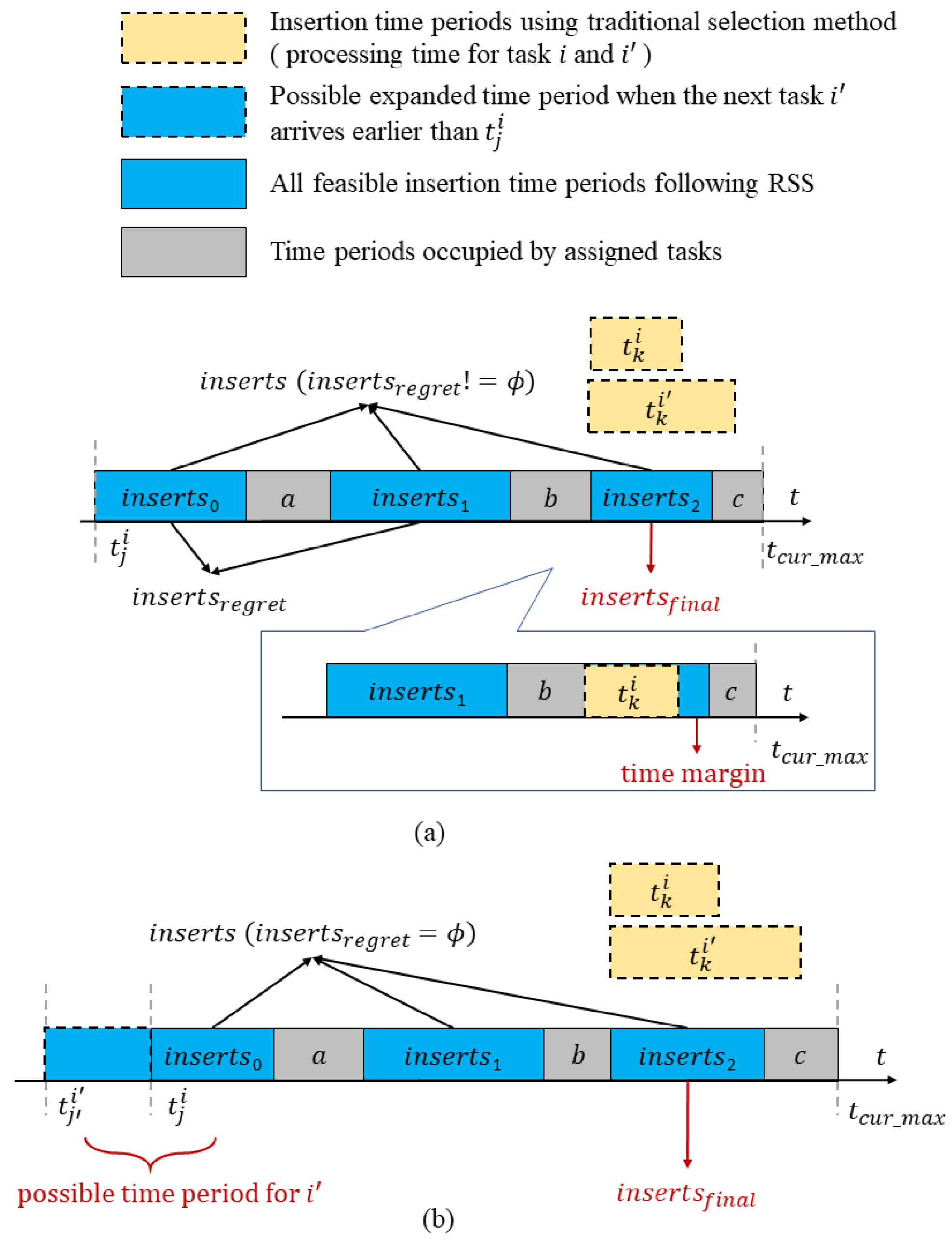
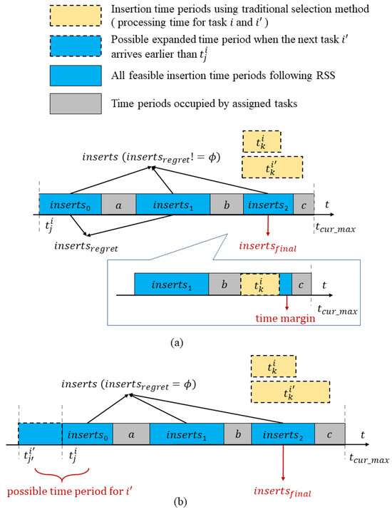 Figure 4. An illustration of the Regret-based Search Strategy (RSS) for the cases when the identified time periods for inserting task (a) allow and (b) do not allow the insertion of the next task [28].
| Algorithm 2 | Update Processing Sequence via RSS [28] |
| Input: | current task , next task , robot , machining center |
| Output: | processing mapping table |
| 1: | Initialize |
| 2: | for all do |
| 3: | Find all feasible time periods of task |
| 4: | end for |
| 5: | //regret |
| 6: | Filter time periods |
| 7: | ifthen |
| 8: | max () |
| 9: | end if |
| 10: | if then |
| 11: | min () |
| 12: | end if |
| 13: | //insert |
| 14: | for all do |
| 15: | |
| 16: | end for |
Figure 4a,b illustrate the RSS method for the cases when the identified time periods for inserting task allow and do not allow the insertion of the next task , respectively. The blue boxes represent the time periods occupied by assigned tasks (e.g., tasks ), and they cannot be replaced with new tasks. The yellow boxes represent the processing time of tasks and . The blue solid boxes represent all feasible insertion time periods following RSS, while the blue dashed box represents the possible expanded time period when the next task arrives earlier than . The search spaces of the insertion times for the current task and the next task are and , respectively. Here, the time margin is defined as the difference between a time period that allows the insertion of a task and the actual needed processing time for that task (i.e., ; see the zoomed-in part of Figure 4a).
In Figure 4a, the array saves all time periods that allow the insertion of task , while stores all time periods that allow the insertion of both tasks and . Then, can be selected following Equation (14). And in Figure 4a, , and will be reserved for the next task . Note that the final insertion time period for task will be assigned in the next loop.
In Figure 4b, we know that . In this case, we will select one from by skipping the time period closest to (i.e., ) and also making its time margin as small as possible (see Equation (15)).
This treatment results from considering if the next task arrives at the machining center earlier than , and the search space of the insertion time for task will expand to . The expanded search space (i.e., the left-side blue dashed box in Figure 4b) and the original search space are likely to form a larger space that may allow the insertion of the next task , and the time consumption can be further reduced. Following the above procedures, the final selected time period for task is , as shown in Figure 4b, and the final insertion time period for task will be assigned in the next loop.
3. Results of Simulation Experiments and Discussion
3.1. Experiment Settings
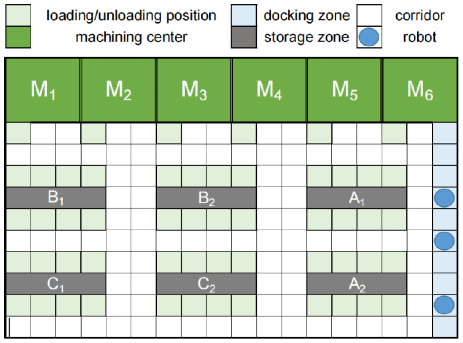
Figure 5 shows the layout of a smart factory represented by a grid map (13 × 18 cells) including machining centers (dark green), corridors (white), docking zones for mobile robots (light blue), and storage zones (dark gray). The storage zones are specified as raw material areas (), semi-finished product areas (), and finished product areas (). The mobile robots (dark blue circles) can perform loading or unloading tasks in the light green cells. After completing all tasks assigned to it, the robot will stop in the docking area to avoid collisions with other robots that are still in working mode.

Figure 5.
Layout of a simulated smart factory [28].
After receiving the starting signal, a mobile robot leaves from the docking area, goes to the raw material area to load the cargo, and transports the cargo to a machining center. Then, the machining center starts to process it. After that, this robot will be assigned to other transport tasks. When the machining center finishes the assigned task, the output (e.g., processed parts) will then be picked up by one of the available robots and transported to another machining center or a shelf in the storage zone. This process will iterate until all tasks are completed.
We examined the performance of our approach in this working scenario with different numbers of robots and tasks. Moreover, we developed a simulation platform in MATLAB R2023a. This platform can visualize the layout of the machining centers, storage zones, and docking zones of the smart factory, and mark out the starting positions and goal positions of all the transportation tasks. It can also dynamically display the moving paths of the robot team to verify the feasibility of the proposed approach (e.g., we can observe whether two robots will collide with each other when performing tasks).
Usually, the quantity of transportation tasks that can be completed per work shift in a smart factory is limited by the processing capability of the machining centers. Therefore, we tested 10 to 1000 tasks in this experiment. The initial positions of mobile robots and the starting and goal positions of tasks are randomly assigned. The assignment of weights reflects the decision maker’s preference for these objectives. In this experiment, we set to 0.6 or 0.4 and . The energy consumed by mobile robots is not considered since it is usually proportional to the transportation time, and is relatively insignificant compared to the energy consumed by machining centers.
3.2. Performance Analysis with Small-Scale Problem
3.2.1. Analysis of Success Rate in Generating Feasible Solutions
We first tested the success rate of the proposed approach with small-scale problems. Here, the success rate is defined as the number of experiments with feasible solutions for task assignment and the path plans generated divided by the total number of experiments tested. A total of 20 sets of experiments with the quantity of tasks varying from 10 to 100 and with 5 or 10 robots were generated. The time spent and energy consumed by machining centers for each task were randomly set as constants.
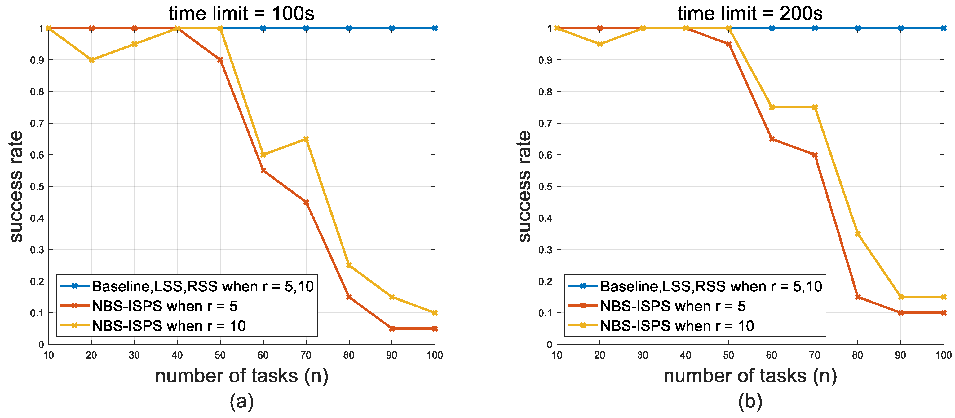
Figure 6 shows the relationship between success rate and the number of tasks with different numbers of robots and time limits when comparing our proposed methods with a popular method for PC-TAPF problems: Sequential Next-Best Assignment Search-Incremental Slack-Prioritized Search (NBS-ISPS) [4]. In NBS-ISPS, task assignment and path planning were solved by the NBS solver and ISPS solver, respectively, and independently. The time limit means the maximum allowed runtime of the optimization solver in NBS-ISPS.
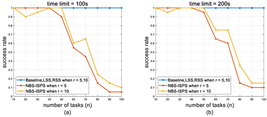
Figure 6.
The relationship between success rate and the number of tasks () for our methods and the NBS-ISPS method with different numbers of robots () and time limits: (a) time limit = 100 s; (b) time limit = 200 s.
Figure 6 indicates that the success rate of our proposed methods is 100%, while the success rate of the NBS-ISPS method decreases with an increasing number of tasks, which implies that the NBS-ISPS method may not be suitable for large-scale problems. When the number of tasks is , the success rate seems to be mainly influenced by path planning, since the ISPS solver sometimes cannot generate feasible solutions within a finite number of iterations and sometimes reaches no solution. Thus, the ISPS solver itself is incomplete. When , the success rate is mainly affected by task assignment. In this case, the number of tasks is much larger than the number of robots , and the NBS solver may not be able to find a feasible solution in finite time. For example, in Figure 6a, when , the success rate of NBS-ISPS is only 15%.
By comparing Figure 6a,b, we find that increasing the time limit within a certain range can improve the success rate of NBS-ISPS. For example, when , and the time limit is 100 s or 200 s, the success rate of NBS-ISPS is 90% or 95%, respectively. Furthermore, we examined the effects of different numbers of robots on the success rate, and found that the success rate of NBS-ISPS grows as the number of robots increases. In summary, our proposed methods outperform the NBS-ISPS method in terms of success rate with small-scale problems.
3.2.2. Analysis of Average Time Consumption
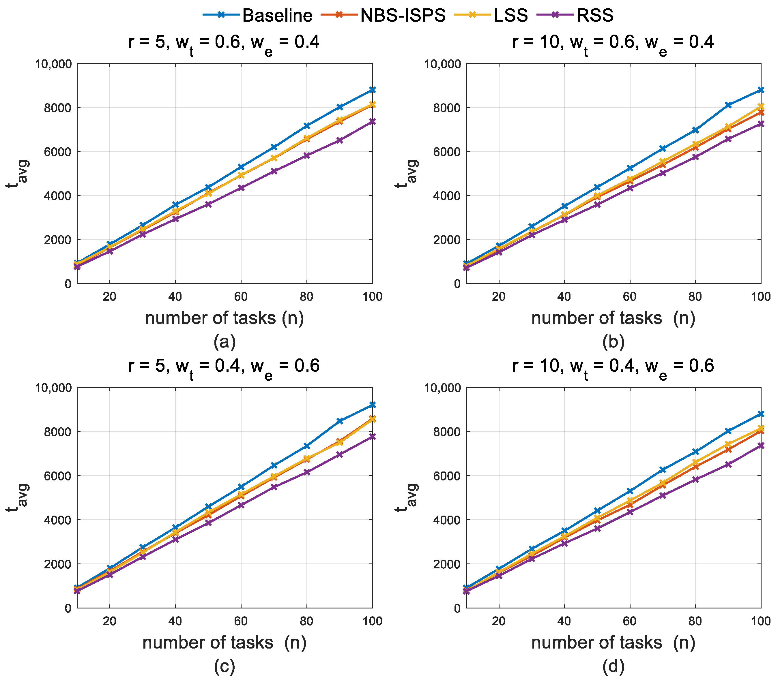
Figure 7 shows the average time consumption () for the whole transportation and manufacturing process in 20 sets of experiments using our proposed methods and the NBS-ISPS method with different numbers of tasks and robots and varying weights. Baseline means a task will be assigned to a machining center at the time point right after the last task assigned to this machining center is finished.
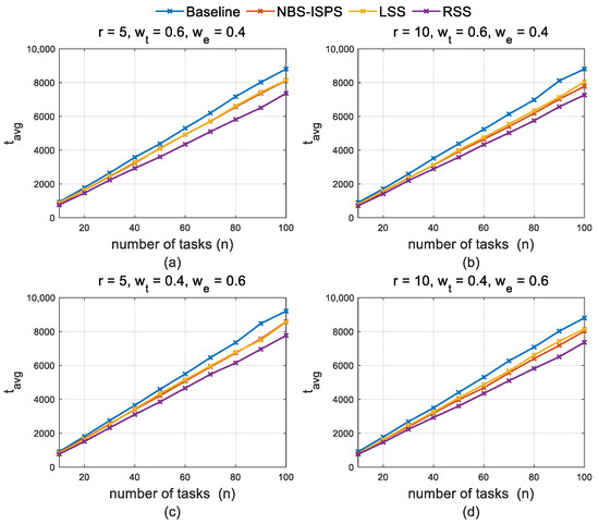
Figure 7.
The relationship between average time consumption () and number of tasks () for our methods and the NBS-ISPS method with different numbers of robots (), the weight of time consumption (), and the weight of energy consumption (): (a) ; (b) ; (c) ; (d) .
Figure 7 indicates that the average time consumption of the proposed LSS method is close to that of the NBS-ISPS method. The RSS method performs better than the NBS-ISPS method, and the Baseline method performs the worst. This is potentially because the RSS method tries to reduce the total time consumption by reorganizing the processing sequences of machining centers, while the NBS-ISPS method does not more effectively account for the time consumed by machining centers. Usually, the time consumed in smart factories concentrates on the processing of workpieces and parts, while the time spent transporting materials accounts for a relatively smaller proportion of the total time consumption. Therefore, the NBS-ISPS method may not be applicable when the time consumed by machining centers is a main concern.
3.2.3. Runtime Analysis
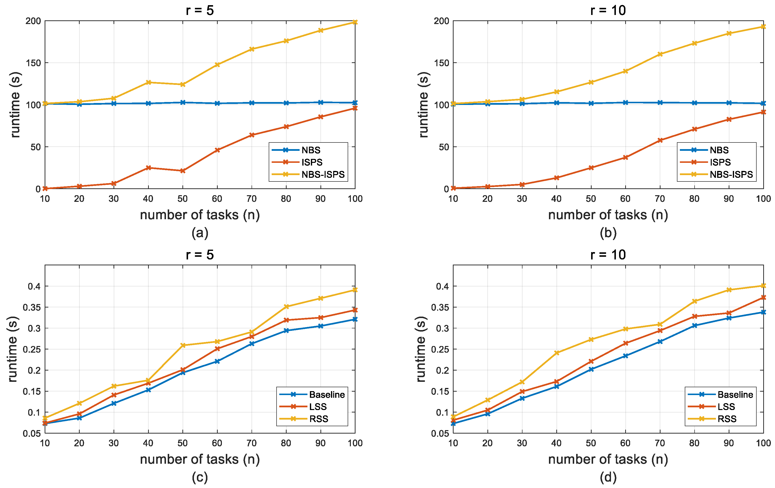
Figure 8 shows the relationship between the runtime of the NBS-ISPS method (when time limit = 100 s) and our proposed methods with different numbers of tasks and robots. In Figure 8a, we can find that the runtime of the task assignment (NBS solver) always exceeds the time limit, which means that the task assignment can hardly find optimal solutions within 100 s. In addition, the runtime of the NBS-ISPS method generally grows as the number of tasks increases. When the number of robots increases from 5 to 10, the runtime of these methods does not change too much.
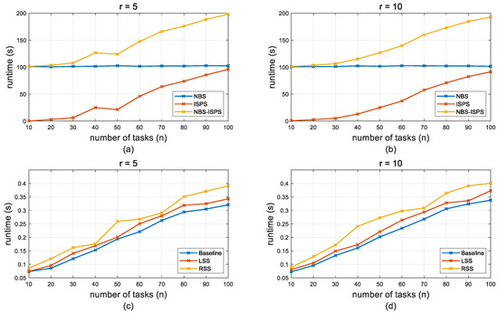
Figure 8.
The relationship between runtime and number of tasks () for our methods and the NBS-ISPS method with different numbers of robots (): (a,c) ; (b,d) . The time limit for the NBS-ISPS method is 100 s.
By comparing Figure 8a vs. Figure 8c or Figure 8b vs. Figure 8d, we find that the NBS-ISPS method consumes a significant amount of time, while our proposed methods only require a very small runtime. For example, when , the runtime of NBS-ISPS is 147.623 s and the runtime of RSS is only 0.254 s. In real manufacturing conditions, the runtime for the NBS-ISPS method is almost unbearable. This result also reveals the practical value of our methods.
3.3. Feasibility Analysis with Large-Scale Problems
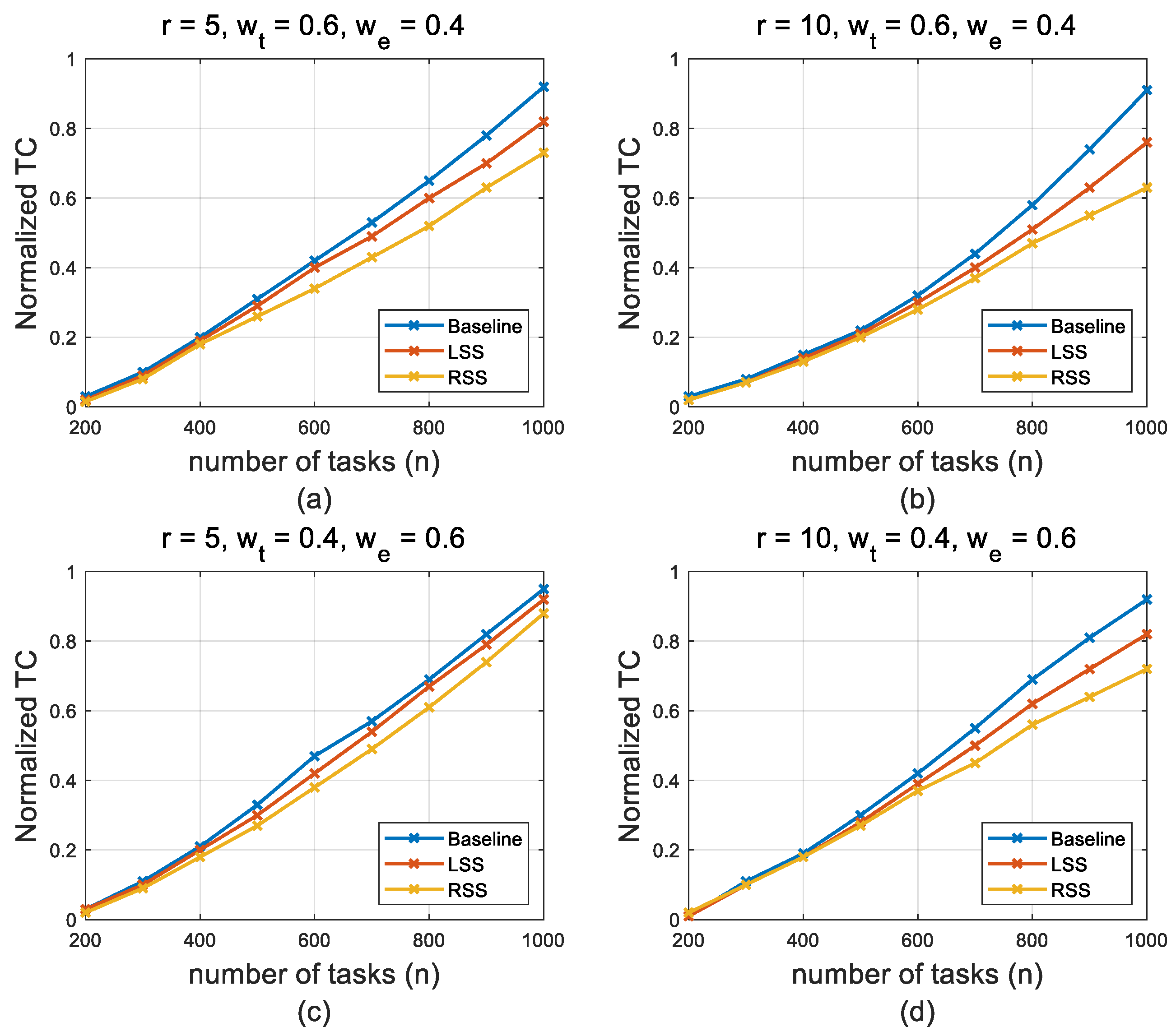
Finally, we examined the feasibility of our proposed approach by comparing the total time and energy consumption of three methods with large-scale problems (200–1000 tasks), as shown in Figure 9. Since the NBS-ISPS method cannot successfully generate solutions for large-scale problems (even with an allowed runtime of more than 1000 s), it is not included in this figure. Here, the total time and energy consumption () are normalized following Equation (16):
where is the time and energy consumed for transportation and processing, and and are the maximum and minimum sum of time or energy consumed for transporting and processing.
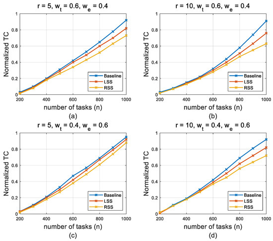
Figure 9.
The relationship between normalized total consumption () and number of tasks () for our proposed methods with different numbers of robots (), weight of time consumption (), and weight of energy consumption (): (a) ; (b) ; (c) ; (d) .
Figure 9 shows that the total time and energy consumption grow with the number of tasks, and the RSS method performs better than the LSS method. Both RSS and LSS outperform the Baseline method for a varying number of robots and tasks.
By comparing Figure 9a vs. Figure 9b and Figure 9c vs. Figure 9d, we can see that when the Baseline method is adopted, increasing the number of robots will not significantly reduce the total consumption. For example, when using the Baseline method and , the normalized values in Figure 9a,b are 0.923 and 0.911, respectively. However, the total consumption decreases markedly if the LSS or RSS method is used. When using LSS with , the normalized values in Figure 9a,b are 0.819 and 0.761, respectively. One possible explanation is that when the processing time and energy consumption of machining centers are not considered (e.g., in warehousing and logistics scenarios), more robots will support the faster completion of tasks. However, when the processing time and energy consumption of machining centers are considered (e.g., in a smart factory environment), even if the number of robots increases and the tasks can be transported to machining centers faster, it still takes a certain amount of time for machining centers to process these tasks. This leads to the queuing of tasks and waiting of robots, and the total time consumption will not be significantly reduced. However, the LSS or RSS method can reorganize the processing sequence of tasks in real time, which can alleviate the queuing issue and reduce the waiting time for robots. Thus, the decrease in will be more obvious when the LSS or RSS method is adopted.
In addition, by comparing Figure 9a vs. Figure 9c and Figure 9b vs. Figure 9d, we can observe the influence of different weights of time and energy on the final . For example, if using RSS with , the normalized , while when , the normalized . This result indicates that the advantage of RSS method is more pronounced when the weight of time () is larger. A possible explanation is that the search of the machining sequence is performed only after each determination of which machining center is assigned, i.e., the energy consumption does not vary with the insertion position since we only consider the time consumed by the machining center without considering the energy consumption during its idle time.
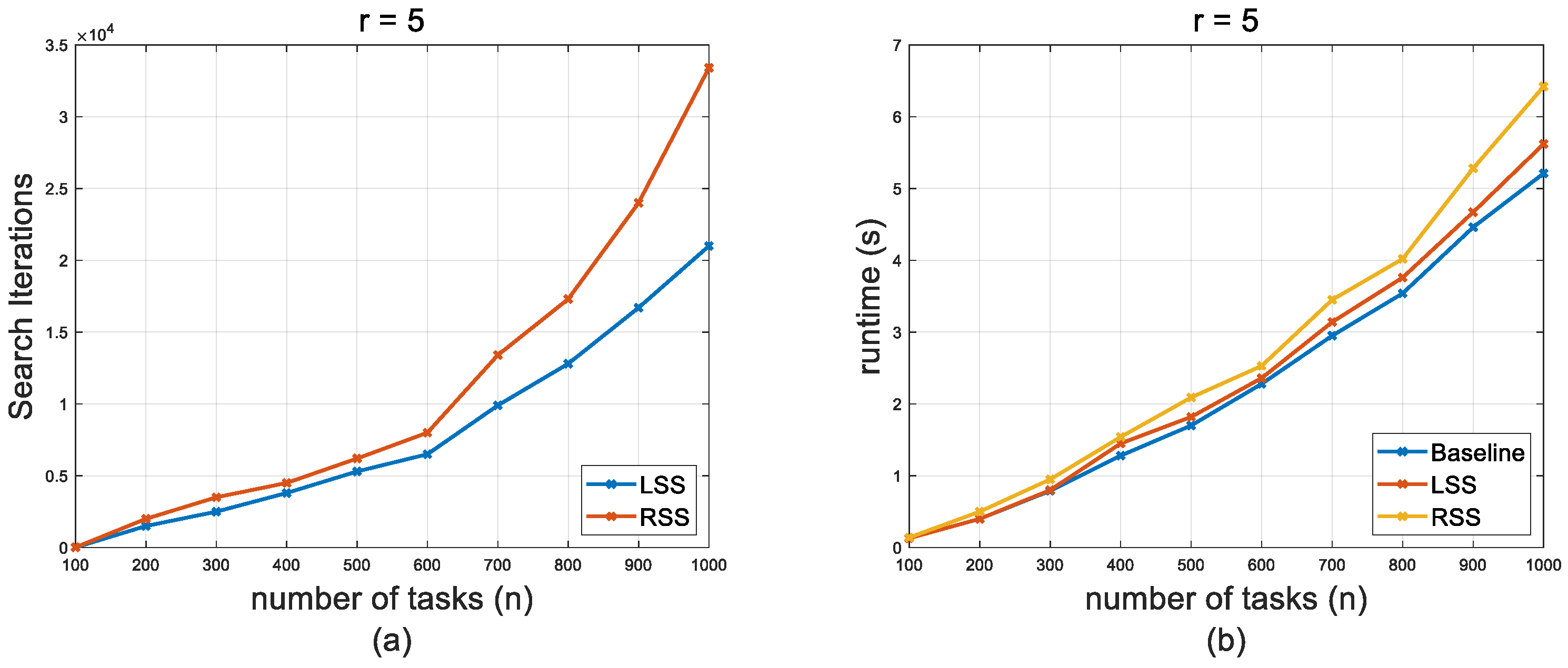
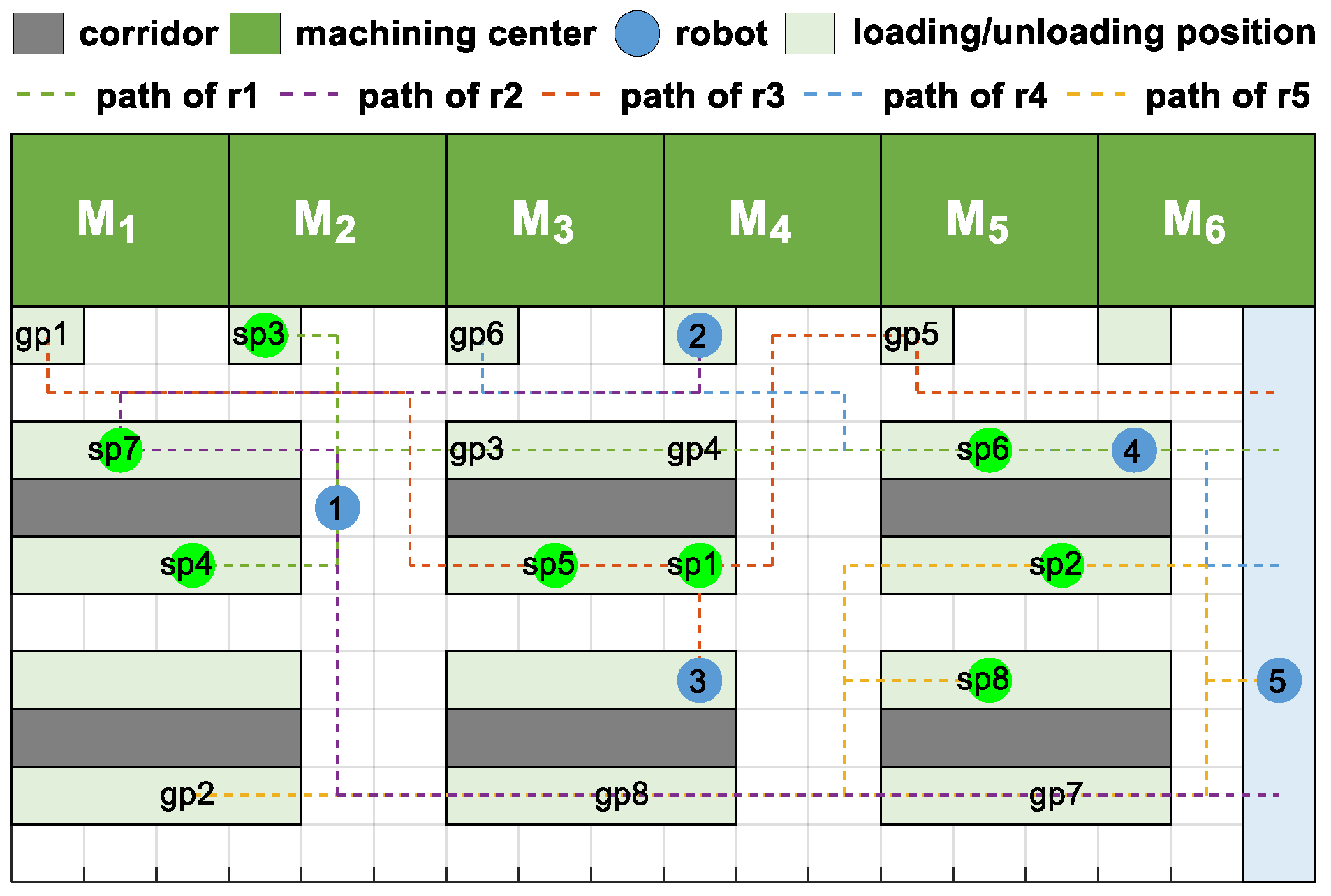
Figure 10 shows the number of searching iterations and runtime of the proposed methods versus the number of tasks with large-scale problems. Figure 10a indicates that the number of search iterations increases along with the increasing number of tasks. The number of search iterations using the RSS method is greater than that using the LSS method, which can lead to slightly longer computation time, as shown in Figure 10b. We also checked the generated paths of each robot in a simulation environment developed with MATLAB 2023a, as shown in Figure 11, and no conflicting paths are found.
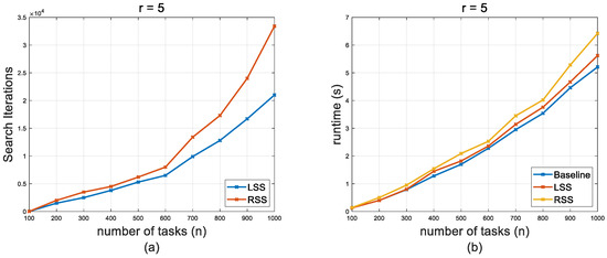
Figure 10.
Computational efficiency of proposed methods with 5 robots for large-scale problems: (a) relationship between number of search iterations and number of tasks (); (b) relationship between runtime and number of tasks (). The Baseline method is not included in (a) because it does not utilize any searching strategy for assigning tasks, i.e., no search iterations are involved.
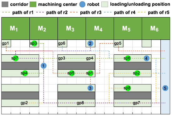
Figure 11.
A simulation environment developed in MATLAB 2023a to verify the feasibility of generated paths for mobile robots [28]. The numbers in blue circles and green circles are the indices of robots and start positions of transportation tasks, respectively.
4. Conclusions
In this paper, we present an integrated task- and path-planning approach for mobile robots in a smart factory. The basic idea is that in the stage of task assignment, the real paths for mobile robots are identified and the time and energy consumed by mobile robots and machining centers are calculated. Then, a greedy strategy in conjunction with the Looking-backward Search Strategy or Regret-based Search Strategy is used to obtain task assignments in time series that satisfy the proposed objectives, which enables a joint efficient solution to be established for both task assignment and path planning. The real time consumed on the planned paths is used as the basis to adjust and improve the selection of mobile robots and task assignments, and the precedence constraints between sequential manufacturing tasks are considered simultaneously.
The performance of our proposed methods is compared with NBS-ISPS, a popular method for PC-TAPF problems in a simulated factory environment with small-scale problems. The results show that the success rate of the proposed methods outperforms that of the NBS-ISPS method, and the average time consumption of the proposed methods is close to that of the NBS-ISPS method. Moreover, our proposed methods run much faster than NBS-ISPS, which allows smoother deployment of these methods in real-world scenarios.
We also analyze the feasibility of our proposed methods with large-scale problems. The results show that the proposed LSS method and RSS method are better than the traditional method (Baseline) when the number of tasks or robots increases, especially when the number of tasks is large. In addition, when the weight of time consumption increases, the advantage of our approach becomes more noticeable. The proposed approach generally requires a short computation time, and it can help reduce the idle time of machining centers and make full use of these resources to improve the overall operational efficiency of smart factories.
One limitation of this study is that the size of the studied factory is relatively small. We will examine the reliability and computational efficiency of the proposed approach in a large-scale factory environment where the planning and scheduling of transportation tasks for mobile robots can be more difficult. The complex relationship between manufacturing time and consumed energy will also be considered in future work.
Author Contributions
Conceptualization, S.L., Y.B., B.F. and D.Y.; methodology, S.L.; formal analysis, S.L., Y.B., B.F. and D.Y.; data curation, S.L.; writing—original draft preparation, S.L. and B.F.; writing—review and editing, Y.B.; funding acquisition, Y.B. All authors have read and agreed to the published version of the manuscript.
Funding
This research was funded by the National Key R&D Program of China (2022YFB4702400).
Institutional Review Board Statement
Not applicable.
Informed Consent Statement
Not applicable.
Data Availability Statement
The data supporting the conclusions of this article will be made available by the authors upon request.
Conflicts of Interest
The authors declare no conflicts of interest.
References
- Yadav, A.; Jayswal, S.C. Modelling of Flexible Manufacturing System: A Review. Int. J. Prod. Res. 2018, 56, 2464–2487. [Google Scholar] [CrossRef]
- Bogue, R. The Changing Face of the Automotive Robotics Industry. Ind. Robot Int. J. Robot. Res. Appl. 2022, 49, 386–390. [Google Scholar] [CrossRef]
- Bogue, R. The Role of Robots in the Electronics Industry. Ind. Robot Int. J. Robot. Res. Appl. 2023, 50, 717–721. [Google Scholar] [CrossRef]
- Brown, K.; Peltzer, O.; Sehr, M.A.; Schwager, M.; Kochenderfer, M.J. Optimal Sequential Task Assignment and Path Finding for Multi-Agent Robotic Assembly Planning. In Proceedings of the 2020 IEEE International Conference on Robotics and Automation (ICRA), Paris, France, 31 May–31 August 2020; pp. 441–447. [Google Scholar]
- Saravanan, S.; Ramanathan, K.C.; MM, R.; Janardhanan, M.N. Review on State-of-the-Art Dynamic Task Allocation Strategies for Multiple-Robot Systems. Ind. Rob. 2020, 110, 52. [Google Scholar] [CrossRef]
- Lai, X.; Li, J.; Chambers, J. Enhanced Center Constraint Weighted A* Algorithm for Path Planning of Petrochemical Inspection Robot. J. Intell. Robot. Syst. 2021, 102, 78. [Google Scholar] [CrossRef]
- Stern, R. Multi-Agent Path Finding—An Overview. In Artificial Intelligence; Springer: Berlin/Heidelberg, Germany, 2019; pp. 96–115. [Google Scholar]
- Korsah, G.A.; Stentz, A.; Dias, M.B. A Comprehensive Taxonomy for Multi-Robot Task Allocation. Int. J. Rob. Res. 2013, 32, 1495–1512. [Google Scholar] [CrossRef]
- Bredstrom, D.; Rönnqvist, M. A Branch and Price Algorithm for the Combined Vehicle Routing and Scheduling Problem with Synchronization Constraints. NHH Department of Finance & Management Science Discussion Paper No. 2007/7. Available online: https://ssrn.com/abstract=971726 (accessed on 24 January 2024).
- Yu, J.; LaValle, S.M. Multi-Agent Path Planning and Network Flow. In Algorithmic Foundations of Robotics X; Springer: Berlin/Heidelberg, Germany, 2013; pp. 157–173. [Google Scholar]
- Yu, J.; LaValle, S.M. Optimal Multi-Robot Path Planning on Graphs: Structure and Computational Complexity. arXiv 2015, arXiv:1507.03289. [Google Scholar]
- Ma, H.; Wagner, G.; Felner, A.; Li, J.; Kumar, T.K.; Koenig, S. Multi-Agent Path Finding with Deadlines. arXiv 2018, arXiv:1806.04216. [Google Scholar]
- Bennewitz, M.; Burgard, W.; Thrun, S. Finding and Optimizing Solvable Priority Schemes for Decoupled Path Planning Techniques for Teams of Mobile Robots. Rob. Auton. Syst. 2002, 41, 89–99. [Google Scholar] [CrossRef]
- Erdem, E.; Kisa, D.G.; Oztok, U.; Schüller, P. A General Formal Framework for Pathfinding Problems with Multiple Agents. In Proceedings of the Twenty-Seventh AAAI Conference on Artificial Intelligence, Bellevue, WA, USA, 14–18 July 2013. [Google Scholar]
- Dai, M.; Tang, D.; Giret, A.; Salido, M.A. Multi-Objective Optimization for Energy-Efficient Flexible Job Shop Scheduling Problem with Transportation Constraints. Robot. Comput. Integr. Manuf. 2019, 59, 143–157. [Google Scholar] [CrossRef]
- Ham, A. Transfer-Robot Task Scheduling in Job Shop. Int. J. Prod. Res. 2021, 59, 813–823. [Google Scholar] [CrossRef]
- Fatemi-Anaraki, S.; Tavakkoli-Moghaddam, R.; Foumani, M.; Vahedi-Nouri, B. Scheduling of Multi-Robot Job Shop Systems in Dynamic Environments: Mixed-Integer Linear Programming and Constraint Programming Approaches. Omega 2023, 115, 102770. [Google Scholar] [CrossRef]
- Sharon, G.; Stern, R.; Felner, A.; Sturtevant, N.R. Conflict-Based Search for Optimal Multi-Agent Pathfinding. Artif. Intell. 2015, 219, 40–66. [Google Scholar] [CrossRef]
- Hönig, W.; Kiesel, S.; Tinka, A.; Durham, J.; Ayanian, N. Conflict-Based Search with Optimal Task Assignment. In Proceedings of the International Joint Conference on Autonomous Agents and Multiagent Systems, Stockholm, Sweden, 10–15 July 2018. [Google Scholar]
- Dasgupta, P.; Woosley, B. Multirobot Task Allocation with Real-Time Path Planning. In Proceedings of the Florida AI Research Society, St. Pete Beach, FL, USA, 22–24 May 2013. [Google Scholar]
- Chen, Z.; Alonso-Mora, J.; Bai, X.; Harabor, D.D.; Stuckey, P.J. Integrated Task Assignment and Path Planning for Capacitated Multi-Agent Pickup and Delivery. IEEE Robot. Autom. Lett. 2021, 6, 5816–5823. [Google Scholar] [CrossRef]
- Elfakharany, A.; Ismail, Z.H. End-to-End Deep Reinforcement Learning for Decentralized Task Allocation and Navigation for a Multi-Robot System. Appl. Sci. 2021, 11, 2895. [Google Scholar] [CrossRef]
- Tillman, F.A.; Cain, T.M. An Upperbound Algorithm for the Single and Multiple Terminal Delivery Problem. Manag. Sci. 1972, 18, 664–682. [Google Scholar] [CrossRef]
- Diana, M.; Dessouky, M.M. A New Regret Insertion Heuristic for Solving Large-Scale Dial-a-Ride Problems with Time Windows. Transp. Res. Part B Methodol. 2004, 38, 539–557. [Google Scholar] [CrossRef]
- Zheng, S.K.X.; Tovey, C.; Borie, R.; Kilby, P.; Markakis, V.; Keskinocak, P. Agent Coordination with Regret Clearing. In Proceedings of the AAAI Conference on Artificial Intelligence, Chicago, IL, USA, 13–17 July 2008; AAAI Press: Palo Alto, CA, USA, 2008; p. 101. [Google Scholar]
- Dohn, A.; Rasmussen, M.S.; Larsen, J. The Vehicle Routing Problem with Time Windows and Temporal Dependencies. Networks 2011, 58, 273–289. [Google Scholar] [CrossRef]
- Silver, D. Cooperative Pathfinding. In Proceedings of the AAAI Conference on Artificial Intelligence and Interactive Digital Entertainment, Marina Del Rey, CA, USA, 1–2 June 2005; Volume 1, pp. 117–122. [Google Scholar]
- Liu, S.; Feng, B.; Yu, D.; Bi, Y. An Integrated Task and Path Planning Approach for Mobile Robots in Smart Factory. In Proceedings of the ASME International Mechanical Engineering Congress and Exposition, Columbus, OH, USA, 30 October–3 November 2022; ASME: New York, NY, USA, 2022; Volume 2B, p. V02BT02A058. [Google Scholar]

Disclaimer/Publisher’s Note: The statements, opinions and data contained in all publications are solely those of the individual author(s) and contributor(s) and not of MDPI and/or the editor(s). MDPI and/or the editor(s) disclaim responsibility for any injury to people or property resulting from any ideas, methods, instructions or products referred to in the content. |
© 2024 by the authors. Licensee MDPI, Basel, Switzerland. This article is an open access article distributed under the terms and conditions of the Creative Commons Attribution (CC BY) license (https://creativecommons.org/licenses/by/4.0/).