A Multi-Objective Optimal Control Method for Navigating Connected and Automated Vehicles at Signalized Intersections Based on Reinforcement Learning

Abstract

The emergence and application of connected and automated vehicles (CAVs) have played a positive role in improving the efficiency of urban transportation and achieving sustainable development. To improve the traffic efficiency at signalized intersections in a connected environment while simultaneously reducing energy consumption and ensuring a more comfortable driving experience, this study investigates a flexible and real-time control method to navigate the CAVs at signalized intersections utilizing reinforcement learning (RL). Initially, control of CAVs at intersections is formulated as a Markov Decision Process (MDP) based on the vehicles’ motion state and the intersection environment. Subsequently, a comprehensive reward function is formulated considering energy consumption, efficiency, comfort, and safety. Then, based on the established environment and the twin delayed deep deterministic policy gradient (TD3) algorithm, a control algorithm for CAVs is designed. Finally, a simulation study is conducted using SUMO, with Lankershim Boulevard as the research scenario. Results indicate that the proposed methods yield a 13.77% reduction in energy consumption and a notable 18.26% decrease in travel time. Vehicles controlled by the proposed method also exhibit smoother driving trajectories.

1. Introduction

Optimizing traffic at intersections, a pivotal node within the urban road network and a critical hub for traffic flow regulation, is of paramount significance for the entire road network traffic system. Traditional vehicle driving faces significant constraints in terms of time and space, necessitating decisions within the confines of limited road space and transit time [1]. Conversely, the advent of Connected and Automated Vehicles (CAVs), spurred by advancements in connected vehicles and artificial intelligence, has revolutionized transportation. CAVs facilitate optimized driving behaviors via interactive learning with the surrounding environment [2,3]. Within intelligent transportation systems, real-time adjustments to and optimizations of vehicle driving strategies at signalized intersections can be implemented based on detected vehicle trajectory data [4].

Traditional research often uses optimization models for single-objective or multi-objective goals focused on energy consumption and efficiency, aiming to solve for vehicle control parameters. In the realm of fuel vehicles, prior studies have mainly concentrated on enhancing fuel savings and minimizing emissions. Eco-driving strategies are developed through the integration of optimal control and trajectory optimization to minimize fuel consumption and enhance traffic efficiency. These strategies seamlessly incorporate real-time traffic prediction, vehicle connectivity, and signal control, all aimed at reducing fuel usage while ensuring smooth mobility [5,6]. Utilizing optimal control techniques like mixed-integer linear programming and Pontryagin’s minimum principle, models were devised to optimize vehicle trajectories and traffic signals, particularly at signalized intersections [7,8]. Moreover, there is a concerted effort to merge offline planning with online tracking, fostering the development of energy-efficient driving strategies for CAVs. Simulation outcomes have underscored substantial gains in fuel efficiency alongside notable reductions in CO₂ emissions [9].

However, as electric vehicles emerge, research endeavors are gradually shifting towards achieving reduced power consumption. Current research focuses on enhancing the efficiency of hybrid electric vehicles (HEVs) and electric vehicles (EVs), particularly in autonomous driving. Such research integrates vehicle dynamics and powertrain optimization for better fuel economy. Methods like approximate dynamic programming and optimal control models have optimized fuel consumption in autonomous HEVs [10,11]. Moreover, an analytical model determined optimal speed profiles for EVs, considering road and traffic conditions [12]. Additionally, an energy-efficient adaptive cruise control system was proposed for electric, connected, and autonomous vehicles (e-CAVs), improving energy efficiency compared to traditional strategies [13]. These efforts collectively advance the sustainability of HEVs and EVs in autonomous driving.

Additionally, in the optimization of speed trajectories, researchers consider the temporal and spatial influences of vehicles at intersections. Depending on the driving mode, the vehicle speed is controlled in accordance with road characteristics and real-time traffic conditions. Dynamic eco-driving on main roads can yield up to 15% fuel savings and a reduction in carbon dioxide emissions [14]. A multi-objective speed planning model optimized electric vehicle trajectories, resulting in substantial electricity and time savings [15]. Additionally, an eco-driving method based on departure time prediction reduced delays at signalized intersections by optimizing CAV trajectories, showcasing notable efficiency improvements [16]. Furthermore, a novel car-following model considering road geometry enhanced traffic analysis and offered insights into stability and spatial separation contours [17]. However, the existing models are static, empirical, and designed for specific scenarios, relying on idealized assumptions. Consequently, these approaches might not fully account for the unpredictable nature of real-world traffic scenarios.

The advancement of artificial intelligence has led scholars to apply relevant theories and algorithms in analyzing traffic flow characteristics and managing vehicle operations [18], thereby significantly reducing computational complexity. Methods based on intelligent algorithms are dedicated to exploring dynamic and optimal driving strategies for vehicles. Cutting-edge technologies, such as reinforcement learning (RL) and deep reinforcement learning (DRL), facilitate the development of optimized driving strategies for efficient vehicle control at intersections. RL and DRL techniques are harnessed to develop various car-following models and control strategies for CAVs. These innovations aim to optimize trajectories, reduce energy consumption, enhance traffic efficiency, and bolster driving safety.

A recent study combined energy-efficient driving with adaptive traffic signal control using RL. It achieved significant fuel savings, ranging from 31.73% to 45.90%, with varying degrees of mobility sacrifice [19]. Additionally, DRL was employed for longitudinal trajectory control in CAVs, ensuring fuel efficiency and safety at signalized intersections [20]. Eco-driving applications for semi-actuated intersections effectively reduced fuel consumption by 29.2% and noise by 21.9%, enhancing sustainability [21]. A parameterized RL approach was proposed to improve energy efficiency without disrupting other vehicles, offering promising results [22]. Moreover, RL-based control minimized energy consumption at signalized intersections while maintaining mobility, demonstrating the potential for sustainable traffic management [23]. Hybrid DRL-based eco-driving algorithms were proposed for low-level CAVs along signalized corridors, demonstrating substantial reductions in fuel consumption with minimal travel time impacts [24]. Some studies have proposed RL models for e-CAVs to mitigate traffic oscillations and improve energy efficiency. These models exhibited self-learning capabilities and showed the potential to enhance travel efficiency while reducing energy consumption [25,26].

Additionally, previous studies have explored the application of RL-based methods to enhance traffic efficiency and driving safety. A framework using convolutional neural networks for prediction of time consumption at intersections was proposed, enabling optimal passing order and continuous control for connected vehicles [27]. The impact of leading autonomous vehicles on urban networks was investigated, showcasing potential congestion mitigation benefits [28]. A DRL-based reference speed-planning strategy was introduced for hybrid electric vehicles, with the goal of optimizing fuel economy and enhancing driving safety [29]. Utilizing deep neural networks and multi-agent reinforcement learning, traffic light controllers were effectively coordinated, resulting in substantial reductions in traffic congestion [30,31]. Through efficient reward functions, controllers adapted to varying traffic demands and diverse traffic light cycles, thereby enhancing intersection safety [32]. Furthermore, an attention mechanism was incorporated to foster successful cooperation among mixed traffic streams and prevent intersection collisions [33]. However, these investigations often adopt discrete action spaces and simple reward functions to streamline the training process, considering relatively few influencing factors.

Considering the limitations of current research, this paper proposes an advanced RL-based control method for navigating CAVs at multiple intersections. The approach integrates various factors, including the environment of signalized intersections and the specific driving characteristics of CAVs. The main contributions of our study are summarized as follows:

• The CAV is recognized as an agent that collects information on its status and surroundings, such as Signal Phase and Timing (SPaT) data and vehicle motion parameters, via roadside and onboard devices. It then interacts with the environment, utilizing RL algorithms to support decision-making and control;
• A general Markov decision process (MDP) framework for vehicle control is established, with a carefully designed reward function that considers energy consumption, traffic efficiency, driving comfort, and safety;
• Compared with traditional optimization model-based control approaches, our method employs a model-free reinforcement learning algorithm to generate the CAV’s trajectory in real time. This significantly reduces computational complexity and enhances the ability to handle complex real-world scenarios.

The remainder of this article is structured as follows. Section 2 introduces the establishment of the Markov Decision Process (MDP) for vehicle control, integrating the signalized intersection environment with the driving dynamics of the CAV. It then details the training of the CAV using the Twin Delayed Deep Deterministic Policy Gradient (TD3) algorithm, alongside designing a longitudinal motion control strategy within this environmental context. In Section 3, simulation experiments using Simulation of Urban MObility (SUMO) are conducted to evaluate the proposed method’s feasibility and effectiveness. The simulation results are subsequently discussed and assessed using a variety of metrics. Finally, Section 4 concludes the article by summarizing the study’s findings.

2. Problem Statement and Modeling

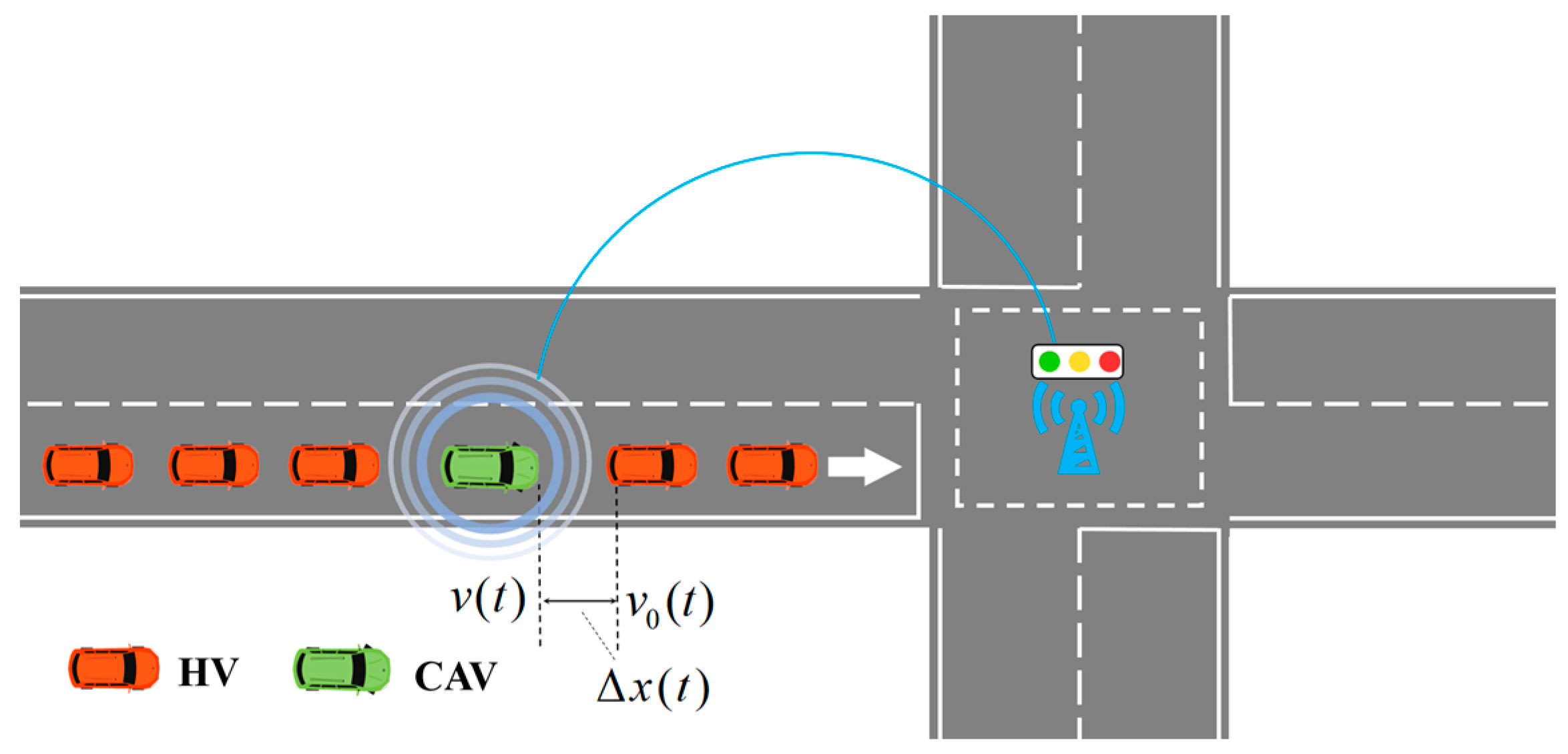
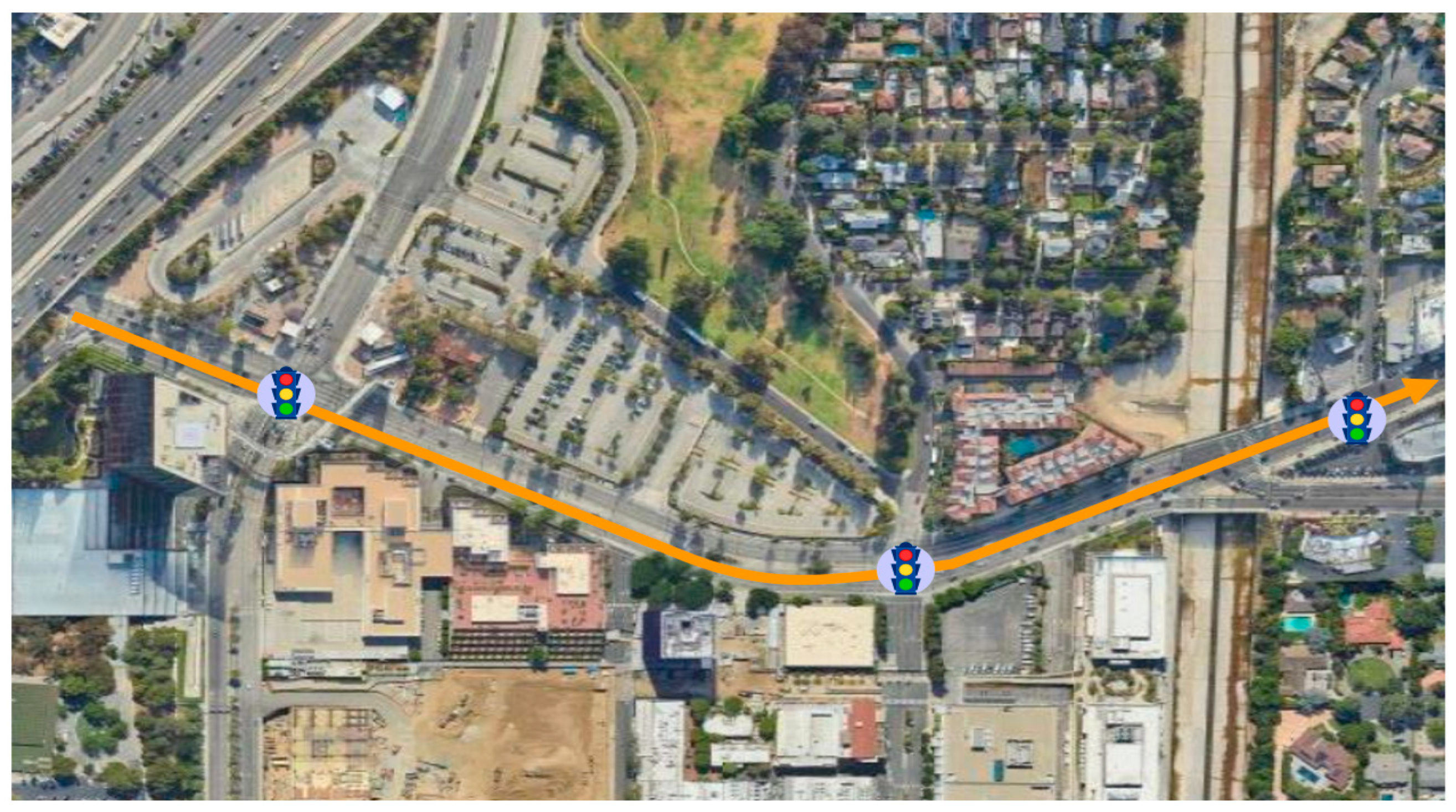
2.1. Research Scenario

This paper presents a research scenario where a CAV is integrated into a manually driven traffic flow to explore a single-vehicle control strategy. As depicted in Figure 1, all vehicles maintain their lanes without any lateral lane-changing. The traffic flow includes a mix of human-driven vehicles (HVs) and the CAV. The HVs adhere to a traditional driving model, while the CAV employs a specifically designed control algorithm for longitudinal following.

The traffic system enables data exchange through communication technologies at the intersection. Equipped with onboard sensors, the CAV interacts with nearby vehicles to gather real-time data on the speed and position of the vehicle ahead, adjusting its speed to maintain a safe distance. Moreover, the CAV accesses vital SPaT information by connecting with roadside units. These SPaT data allow the system to calculate the remaining green-light time, aiding the CAV in deciding whether to speed up or slow down.

2.2. Description of MDP

The strategy for navigating the CAV through signalized intersections is developed as a Markov decision process (MDP) [34]. This MDP framework for CAV control considers various factors, including the vehicle’s velocity and location, information from the preceding vehicle, and the current state of traffic signals. The framework operates under the following assumptions:

(1)

The road is solely used by motor vehicles in prime driving condition, adhering to established regulations and free from unforeseen incidents like malfunctions or erratic intrusions;

(2)

Real-time information regarding the vehicle’s position, speed, and acceleration is accessible. Simultaneously, real-time communication between onboard devices and roadside equipment is assured, without any delays.

2.2.1. State

The state in this context should encompass the dynamics of the CAV, the conditions of surrounding vehicles, and the status of traffic lights. Consequently, a multi-element vector is constructed to depict the CAV’s state:

$$S_t={[x_t,v_t,a_t,\Delta x_t,\Delta v_t,{\varphi }_t,g_t]}^T,$$

(1)

where $S_t$ denotes the state space at time $t$, $x_t$ is the travel distance of the vehicle, $v_t$ denotes the speed of the vehicle, $a_t$ denotes the acceleration of the vehicle, $\Delta v_t$ is the differential value of speed between the preceding and following vehicles, and $\Delta x_t$ is the spacing distance between the preceding and following vehicles.

Additionally, the signal lamp’s status is represented as ${\varphi }_t$ in (1), assigning a value of 1 for a red signal and 0 otherwise, and $g_t$ denotes the remaining duration of the green light in the current phase at the nearest signalized intersection. This definition of state remains relevant whether the vehicle is on a road segment or within an intersection. Consequently, the framework can naturally extend to accommodate a multi-intersection scenario.

2.2.2. Action

Upon acquiring pertinent information from the state space, the vehicle is required to respond dynamically based on acquired state information. This involves immediate adjustments in speed achieved through continuous acceleration and deceleration actions. Consequently, the action space ($A_t$) is identified by the acceleration of the vehicle, illustrated by (2).

$$A_t=a_t$$

(2)

Highlighting the importance of realism, acceleration ($a_t$) within the action space should comply with a specific interval ($d_{min}\le a_t\le a_{max}$, where $d_{min}$ and $a_{max}$ respectively represents the vehicle’s maximum allowable acceleration and deceleration, respectively, based on its specifications). Additionally, considering road traffic regulations and the safe operation of vehicles, it is essential to observe the following constraints:

$$v_{t-1}+a_t<v_{max}$$

(3)

$${\displaystyle {\int }_0^{\Delta t}(v_{t-1}+a_t)\Delta tdt<\Delta x^{*}}$$

(4)

where $v_{max}$ denotes the maximum speed limit of the road, and $\Delta x^{*}$ is the minimum safety distance between the front and rear vehicles.

By utilizing the state-space parameters as input for the environment and defining reward functions as objectives, we employ RL algorithms to train the agent. The aim is to obtain an optimal sequence of actions that maximizes rewards, thereby optimizing system performance. The optimal action sequence represents the CAV’s most efficient driving strategy.

2.2.3. Reward

When tackling the control challenges faced by CAVs at intersections, it is imperative to consider a range of factors, notably energy consumption and traffic efficiency among others. To comprehensively optimize the driving process of CAVs and attain optimal performance, this study designs a multi-objective reward function that considers diverse aspects to efficiently train agents. Specifically, the reward function aims to minimize energy consumption, mitigate traffic delays, and enhance driving comfort, all while prioritizing safety.

For the component of travel efficiency, the reward function utilizes the vehicle’s travel distance at each step as it crosses intersections, as detailed in Equation (5).

$$r_1=\left|x_t-x_{t-1}\right|$$

(5)

To reduce the electric energy consumption of the CAV at intersections, the reward function ($r_2$) for the energy consumption component is presented in (6).

$$r_2=(1-\eta )[E_{veh}(v_t,a_t,x_t)-E_{loss}(v_t,a_t,x_t)],$$

(6)

where $\eta$ denotes the energy recovery factor, $E_{veh}$ is a function capable of yielding the instantaneous electric energy of the CAV, and $E_{loss}$ represents the energy loss caused by the driving resistance. $E_{veh}$ and $E_{loss}$ incorporate principles from vehicle dynamics and energy conversion, respectively, considering the energy brake-recovery mechanism. Specific details can be referenced in [35].

Safety is always the top priority in vehicle operation. Here, the reward function ($r_3$) is formulated around time to collision (TTC), imposing greater penalties for actions that breach the safety margin, as demonstrated in (7).

$$r_3=\{\begin{array}{l}{e}^{\alpha \cdot TT{C}^{*}\cdot \left(\frac{\Delta v_t}{\Delta x_t}\right)},TT{C}_t<TT{C}^{*}\\ 0,otherwise\end{array},$$

(7)

where $\alpha$ is penalty coefficient for dangerous driving, $TT{C}_t$ denotes the time to the collision between the preceding and following vehicles at time $t$, and $TT{C}^{*}$ is the pre-defined safety threshold of $TT{C}_t$, selected as 2 s according to previous literature [36].

Enhancing driving comfort entails maintaining the smooth operation of the vehicle, reducing abrupt accelerations and decelerations to achieve a relatively smooth driving trajectory. Jerk, the derivative of acceleration, is used to characterize the stability of vehicle driving. The reward function ($r_4$) for driving comfort is calculated by (8) and (9).

$$r_4=\{\begin{array}{l}\beta \left(\left|J_t\right|-J^{*}\right),\left|J_t\right|>J^{*}\\ \\ 0,otherwise\end{array}$$

(8)

$$J_t=\frac{d{a}_t}{dt},$$

(9)

where $\beta$ is the penalty coefficient for aggressive driving, $J_t$ denotes the jerk of the vehicle at the time $t$, and $J^{*}$ represents the maximum permissible rate of change in acceleration that enables the vehicle to drive smoothly. According to previous research experience [37], the value of $J^{*}$ can be taken as 4.

Ultimately, the overall reward function ($R_t$) is derived by integrating the reward functions across all four indices, as shown in (10).

$$R_t=r_1-{\displaystyle \sum _{i=2}^4{r}_i}$$

(10)

3. Design and Analysis of Algorithm

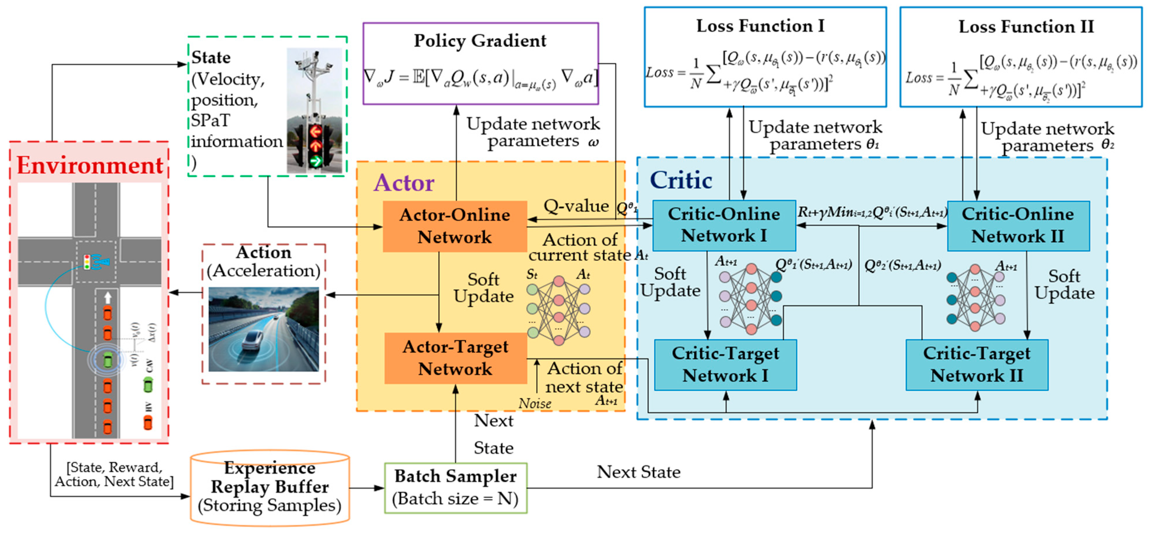
3.1. TD3 Algorithm

The TD3 algorithm is the chosen training method in the environmental framework. Within reinforcement learning, several classical training algorithms merit consideration, such as the Deep Q-Network (DQN) algorithm and the Deep Deterministic Policy Gradient (DDPG) algorithm. The DQN algorithm relies on a learned value function, known as the Q-function, and integrates crucial techniques such as sample pooling and target networks [38,39]. However, DQN is primarily effective for tasks with a limited range of discrete actions and faces limitations in scenarios requiring real-time decisions, such as car-following on roads. To effectively address the reinforcement learning problem with continuous actions, the DDPG algorithm is introduced [40]. DDPG merges the value function and the policy gradient algorithm, improving parameter updates and facilitating seamless decision-making in continuous action spaces.

Nonetheless, certain algorithm-level issues persist in DDPG, such as overestimation bias and susceptibility to overfitting of narrow peaks in the value estimate. As a remedy, TD3 (Twin Delayed DDPG) is introduced to address these shortcomings in the DDPG algorithm [41]. Compared with DDPG algorithm, the TD3 algorithm uses a double critic network to calculate the target value of Q-functions, opting for the lesser of the two values, thus suppressing the problem of network overestimation.

As illustrated in Figure 2, the network structure of the TD3 algorithm is composed of the actor policy network and a critical value network. The actor network is responsible for determining optimal actions, while the critic network evaluates the desirability of these actions by estimating values of Q-functions. To enhance training stability, the target network periodically updates its parameters by copying them from the current network. Additionally, the delayed policy update is employed to ensure that the actor network is updated after the critic network undergoes multiple updates.

TD3 employs a parameterized actor neural network, which takes the state ($S_t$) as input and generates a continuous action ($A_t$) as output. Simultaneously, a parameterized critic neural network is utilized to take both the state ($S_t$) and action ($A_t$) as inputs and estimate the Q-value function. The parameters of the algorithm are manually adjusted through extensive simulations. Both the actor and critic neural networks utilize a two-hidden-layer architecture employing a multi-layer perceptron (MLP). The first layer of both the actor and critic networks consists of 400 neurons, while the second layer comprises 300 neurons.

The network structure of the TD3 algorithm is intricately designed with distinct roles for each component. The actor network serves as the interface with the external intersection environment, managing the input and output of data. Concurrently, the set of transitions $\left(S_t,A_t,R_t,S_{t+1}\right)$ is systematically added to the experience replay pool as samples for future training iterations. Action parameters ($A_t$) are transferred from the actor network to the critic network. The double critic networks are employed, selecting the minimum value between $Q^{{\theta }_1\prime }\left(S_{t+1},A_{t+1}\right)$ and $Q^{{\theta }_2\prime }\left(S_{t+1},A_{t+1}\right)$ when calculating the target value, to mitigate the issue of network overestimation in the algorithm. For a set of data from the sample pool, the dual critic-target network calculates the target value ($y$) according to (11).

$$y=R_t+\gamma \underset{i=1,2}{min}{Q}^{{\theta }_i\prime }\left(S_{t+1},A_{t+1}\right),$$

(11)

where $\gamma$ is the discount factor for reward $R_{t+1}$, ${\theta }_i\prime$ denotes the parameter of critic-target networks I and II, and $Q^{{\theta }_i\prime }\left(S_{t+1},A_{t+1}\right)$ represents the estimated Q-value according to the state and action.

Target policy smoothing is implemented in TD3 as a regularization technique. Its purpose is to constrain the action values by clipping them according to the target policy, ensuring that the actions remain within a valid action range ($A_t\in \left[A_{low},A_{high}\right]$). Then, the target action can be expressed as follows:

$$A_{t+1}=clip\left({\mu }_{{\theta }_i\prime }(S_{t+1})+ϵ,A_{low},A_{high}\right),$$

(12)

where ${\mu }_{{\theta }_i\prime }(S_{t+1})$ denotes the action strategy adopted in state $S_{t+1}$, and $ϵ\sim (0,\sigma )$ is random Gaussian noise. Subsequently, the target value ($y$) is transmitted to dual critic-online networks I and Ⅱ. Here, the current Q-value is recalculated, and the network parameters are updated to minimize the loss function ($L$) as follows:

$$L_{{\theta }_i}=\frac{1}{N}{\displaystyle \sum _{i=1}^2{\left[Q^{{\theta }_i}(S_t,{\mu }_{{\theta }_i}(S_t)+ϵ)-y\right]}^2}$$

(13)

where $N$ denotes the batch size, ${\theta }_i$ is the parameter of critic-online networks I and Ⅱ, and $Q^{{\theta }_i}(S_t,{\mu }_{{\theta }_i}(S_t)+ϵ)$ represents the target Q-value. Through this optimization, parameter ${\theta }_i$ of the critic is adjusted to enhance the accuracy of Q-value predictions. Parameter ${\theta }_i\prime$ of the target network is updated smoothly from the main network as follows:

$${\theta }_i\prime =\tau {\theta }_i\prime +\left(1-\tau \right){\theta }_i,$$

(14)

where $\tau$ is a hyperparameter to determine the weight. Subsequently, the Q-value ($Q^{{\theta }_1}(S_t,{\mu }_{\omega }(S_t))$) calculated by critic network I is transmitted to the actor network to update parameters. Then, the actor can be updated by the deterministic policy gradient (${\nabla }_{\omega }J$) as follows:

$${\nabla }_{\omega }J=\mathbb{E}\left[{\nabla }_a{Q}^{{\theta }_1}(S_t,a){|}_{a={\mu }_{\omega }(S_t)}{\nabla }_{\omega }a\right],$$

(15)

where $\omega$ denotes the parameter of the actor network.

3.2. Vehicle Control Algorithm

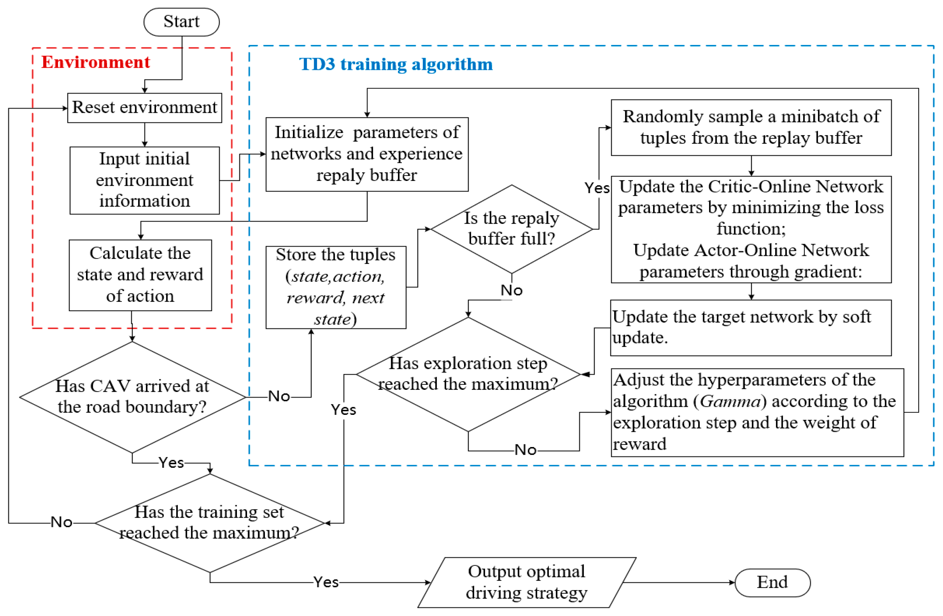
The control algorithm for CAVs is developed within the MDP environment framework, leveraging the network architecture of the TD3 training algorithm. This algorithm takes the speed, position, signal phase, and timing information obtained from vehicle sensors as input. Through the training process, the algorithm outputs an action strategy to the vehicle controller for optimization of acceleration, ensuring smoother, safer, and more efficient driving behaviors.

Additionally, as the vehicle approaches intersections, the algorithm undertakes a detailed assessment of traffic signals. Specifically, it evaluates whether the remaining duration of the green light is sufficient for the vehicle to navigate the intersection smoothly and safely. Following this analysis, the algorithm issues precise commands to the vehicle controller, directing it to accelerate or decelerate as necessary. The flow chart of this algorithm is shown in Figure 3.

The environmental input data involve collecting information on the vehicle’s speed ($v_t$), position ($x_t$), and signal light status, including the current status of signal lamps (${\varphi }_t$) and the remaining duration of the green light ($g_t$). Through multiple iterations equal to the number of training epochs multiplied by the ratio of sample volume to batch size, the action strategy with the maximum reward, namely the optimal acceleration, is output to control the vehicle. The algorithm proceeds through the following specific steps:

Step1.

Initialization: Upon initiation, the environment state ($S_t$) is reset, and essential road and traffic demand data are transmitted to the vehicle controller. The TD3 algorithm receives state information, including speed, position, and SPaT. It initializes action ($A_t$) and provides a predicted sequence of actions to the environment.

Step2.

Interaction with the environment: After receiving the action sequence, the environment calculates the reward ($R_t$) of the vehicle until it approaches the road boundary. Subsequently, the calculated state and reward are transmitted back to the controller. The TD3 algorithm stores these tuples $\left(S_t,A_t,R_t,S_{t+1}\right)$ in the experience pool, accumulating valuable training samples.

Step3.

Training: Training begins once the replay buffer reaches its capacity, utilizing the stored samples to refine decision-making for vehicle actions. The algorithm continues training until the maximum exploration step is reached, signifying the conclusion of the current episode of training. Upon reaching the maximum number of iterations, the algorithm indicates the attainment of the terminal state.

Step4.

Output: The algorithm outputs a control strategy ($\pi \left(a_t\right)$) for driving actions, including uniform speed, acceleration, and deceleration. This strategy is meticulously designed to maximize cumulative rewards ($R^{*}$), reflecting the algorithm’s learned optimal behavior in response to the dynamic road environment and traffic conditions.

4. Examples and Discussion

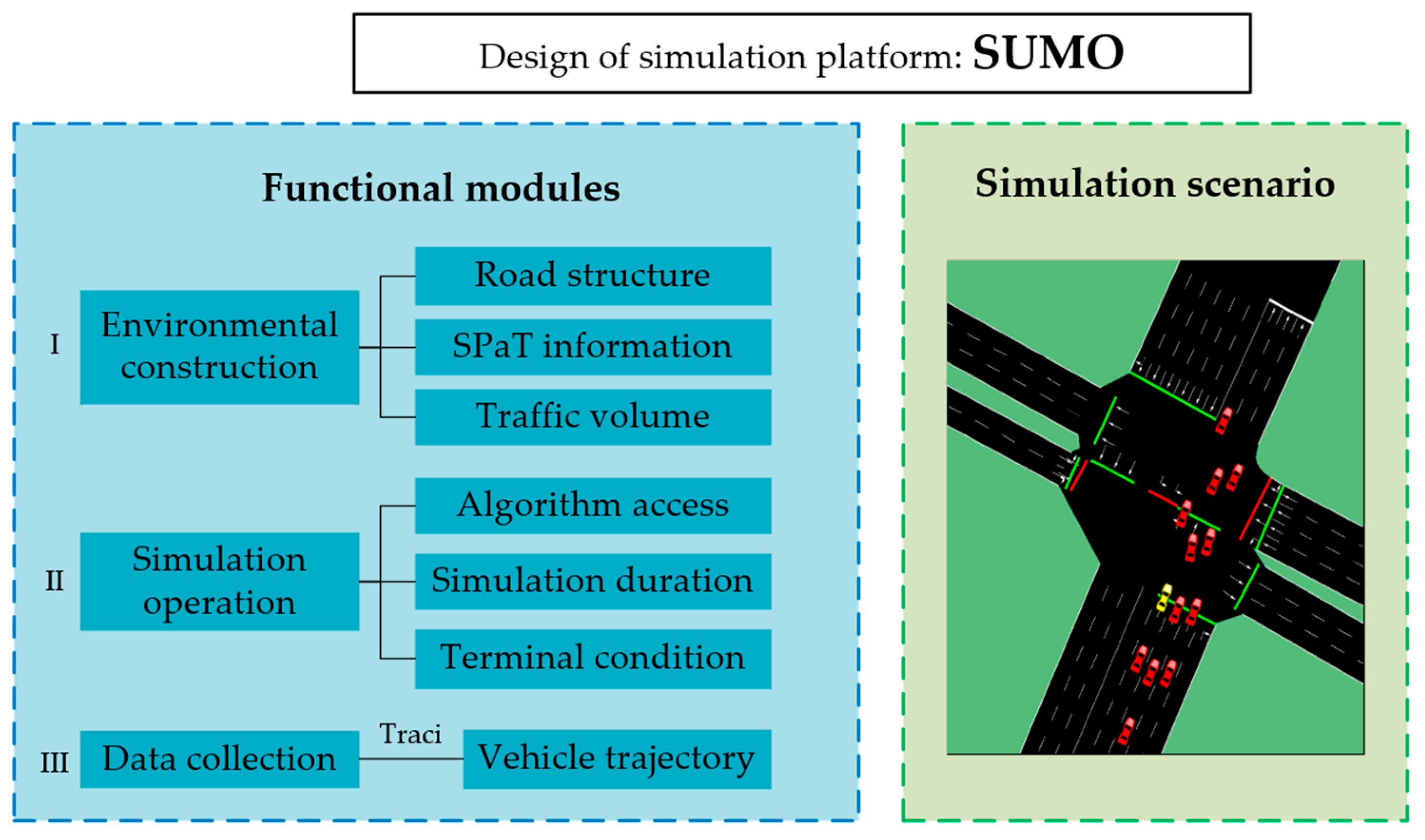
4.1. Simulation Platform and Scenarios

To validate the proposed control method for CAVs, this study utilizes SUMO simulation software to develop an intersection traffic simulation platform. The simulation platform integrates various components seamlessly, ensuring a comprehensive evaluation of the proposed control method for CAVs. This platform adopts a modular simulation approach, featuring a visual interface, result data collection, and other essential functions. The detailed architecture of this simulation platform is illustrated in Figure 4, providing a visual representation of the component interactions and their contributions to the system’s overall functionality. The functional modules of the simulation platform illustrated in Figure 4 are described in detail in

Table 1. Functional modules of simulation platform.

Functional Module	Description
Environmental construction	This module is responsible for creating and editing the road network, with specific functions such as determining the starting and ending points, adding traffic demands, dividing the lanes, and configuring signal timing.
Simulation operation	This module is responsible for running the simulation program, with specific functions including setting the simulation duration, calculating the state space and reward function, and outputting the action strategy, as well as resetting the environment when the algorithm training termination conditions are met.
Data collection	This module is responsible for data acquisition and saving, with specific functions including acquiring vehicle trajectory data through the Traci interface, saving the simulation results in a numerical matrix, and outputting the data in *.csv file format for later organization and analysis.

.

Within the platform, SUMO constructs the fundamental simulation environment and supplies the RL framework with essential simulation outcome data. Through the Traci interface, the RL framework retrieves critical information for the evaluation, including intersection geometry information (lane and signal IDs), vehicle dynamics (speed, acceleration, and driving distance), and signal timing details (signal phase duration). Subsequently, an interactive environment integrating multiple data sources is developed to evaluate vehicle control algorithms via the RL framework.

For the analysis and verification of the proposed control method’s effectiveness, this study establishes a simulation scenario utilizing road map information and signal timing data from Lankershim Boulevard, featured in the Next Generation Simulation (NGSIM) dataset. Several experiments are carried out in this simulation scenario to assess the performance of the CAV, providing a comprehensive examination of the control method’s real-road applicability.

Figure 5 illustrates a simulation scene with four adjacent urban signalized intersections along Lankershim Boulevard. Upon entering each intersection, vehicles receive pertinent environmental information. The mixed traffic flow on the road is composed of the CAV and HVs, with HVs following SUMO’s default Krauss car-following model and the CAV being algorithmically controlled. This research focuses on investigating the longitudinal car-following behavior of the CAV within mixed traffic flow, with known parameters such as signal timing and road length. In the experiment, the Krauss model and three RL algorithms, namely TD3, DDPG, and DQN, are adopted to govern the car-following movement of the CAV. Data from the simulation are gathered across various car-following modes for subsequent comparison and analysis.

4.2. Experimental Design and Parameters Settings

The simulation experiment’s core modules in the RL environment consist of road network setup, agent state space and reward function calculation, simulation execution, and environmental resetting following each run. Road network setup involves determining start and end points and lane segmentation and linking, along with configuring signal timings. Information on simulated vehicles and roads is sourced from Traci for state-space computation. The overall reward in this simulation experiment is calculated by evaluating crucial factors, including energy consumption per unit, travel distance, estimated collision time, and driving comfort. Moreover, the environmental reset process entails clearing all data before each training episode to initialize the simulation environment. In the simulation operation module, the vehicle is programmed to terminate the simulation once it has traversed beyond the entire road length and subsequently returns state and reward values to the main function after each iteration. Data from the simulations are stored in a numerical matrix format and outputted as text files for ease of sorting and analysis.

Four distinct control methods, namely the Krauss model, TD3, DQN, and DDPG, are employed for longitudinal following of the CAV during intersection navigation. Additionally, the lateral lane-changing behavior of vehicles is governed by the SUMO default lane-changing model (LC2013) [42]. Experiments are conducted to assess and compare the performance of the CAV under each control method to identify the most effective one. To alleviate the impact of the preceding vehicle on the training vehicle and prioritize safety, default values for speed differential and relative distance in state space are set as maximum speed limits and safety thresholds. For structural parameters, current market performance parameters for electric vehicles are used, and drag coefficients for vehicle motion are sourced from existing studies [43]. In addition, the hyperparameter of the RL algorithm is determined through numerous experiments. A hyperparameter in machine learning refers to a configuration setting that influences the behavior and performance of a model during training, yet it cannot be directly learned from the data. Examples include learning rate, batch size, and discount factor. It is imperative to maintain consistency in environmental parameters across simulations, encompassing road and vehicle attributes. These essential parameters for simulation fidelity are detailed in

Table 2. Simulation parameter settings.

Parameter	Value
Design hour volume of HVs (veh/h)	1600
Total driving distance (m)	525
The speed limit (km/h)	40
Vehicle acceleration (m/s2)	(−4.500, 4.500)
Minimum safety distance between front and rear vehicles (m)	30
Green time (s)	[41, 37, 64, 46]
Yellow time (s)	[3.50, 3.90, 3.50, 3.50]
All-red time (s)	[0.50, 1.50, 1.00, 1.00]
Maximum training steps	105
Batch size	256
Learning rate	10−4
Discount factor	0.98

.

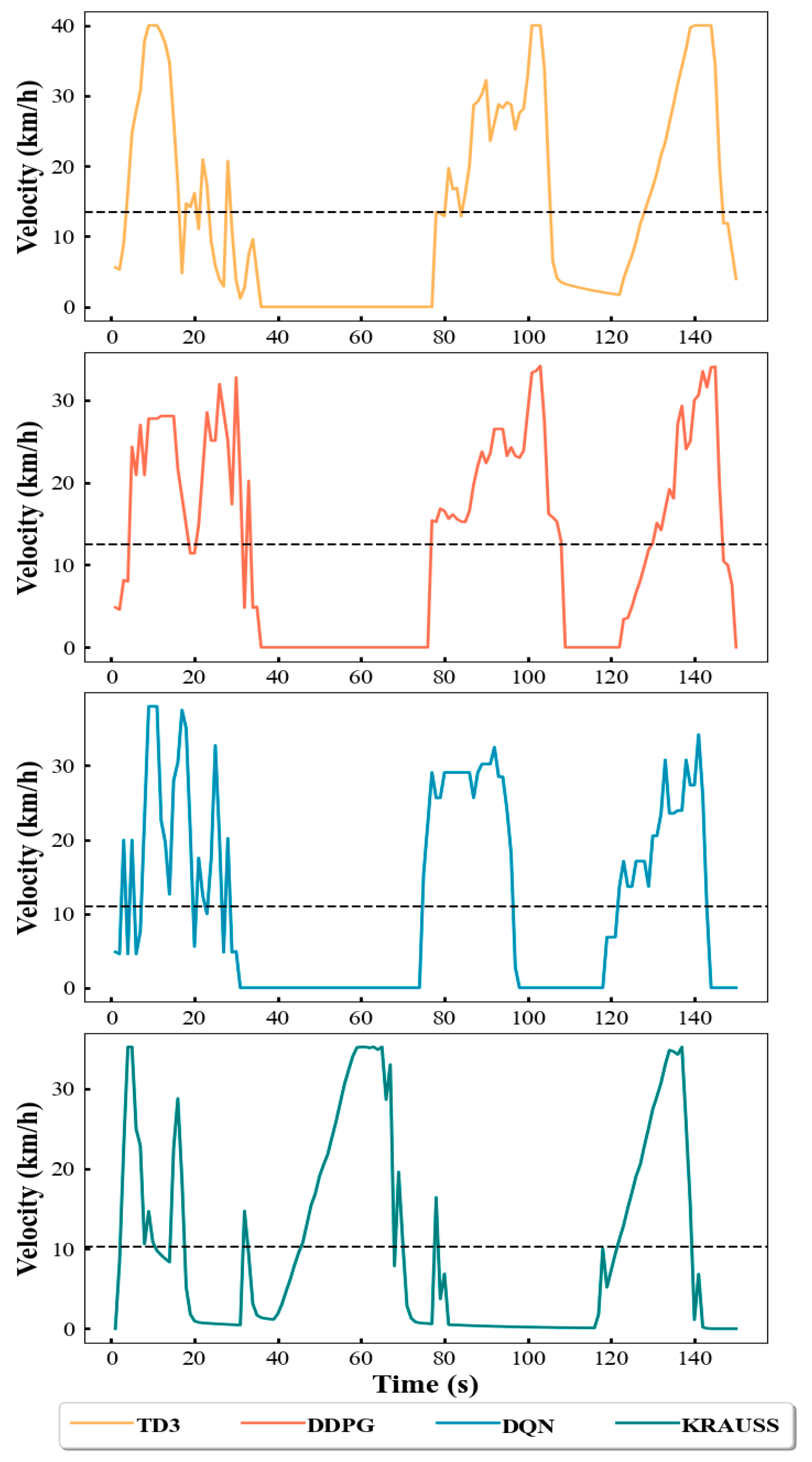
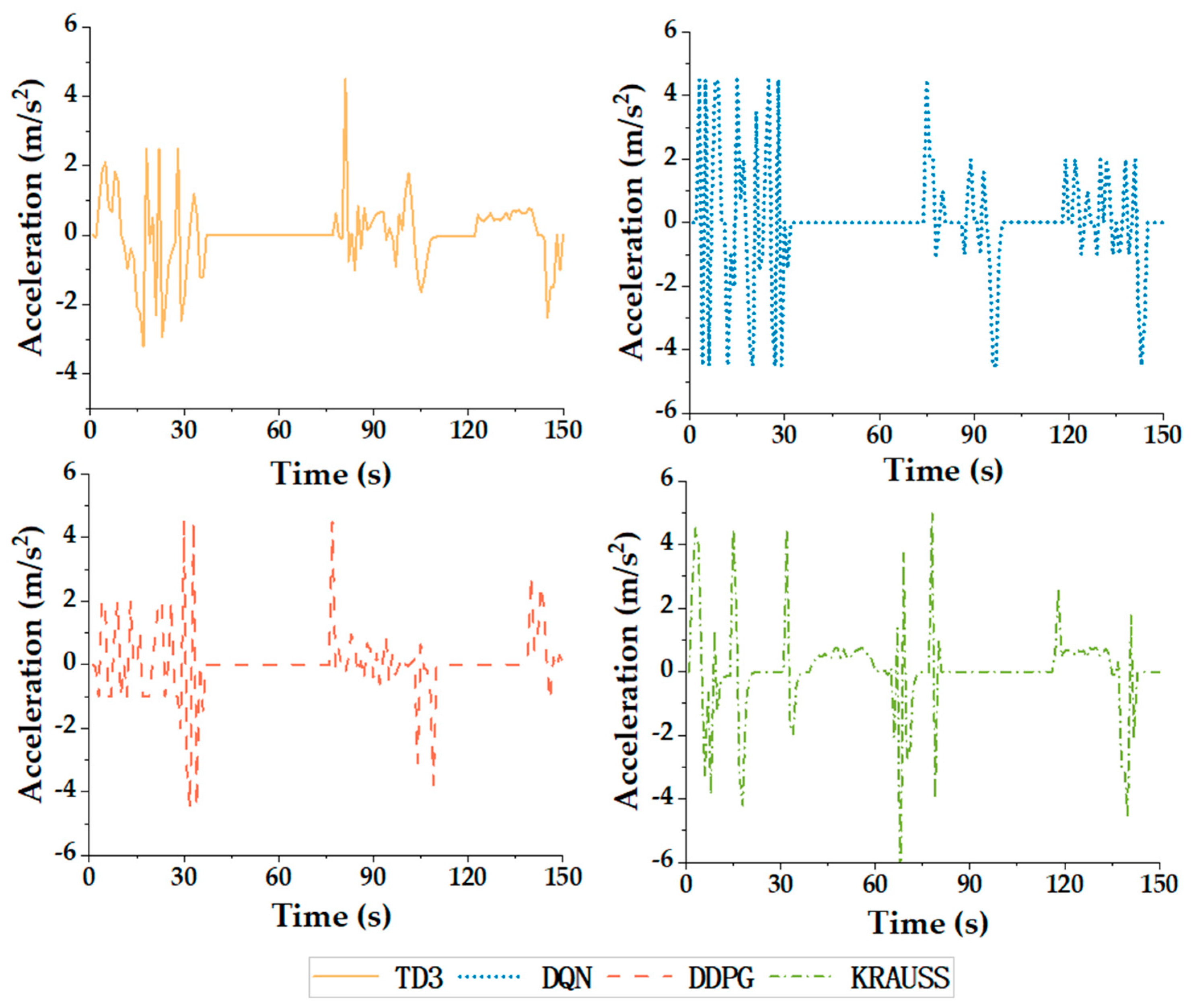
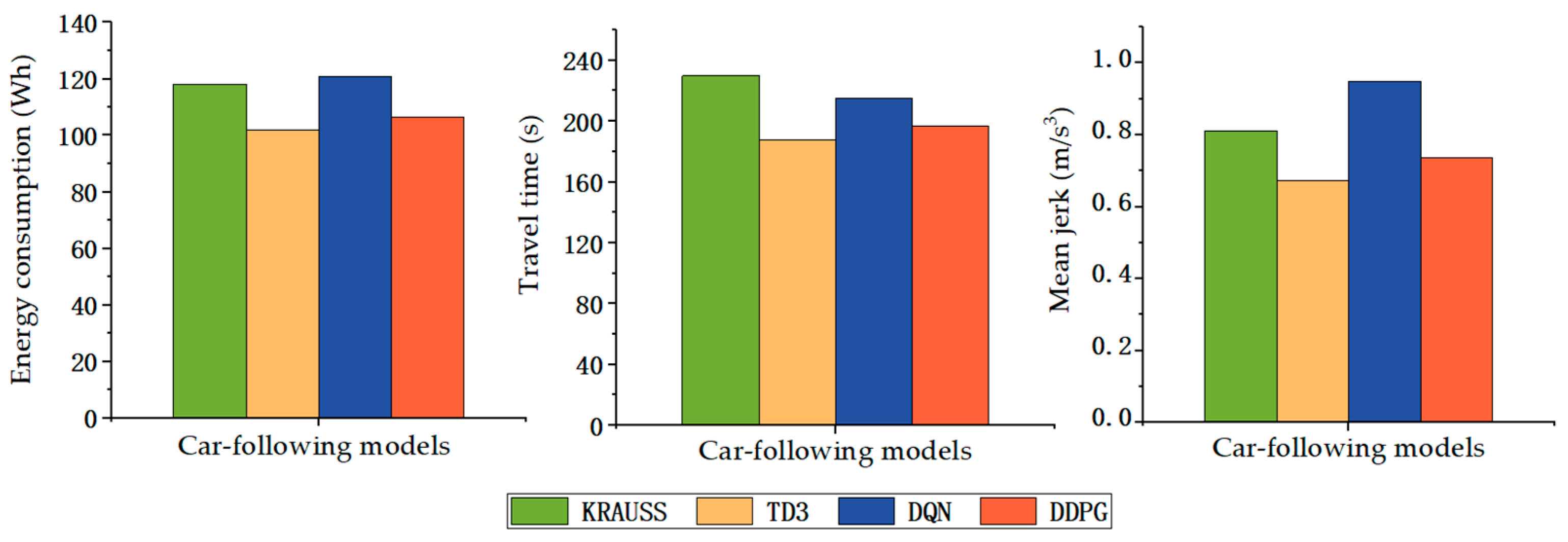
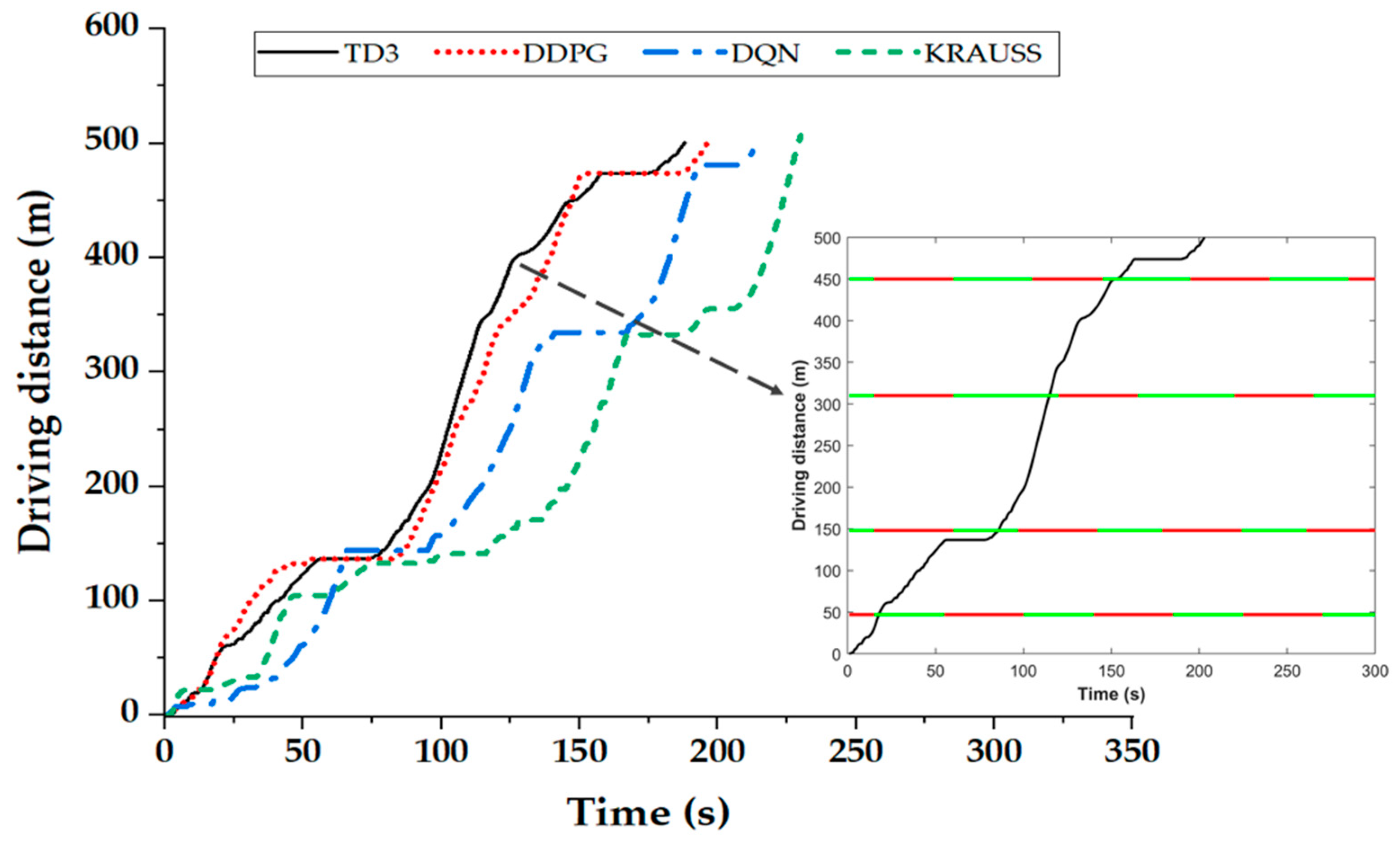
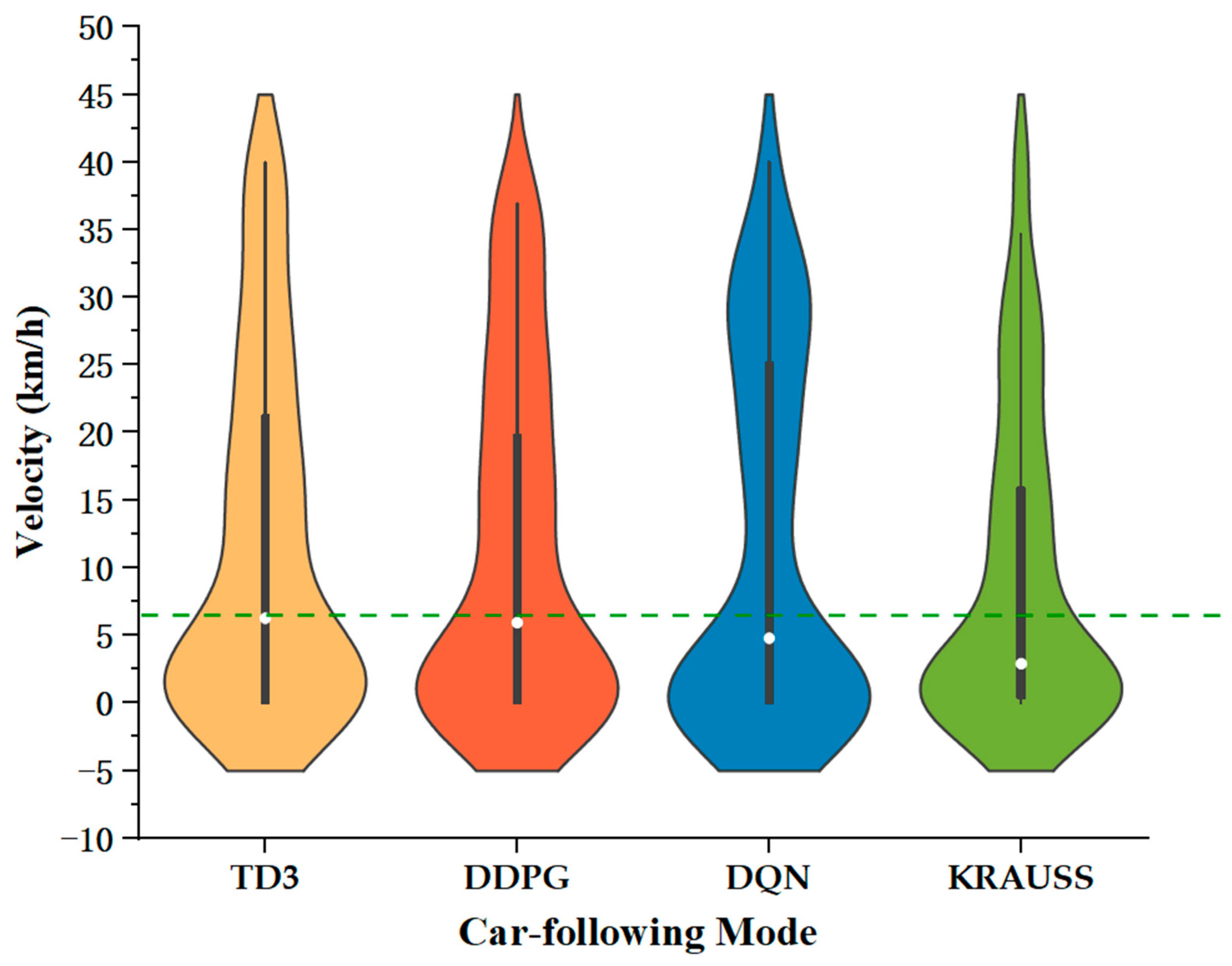
4.3. Simulation Results and Discussion

Data from the simulation experiments are meticulously processed to analyze the vehicle’s motion characteristics under Krauss, TD3, DDPG, and DQN car-following modes. Regarding the safety aspect of CAV driving, it is noteworthy that unsafe driving behavior is initially observed in the early iterations of the algorithm simulation, where the time to collision exceeds the predefined safety threshold. However, such instances cease to occur in subsequent iterations. This is attributed to the penalty mechanism implemented in the reward function, where a significant penalty is assigned to driving behaviors violating safety protocols, while actions complying with safe driving norms receive equal reward values. Essentially, safety rewards are structured to enforce safe driving as a non-negotiable prerequisite.

In summary, given that across all modes, the CAV adheres to the fundamental requirement of safe driving, as evidenced by consistent safety reward values, our comparative analysis focuses on energy consumption, efficiency, and driving comfort among the different approaches. Notably, “efficiency” refers to the effectiveness of a vehicle’s movement, quantified by factors such as travel time and mean velocity across intersections. The specific evaluation indicators include electricity consumption, travel time, and mean jerk. Findings are summarized in

Table 3. Simulation results under different car-following modes.

Car-Following Mode	Evaluation Indicators
	Electricity Consumption (Wh)	Travel Time (s)	Mean Jerk (m/s3)
TD3	101.845	188	0.674
DDPG	106.463	197	0.736
DQN	120.943	215	0.949
KRAUSS	118.102	230	0.811

.

The vehicle’s motion performance, analyzed using various indices, is depicted in Figure 6. Regarding efficiency and comfort, the TD3 algorithm exhibits superior performance over the other three car-following modes. For energy consumption, this study delves into the electric energy consumed by the CAV to evaluate vehicle performance across various car-following modes. The application of the TD3 algorithm in CAV training significantly reduces driving energy consumption—4.33%, 15.79%, and 13.77% compared to DDPG, DQN, and Krauss, respectively. This underscores the proposed algorithm’s outstanding effectiveness in energy conservation.

Based on trajectory data from simulations, a vehicle spacetime diagram is generated for intuitive comparison and analysis of vehicle traffic efficiency under various car-following modes. As illustrated in Figure 7, the CAV trained by the TD3 algorithm exhibits the longest driving distance per unit of time during most periods. Since the TD3 algorithm is an improvement on the DDPG algorithm, the curves corresponding to these two algorithms are very close in Figure 7. However, the action strategy obtained under DDPG algorithm training has an increased magnitude of variation at the beginning, as evidenced by the vehicle starting with greater acceleration. Although the CAV trained by DDPG reaches the first intersection in a shorter time during the initial phase of the vehicle’s travel, it consumes more waiting time at the same time.

On the other hand, the CAV controlled by the TD3 algorithm travels at a relatively continuous speed overall and spends less time at intersections. Therefore, in terms of the final results, the TD3-controlled CAV consumes the shortest amount of travel time to travel the entire length of the road. The TD3 mode incurs time cost reductions of 4.57%, 12.56%, and 18.26% compared to DDPG, DQN, and Krauss, respectively. This emphasizes the effectiveness of the TD3 algorithm in enhancing travel time efficiency.

As the CAV controlled by the TD3 algorithm approaches each intersection, it receives SPaT information from roadside equipment, which is then used to determine the remaining duration of the green light in the current phase. Employing this algorithm enables the determination of whether a smooth intersection passage can be achieved, subsequently allowing for judicious acceleration or deceleration actions. Therefore, optimal algorithmic control effectively reduces the time spent by the CAV to stop and wait at red lights while maintaining a high average velocity.

Figure 8 illustrates a violin diagram depicting the velocity distribution, offering a detailed analysis of the speed characteristics of the CAV. With TD3 algorithm training, the speeds of the CAV are notably concentrated in a higher range, achieving the highest average speed in comparison to other car-following modes.

Figure 9 compares the characteristics of the CAV‘s speed changes in various car-following modes. As depicted, the vehicle requires prompt speed adjustments near intersections, resulting in noticeable upward or downward shifts in the curve. Moreover, under the intelligent control of RL algorithms, the velocity of the CAV significantly improves compared to the traditional car-following model, with the TD3 algorithm reaching a relatively higher peak. The data reveal that the average driving speeds attained by TD3, DDPG, DQN, and Krauss modes are 13.41 km/h, 12.48 km/h, 11.01 km/h, and 10.46 km/h, respectively. In comparison with the DQN, DDPG, and Krauss modes, the TD3 mode demonstrates significant increases in average driving speed of 7.45%, 21.80%, and 28.20%, respectively. This underscores the effectiveness of the proposed method in enhancing the speed performance of the CAV.

The jerk during vehicle operation is utilized as an index for evaluating driving comfort, reflecting sudden speed changes as the CAV navigates through intersections, thereby indicating the smoothness of vehicle operation. Figure 9 visually represents the variation in acceleration during CAV driving under different car-following modes. As depicted in Figure 10, both the DQN and DDPG modes show considerable fluctuations in driving behavior, whereas the TD3 mode maintains more stable acceleration, mostly within the range of [−3, 4]. Comparative analysis of four car-following modes reveals that in the TD3 car-following mode, the CAV acceleration curve is notably flat, and the average jerk is the smallest. This behavior is attributed to its driving pattern, which is characterized by gradual acceleration or early deceleration. Compared with the DDPG, DQN, and Krauss modes, the jerk is reduced by 8.42%, 28.97%, and 16.89%, respectively. This suggests that the CAV trained with TD3 shows notably better stability in driving performance.

5. Conclusions

An RL-based control method is proposed for CAVs at signalized intersections, aiming to optimize vehicle performance by holistically addressing energy consumption, traffic efficiency, driving comfort, and safety. The MDP framework for CAV driving is specifically tailored for multi-intersection environments, with the driving strategy trained by the TD3 algorithm. Furthermore, simulations of urban scenarios with multiple intersections are conducted to investigate the motion characteristics of the vehicle under various car-following modes. Results indicate that the proposed methods yield a 13.77% reduction in energy consumption and a notable 18.26% decrease in travel time. The findings reveal that this method allows the CAV to dynamically adjust to traffic conditions, improving travel efficiency and driving comfort, which can also lead to reduced fuel consumption.

Since the simulation experiment reported in this paper is conducted under ideal conditions, within a scene devoid of random occurrences such as spontaneous overtaking or abrupt failures, the simulation is a valid testbed for the testing of algorithmic behavior. Notably, changes in factors such as traffic density, communication network reliability, and vehicle characteristics can lead to variations in simulation results. In practical use, considering the lack of perfect cooperation between CAVs and existing transportation infrastructure and the delay of communication systems, the actual optimization effect may require percentage correction, which will be scrutinized in a subsequent study.

The primary research focus of this paper is to utilize RL algorithms to control a single agent, specifically addressing the longitudinal car-following behavior of an individual CAV. Due to the potential for the variance of the gradient to escalate with an increasing number of agents, it becomes imperative to devise and implement multi-agent RL algorithms. Moreover, reducing the dimensionality of the state space becomes essential, particularly for traffic scenarios featuring multiple CAVs. This represents one of the key research directions we aim to advance in the future. Future research will also focus on the lateral motion of CAVs on the road, combining lane-changing models to thoroughly study the driving behavior of vehicles. Moreover, a comprehensive analysis will be conducted from the perspective of traffic flow to discuss the method under different CAV permeabilities, affording deeper insight into the proposed control strategy.

References

1. De Campos, G.R.; Falcone, P.; Hult, R.; Wymeersch, H.; Sjöberg, J. Traffic coordination at road intersections: Autonomous decision-making algorithms using model-based heuristics. IEEE Intell. Transp. Syst. Mag. 2017, 9, 8–21. [Google Scholar] [CrossRef]
2. Li, Y.; Chen, B.; Zhao, H.; Peeta, S.; Hu, S.; Wang, Y.; Zheng, Z.D. A car-following model for connected and automated vehicles with heterogeneous time delays under fixed and switching communication topologies. IEEE Trans. Intell. Transp. Syst. 2022, 23, 14846–14858. [Google Scholar] [CrossRef]
3. Deng, Z.; Shi, Y.; Han, Q.; Lv, L.; Shen, W.M. A conflict duration graph-based coordination method for connected and automated vehicles at signal-free intersections. Appl. Sci. 2020, 10, 6223. [Google Scholar] [CrossRef]
4. Zhang, J.; Cheng, Y.; He, S.; Ran, B. Improving method of real-time offset tuning for arterial signal coordination using probe trajectory data. Adv. Mech. Eng. 2017, 9, 1687814016683355. [Google Scholar] [CrossRef]
5. Saboohi, Y.; Farzaneh, H. Model for developing an eco-driving strategy of a passenger vehicle based on the least fuel consumption. Appl. Energy 2008, 86, 1925–1932. [Google Scholar] [CrossRef]
6. Shao, Y.; Sun, Z. Eco-approach with traffic prediction and experimental validation for connected and autonomous vehicle. IEEE Trans. Intell. Transp. Syst. 2021, 22, 1562–1572. [Google Scholar] [CrossRef]
7. Yu, C.; Feng, Y.; Liu, H.; Ma, W.; Yang, X. Integrated Optimization of Traffic Signals and Vehicle Trajectories at Isolated Urban Intersections. Transp. Res. B-Meth. 2018, 112, 89–112. [Google Scholar] [CrossRef]
8. Jiang, H.; Jia, H.; Shi, A.; Meng, W.; Byungkyu, B. Eco Approaching at an Isolated Signalized Intersection under Partially Connected and Automated Vehicles Environment. Transp. Res. C-Emerg. Technol. 2017, 79, 290–307. [Google Scholar] [CrossRef]
9. Yang, J.; Zhao, D.; Jiang, J.; Lan, J.; Mason, B.; Tian, D.; Li, L. A less-disturbed ecological driving strategy for connected and automated vehicles. IEEE Trans. Intell. Veh. 2023, 8, 413–424. [Google Scholar] [CrossRef]
10. Kargar, M.; Zhang, C.; Song, X. Integrated optimization of power management and vehicle motion control for autonomous hybrid electric vehicles. IEEE Trans. Veh. Technol. 2023, 72, 11147–11155. [Google Scholar] [CrossRef]
11. Wu, X.; He, X.; Yu, G. Energy-optimal speed control for electric vehicles on signalized arterials. IEEE Trans. Intell. Transp. Syst. 2015, 16, 2786–2796. [Google Scholar] [CrossRef]
12. Li, M.; Wu, X.; He, X.; Yu, G.; Wang, Y. An eco-driving system for electric vehicles with signal control under v2x environment. Transp. Res. C-Emerg. Technol. 2018, 93, 335–350. [Google Scholar] [CrossRef]
13. Lu, C.; Dong, J.; Hu, L. Energy-efficient adaptive cruise control for electric connected and autonomous vehicles. IEEE Intell. Transp. Syst. Mag. 2019, 11, 42–55. [Google Scholar] [CrossRef]
14. Xia, H.; Boriboonsomsin, K.; Barth, M. Dynamic eco-driving for signalized arterial corridors and its indirect network-wide energy/emissions benefits. J. Intell. Transp. Syst. 2013, 17, 31–41. [Google Scholar] [CrossRef]
15. Lan, Y.; Han, M.; Fang, S.; Wu, G.; Sheng, H.; Wei, H.; Zhao, X. Differentiated speed planning for connected and automated electric vehicles at signalized intersections considering dynamic wireless power transfer. J. Adv. Transp. 2022, 2022, 5879568. [Google Scholar]
16. Du, Y.; Shang, G.; Chai, L.; Chen, J. Eco-driving method for signalized intersection based on departure time prediction. China J. Highw. Transp. 2022, 35, 277–288. [Google Scholar]
17. Li, Y.; Zhao, H.; Zhang, L.; Zhang, C. An extended car-following model incorporating the effects of lateral gap and gradient. Physica A 2018, 503, 177–189. [Google Scholar] [CrossRef]
18. Lv, Y.; Duan, Y.; Kang, W.; Li, Z.; Wang, F. Traffic flow prediction with big data: A deep learning approach. IEEE Trans. Intell. Transp. Syst. 2015, 16, 865–873. [Google Scholar] [CrossRef]
19. Jiang, X.; Zhang, J.; Wang, B. Energy-efficient driving for adaptive traffic signal control environment via explainable reinforcement learning. Appl. Sci. 2022, 12, 5380. [Google Scholar] [CrossRef]
20. Liu, C.; Sheng, Z.; Chen, S.; Shi, H.; Ran, B. Longitudinal control of connected and automated vehicles among signalized intersections in mixed traffic flow with deep reinforcement learning approach. Phys. A 2023, 629, 129189. [Google Scholar] [CrossRef]
21. Mousa, S.R.; Ishak, S.; Mousa, R.M.; Codjoe, J. Developing an eco-driving application for semi-actuated signalized intersections and modeling the market penetration rates of eco-driving. Transp. Res. Record 2019, 2673, 466–477. [Google Scholar] [CrossRef]
22. Jiang, X.; Zhang, J.; Li, D. Eco-driving at signalized intersections: A parameterized reinforcement learning approach. Transp. B 2022, 11, 1406–1431. [Google Scholar] [CrossRef]
23. Bin Al Islam, S.M.A.; Abdul Aziz, H.M.; Wang, H.; Young, S.E. Minimizing energy consumption from connected signalized intersections by reinforcement learning. In Proceedings of the 21st International Conference on Intelligent Transportation Systems (ITSC), Maui, HI, USA, 7 December 2018. [Google Scholar]
24. Guo, Q.; Ohay, A.; Liu, Z.; Ban, X. Hybrid Deep Reinforcement Learning based Eco-Driving for Low-Level Connected and Automated Vehicles along Signalized Corridors. Transp. Res. C-Emerg. Technol. 2021, 124, 2–18. [Google Scholar]
25. Qu, X.; Yu, Y.; Zhou, M.; Lin, C.; Wang, X. Jointly dampening traffic oscillations and improving energy consumption with electric, connected and automated vehicles: A reinforcement learning based approach. Appl. Energy 2020, 257, 114030. [Google Scholar] [CrossRef]
26. Chen, Y.; Jiao, P.; Bai, R.; Li, R. Modeling car following behavior of autonomous driving vehicles based on deep reinforcement learning. J. Transp. Inf. Saf. 2023, 41, 67–75. [Google Scholar]
27. Zhang, J.; Jiang, X.; Liu, Z.; Zheng, L.; Ran, B. A study on autonomous intersection management: Planning-based strategy improved by convolutional neural network. KSCE J. Civ. Eng. 2021, 25, 3995–4004. [Google Scholar] [CrossRef]
28. Tran, Q.-D.; Bae, S.-H. An Efficiency Enhancing Methodology for Multiple Autonomous Vehicles in an Urban Network Adopting Deep Reinforcement Learning. Appl. Sci. 2021, 11, 1514. [Google Scholar] [CrossRef]
29. Li, J.; Wu, X.; Fan, J. Speed planning for connected and automated vehicles in urban scenarios using deep reinforcement learning. In Proceedings of the 2022 IEEE Vehicle Power and Propulsion Conference (VPPC), Merced, CA, USA, 1–4 November 2022. [Google Scholar]
30. Wu, T.; Zhou, P.; Liu, K.; Yuan, Y.; Wang, X.; Huang, H.; Wu, D. Multi-agent deep reinforcement learning for urban traffic light control in vehicular networks. IEEE Trans. Veh. Technol. 2020, 69, 8243–8256. [Google Scholar] [CrossRef]
31. Zhou, B.; Wu, X.; Ma, D.; Qiu, H. A survey of application of deep reinforcement learning in urban traffic signal control methods. Mod. Transp. Metall. Mater. 2022, 2, 84–93. [Google Scholar]
32. Zhou, M.; Yang, Y.; Qu, X. Development of an Efficient driving strategy for connected and automated vehicles at signalized intersections: A reinforcement learning approach. IEEE Trans. Intell. Transp. Syst. 2020, 21, 433–443. [Google Scholar] [CrossRef]
33. Zhuang, H.; Lei, C.; Chen, Y.; Tan, X. Cooperative Decision-Making for Mixed Traffic at an Unsignalized Intersection Based on Multi-Agent Reinforcement Learning. Appl. Sci. 2023, 13, 5018. [Google Scholar] [CrossRef]
34. Cheng, Y.; Hu, X.; Chen, K.; Yu, X.; Luo, Y. Online longitudinal trajectory planning for connected and autonomous vehicles in mixed traffic flow with deep reinforcement learning approach. J. Intell. Transp. Syst. 2022, 27, 396–410. [Google Scholar] [CrossRef]
35. Kurczveil, T.; López, P.Á.; Schnieder, E. Implementation of an energy model and a charging infrastructure in SUMO. In Proceedings of the 1st International Conference on Simulation of Urban Mobility, Berlin, Germany, 15–17 May 2013. [Google Scholar]
36. Zhang, J.; Wu, K.; Cheng, M.; Yang, M.; Cheng, Y.; Li, S. Safety evaluation for connected and autonomous vehicles’ exclusive lanes considering penetrate ratios and impact of trucks using surrogate safety measures. J. Adv. Transp. 2020, 2020, 5847814. [Google Scholar] [CrossRef]
37. Zhao, W.; Ngoduy, D.; Shepherd, S.; Liu, R.; Papageorgiou, M. A platoon based cooperative eco-driving model for mixed automated and human-driven vehicles at a signalized intersection. Transp. Res. C-Emerg. Technol. 2018, 95, 802–821. [Google Scholar] [CrossRef]
38. Mnih, V.; Kavukcuoglu, K.; Silver, D.; Graves, A.; Antonoglou, I.; Wierstra, D.; Riedmiller, M. Playing atari with deep reinforcement learning. arXiv 2013, arXiv:1312.5602. [Google Scholar]
39. Hu, H.; Wang, Y.; Tong, W.; Zhao, J.; Gu, Y. Path planning for autonomous vehicles in unknown dynamic environment based on deep reinforcement learning. Appl. Sci. 2023, 13, 10056. [Google Scholar] [CrossRef]
40. Lillicrap, T.P.; Hunt, J.J.; Pritzel, A.; Heess, N.; Erez, T.; Tassa, Y.; Silver, D.; Wierstra, D. Continuous control with deep reinforcement learning. In Proceedings of the International Conference on Learning Representations (ICLR), San Juan, Puerto Rico, 2–4 May 2016. [Google Scholar]
41. Fujimoto, S.; Hoof, H.; Meger, D. Addressing function approximation error in actor-critic methods. In Proceedings of the International Conference on Machine Learning (ICML), Stockholm, Sweden, 10–15 July 2018. [Google Scholar]
42. Erdmann, J. Lane-changing model in SUMO. In Proceedings of the SUMO 2014, Berlin, Germany, 15 May 2014. [Google Scholar]
43. Garcia, A.G.; Tria, L.A.R.; Talampas, M.C.R. Development of an energy-efficient routing algorithm for electric vehicles. In Proceedings of the IEEE Transportation Electrification Conference and Expo (ITEC), Detroit, MI, USA, 19–21 June 2019. [Google Scholar]
Figure 1. Schematic diagram of the traffic scene at the intersection.
Applsci 14 03124 g001
Figure 2. Network structure of the twin delayed deep deterministic policy gradient (TD3) algorithm.
Applsci 14 03124 g002
Figure 3. Flow chart of the Connected and Automated Vehicles (CAV) control algorithm.
Applsci 14 03124 g003
Figure 4. Architecture of the simulation platform.
Applsci 14 03124 g004
Figure 5. The simulation scenario (Lankershim Boulevard).
Applsci 14 03124 g005
Figure 6. Comparison of results by several indices.
Applsci 14 03124 g006
Figure 7. Spacetime diagram of CAV under different car-following modes.
Applsci 14 03124 g007
Figure 8. Velocity distribution of CAV in different car-following modes.
Applsci 14 03124 g008
Figure 9. Comparison of velocity curves of CAV in different car-following modes (0−150 s).
Applsci 14 03124 g009
Figure 10. Variation of CAV acceleration with time in different car-following modes (0–150 s).
Applsci 14 03124 g010