


Real-Time Monitoring of Wind Turbine Bearing Using Simple Neural Network on Raspberry Pi

1
Department of Electronic and Electrical Engineering, Brunel University London, London UB8 3PH, UK
2
School of Computing and Mathematical Sciences, University of Leicester, Leicester LE1 7RH, UK
3
School of Design, Southwest Jiaotong University, Chengdu 610031, China
*
Author to whom correspondence should be addressed.
Appl. Sci. 2024, 14(7), 3129; https://doi.org/10.3390/app14073129
Submission received: 1 March 2024
/
Revised: 3 April 2024
/
Accepted: 4 April 2024
/
Published: 8 April 2024
(This article belongs to the Topic Advances in the Monitoring and Diagnosis of Faults in Wind Power Plants)
Abstract
:Wind turbines are a crucial part of renewable energy generation, and their reliable and efficient operation is paramount in ensuring clean energy availability. However, the bearings in wind turbines are subjected to high stress and loads, resulting in faults that can lead to costly downtime and repairs. Fault detection in real time is critical to minimize downtime and reduce maintenance costs. In this work, a simple neural network model was designed and implemented on a Raspberry Pi for the real-time detection of wind turbine bearing faults. The model was trained to accurately identify complex patterns in raw sensor data of healthy and faulty bearings. By splitting the data into smaller segments, the model can quickly analyze each segment and generate predictions at high speed. Additionally, simplified algorithms were developed to analyze the segments with minimum latency. The proposed system can efficiently process the sensor data and performs rapid analysis and prediction within 0.06 milliseconds per data segment. The experimental results demonstrate that the model achieves a 99.8% accuracy in detecting wind turbine bearing faults within milliseconds of their occurrence. The model’s ability to generate real-time predictions and to provide an overall assessment of the bearing’s health can significantly reduce maintenance costs and increase the availability and efficiency of wind turbines.
1. Introduction
Wind energy has now become a component of the energy mix, significantly bolstering its role in renewable energy sources. According to the International Energy Agency (IEA), in 2020, the global installed capacity for wind power amounted to 721 GW [1]. Wind power plays a role in minimizing impact and fostering the adoption of low carbon alternatives over traditional fossil fuels. The growing demand for energy has driven the acceptance of wind turbines as a pivotal technology for generating renewable energy, which is essential for our worldwide shift towards cleaner and more sustainable energy sources. This transition is essential in reducing our reliance on fossil fuels, curbing carbon emissions and promoting progress. The reliability of wind turbines largely determines the consistency of the electricity supply. When wind turbines are operating, they experience loads and stress in key components like bearings. Bearings are essential in converting wind energy into power. However, these components are susceptible to wear and damage, especially when exposed to conditions such as high winds, temperature fluctuations, or salty offshore atmospheres. Any defects in the bearings possibly affect the performance of wind turbines and may lead to unforeseen unexpected downtime and substantial maintenance costs. This ultimately impacts the viability and overall energy output of wind farms.
One of the most common reasons for wind turbine downtime is generator failure, which accounts for 37% of all failure downtimes [2]. Real-time generator defect detection can aid in preventing system shutdowns and mitigating their effects.
There are a number of defect detection systems for wind turbine generators. These methods include spatiotemporal attention-based long short-term memory auto-encoder networks [2], marker-tracking for immediate rotational speed measurement [3], chaotic system and extension neural network fault diagnostics [4], time-varying models with augmented observers [5], deep learning approaches for sensor data prediction and fault diagnosis [6], sensor selection algorithms for real-time fault detection [7], enhanced variational mode algorithm fault diagnosis [8], image texture analysis for fault detection and classification [9], and cost-sensitive algorithms for online fault detection [10].
Wind turbine bearings are one of the key components, and the performance and lifespan of the device are significantly influenced by their normal operation. However, wind turbine bearings frequently sustain damage and malfunction in long-term operation due to high loads and harsh weather conditions. These flaws, which pose major risks to the wind turbine’s ability to operate safely, may include rolling bead fatigue, insufficient lubrication, and an unbalanced load [11].
For prompt maintenance actions, shorter stop times, and lower maintenance costs, the real-time detection of wind turbine bearing failures is crucial. Preventive maintenance can be accomplished through real-time monitoring, quickly and precisely detecting bearings, preventing further degradation of faults, and correcting faults to maintain wind turbines’ continuous functioning and dependability.
Currently, the detection of bearing faults mainly relies on traditional vibration analysis and oil analysis [11]. These techniques often involve processing amounts of raw data, which makes real-time detection and prediction more complicated. Recently, deep learning techniques such as convolutional neural networks (CNNs) and long short-term memory networks (LSTMs) have also been used in bearing fault detection [12,13,14]. However, their complex model structures and numerous parameters make it challenging to deploy them in real time on edge devices. With variational mode decomposition with deep convolutional neural networks (VMD-DCNNs) [15], it is possible to diagnose rolling bearing faults that do not require manual labor or human experience. The performance variations of existing approaches in various contexts and situations are obtained by extracting characteristics from each inherent mode function (IMF). The multi-scale convolutional neural network with bidirectional long short-term memory (MSCNN-BiLSTM) model [16], using a weighted majority voting rule, enhance the intelligent fault diagnosis of bearings in wind turbines under complex working and testing environments, achieving improved diagnostic performance compared to existing methods. The deep bi-directional long short-term memory (DB-LSTM) [17] method circumvents feature selection challenges, enhances computational efficiency, and generates simulated data that closely resemble real-world settings, hence improving the approach’s applicability. Supervisory Control And Data Acquisition (SCADA) is ensemble method that consists of XGBoost [18], a framework based on ensemble learning and genetic algorithms, utilizing SCADA data to detect faults in wind turbines. The deep convolutional neural network (DCNN) and Synchro Squeezing Transform (SST) [19], compared to traditional spectral analysis methods, can automatically identify fault features, avoiding misdiagnosis and missed diagnosis that may be caused by manual identification, and its excellent classification effect has been verified through experiments. The Self-Adaptive Teaching-Learning-Based Optimization Multi-Layer Perceptron (SATLBO-MLP) [20] is a data-based wind turbine bearing fault diagnosis method that is applied to the SATLBO algorithm optimization MLP model. The related experimental results demonstrate the effectiveness of the method.
Some studies have attempted to address this issue by training models in the cloud [21] and then transferring them to edge devices. However, this method relies on a network connection and has challenges in meeting real-time performance demands in practical applications. Currently, research mostly concentrates on the impact of models, while giving less consideration to the practical viability of models, such as optimizing model size and predictive latency. This aspect requires further enhancement.
Overall, real-time defect detection research on wind turbine bearing failure has not been conducted, and most methods need to process raw data, which will cost time in practical engineering applications, resulting in the inability to make strategic adjustments and take appropriate measures in a timely manner, which may lead to irreparable losses. In general, the existing approaches for detecting bearing faults still have limitations in terms of real-time capability, user-friendliness, and other factors, making it challenging to fulfill the requirements of real-time monitoring and prediction in industrial settings.
In spite of that, deep learning exhibits significant promise for utilization in wind turbine health monitoring, particularly in the detection of bearing faults. Compared to traditional machine learning techniques, the main benefits of deep learning include the following: Unsupervised learning has the capacity to extract intricate and non-linear patterns from data without the need for manual configuration, making it particularly well suited for complicated datasets [22]. Deep learning acquires intricate functional connections by utilizing multi-layer network architectures with strong fitting capabilities [23]. Finally, it implements end-to-end learning, autonomously capturing the geographical and temporal relationships within the data [24]. Due to the growing processing power and data volume, performance is consistently enhancing and has surpassed manually built algorithms in numerous tasks [25]. Furthermore, the operational data of bearings contain abundant information in both the time and frequency domains. The neural network model has the capability to automatically acquire these intricate characteristics by utilizing its multi-layer network architecture. Furthermore, it can proficiently address the difficulties posed by substantial data quantities and the fusion of multiple sensors. Thanks to advancements in edge computing and mobile internet technology, the neural network model can now be deployed in real time on edge devices. For example, the neural network model can be deployed on the control box of a wind turbine [6], resulting in a significant improvement in the response speed of bearing fault monitoring. In summary, neural networks have shown huge application potential in the monitoring of wind turbine bearing failure monitoring.
In order to achieve the real-time detection of wind turbine bearing failure, this study aimed to apply machine learning methods in a Raspberry Pi to achieve high-precision and low-delay real-time monitoring with this portable device, which is of great significance for improving the reliability and utilization rate of wind power equipment. Our model can accurately identify patterns by training the physical characteristics of health and fault bearings. The data were divided into smaller segments so that the model can quickly analyze each segment and generate high-speed predictions. In addition, in order to achieve a minimal delay treatment, high-efficiency algorithms were developed. The network was trained and, subsequently, the NN algorithm was embedded into the Raspberry Pi. The network has two fully connected layers, and the tested time was 0.06 milliseconds on the Raspberry Pi. The results of this study indicate that the model can accurately detect wind turbine bearing faults and provide real-time predictions within milliseconds of the fault occurrence. This model possesses the capability to generate real-time predictions and assess the holistic health condition of bearings, thereby substantially diminishing maintenance expenses and enhancing the accessibility and efficacy of wind turbines. In essence, this study demonstrates the potential of AI-driven solutions in optimizing the generation of renewable energy and mitigating reliance on fossil fuels.
2. Methodology
2.1. Overview of the Proposed System
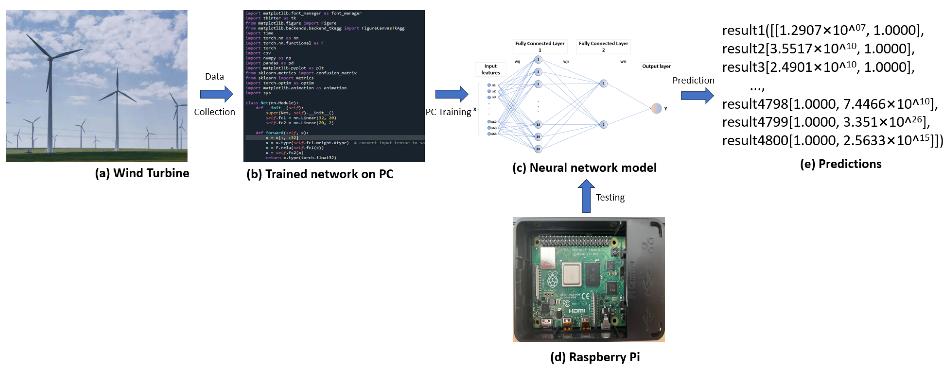
The overview of the proposed method is shown in Figure 1. The vibration signal is collected by accelerometers, which are located at the non-drive end in the wind turbine. Wind turbines are usually constructed in areas where wind energy is abundant, such as coastlines, mountains, plains, and deserts.
Figure 1a shows wind turbines constructed on grasslands. The data were trained in the model, which was implemented in Python language on PC. The data were divided into small segments; thus, the model can quickly analyze each segment without other processing methods, as shown in Figure 1b,c. The trained neural model was embedded in the Raspberry Pi, as is shown in Figure 1d. The last step was for the trained model to predict each segment’s score, as is shown in Figure 1e.
2.2. The Description of the Neural Network Model
Many research works use neural networks for fault detection or the monitoring of bearings. Fu et al. [26] monitored wind turbines with deep learning. In their paper, CNN and LSTM are used to analyze variables and monitor wind turbine gears. Gearbox bearing temperature data are processed for AI monitoring and troubleshooting. Asmuth and Korb [27] provide a basic three-dimensional CNN-based wake model to predict wind turbine wake flow fields. The model accurately predicts wake flow characteristics, showing its potential for wind turbine wake forecasts. Xie et al. [28] proposed an attention mechanism-based CNN-LSTM wind turbine fault prediction model. The CNN extracts features, LSTM captures time sequence correlations, and an attention algorithm gathers fault-related target information from the ontology-annotated Semantic Sensor Network. The model was shown to be precise and generalized.
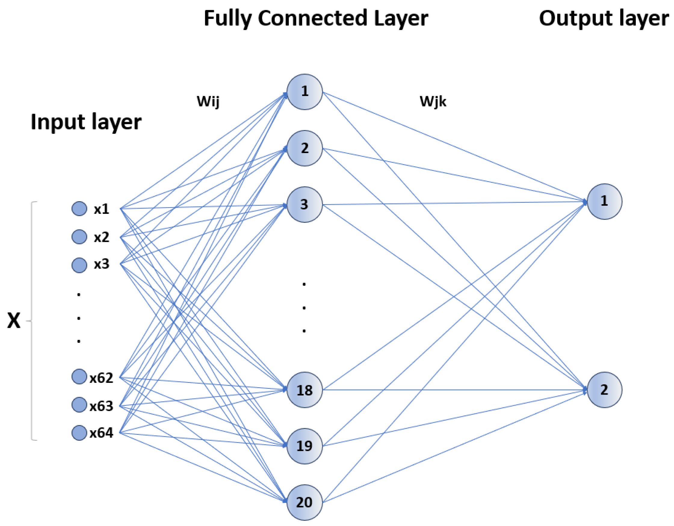
In this paper, we adopted a real-time detection neural network model to assess wind turbine bearing failure, as shown in Figure 2. The model adopts the architecture of a Multi-Layer Perceptron (MLP) [29].
The neural network model contains two fully connected layers (FC1 and FC2), and the second fully connected layer (FC2) acts as the output layer. The first full connected layer (FC1) has 64 input features and 20 hidden units, which are used to learn complex features in the input data. The output layer (FC2) is a layer that takes the 20 output features from FC1 and reduces them to two output features, which are used to map the learned features to faults and normal categories.
2.3. From Input Layer to Hidden Layer
The input vector . The first fully connected layer has a weight matrix and a bias vector . The operation performed by this layer can be expressed as:
Then, the ReLU (Rectified Linear Unit) activation function is applied to h. The ReLU function is defined as , which introduces non-linearity, allowing the model to learn more complex functions:
In the hidden layer of the model, the ReLU (Rectified Linear Unit) [30] is used as the activation function. The ReLU function can enhance the non-linear modeling capabilities of the model and help capture the complex features of the input data.
2.4. From Hidden Layer to Output Layer
The vector is then passed through the output layer (‘FC2’), which transforms the 20-dimensional input into a 2-dimensional output suitable for binary classification. Let the weight matrix of the output layer be and the bias vector be . The final output y can be expressed as:
During the forward-direction of the model, the input data that first passed the first full connection layer (FC1) and activated the function ReLU are applied to the output of the hidden layer. Then, the final prediction result is output through the output layer (FC2).
In order to enable the model to accurately identify the mode of health and bearing faults, the method of monitoring learning was adopted for the training of model parameters. The labeling dataset was used for training and optimizing the weight and bias of the model by minimizing the loss function, so that the prediction results of the model were as close to the real label as possible.
The structure of neural network models is simple and effective, with less parameters and computing complexity, and it can operate efficiently on edge equipment such as a Raspberry Pi. Through this model, we can realize the real-time detection of wind turbine bearing faults and provide fast and accurate predictive results to provide feasible solutions for reducing maintenance costs and improving the availability and efficiency of wind turbines.
2.5. Acceleration Sensor and Data Logger
As shown in Figure 3a, the primary purpose of the acceleration sensor located on the bearing is to monitor and assess the condition and functionality of the bearings. These sensors offer an efficient means for detecting and preventing possible malfunctions by monitoring the acceleration of the vibration in the bearing while it is in operation [31,32,33].
2.6. Raspberry Pi
With Eben Upton serving as the project manager, the “Raspberry Pi Charity Foundation” was established in the UK. The world’s smallest desktop computer, sometimes referred to as a card-type computer, was officially introduced in March 2012 by Emben Apoton [36], a Cambridge University research lab.
3. Experiment
3.1. Dataset
There are many acceleration sensors on the generator bearing of a wind turbine. The data used in the experiment were the signal of one of the acceleration sensors. The data were collected from the turbine generator of a company. The vibration data were collected at 25,600 samples/second and a collection time of 3 s.
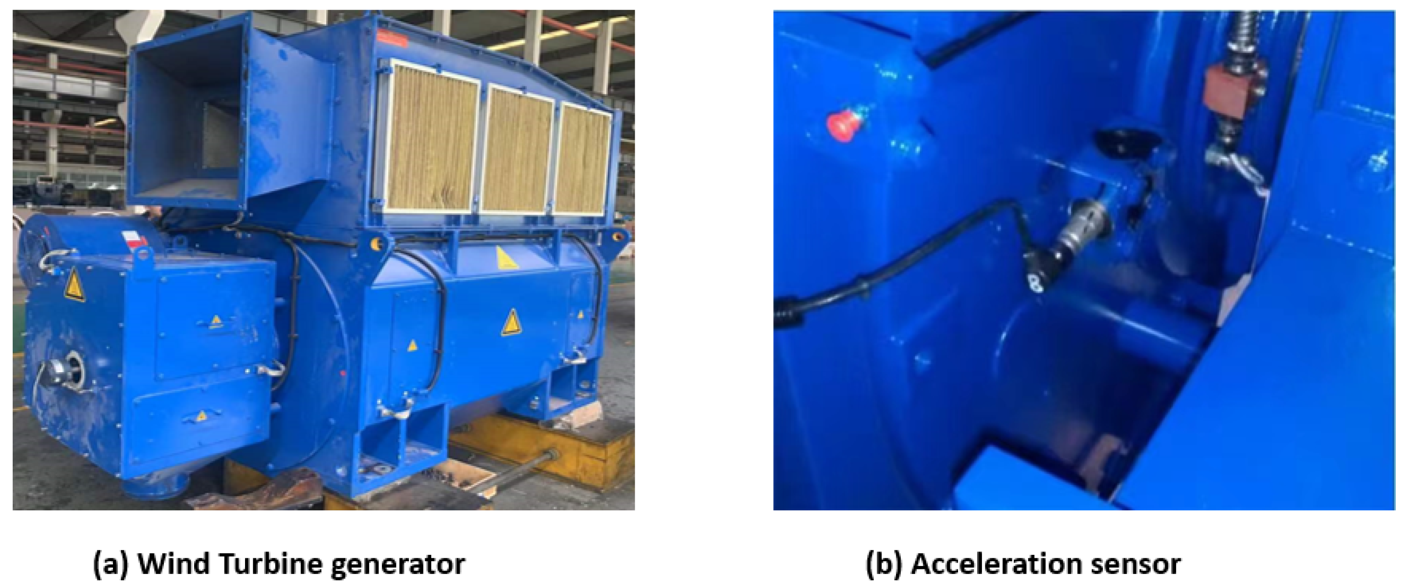
The generator is a device that converts mechanical energy into electrical energy. It usually consists of a rotor and a stator, where the rotor is supported by bearings rotating on a shaft. The generator bearing is an important component that supports the rotor, and its proper functioning is critical to the performance and reliability of the generator. It is shown in Figure 4a.
In order to monitor the health of generator bearings, acceleration sensors are installed on the bearings. An acceleration sensor is a device that measures the acceleration of an object. When a generator is in operation, the bearings are subjected to a variety of forces and vibrations that cause the bearings to change in acceleration. The acceleration sensor senses and measures these changes and converts them into a digital signal. It is shown in Figure 4b.
Important information about generator bearing vibration can be obtained by analyzing the data collected by the acceleration sensor. Vibration data can include parameters such as the vibration amplitude, the frequency, and the time variation. These data are critical for monitoring the health of the bearing. Abnormal vibration data may indicate bearing failure or wear, such as loose bearings, overheating, or damage. By detecting these problems in time, the safety monitoring system can take appropriate repair and maintenance measures to prevent further damage or failure from occurring.
Therefore, acceleration sensor data acquisition is crucial for generator bearing monitoring and maintenance. It provides valuable information to better manage and optimize the generator system, ensuring its proper operation and extended service life.
Two different states are Normal and Fault. Each state has 9600 segments in testing, 2400 segments in training, and each segment has 64 samples; details are shown in Table 1.
3.2. Experimental Setup
3.2.1. Data Analysis
As shown in Figure 5, the length of each sample of raw data was 64, and the raw data produced irregular waveform diagrams. The difference in the amplitude value was readily apparent. After FFT, the difference between health and faults at the peak value was also obvious.
3.2.2. Data Groups
The parameter information is shown in Table 2. The data were evenly divided into 10 groups of data with different states, including five normal states (Group 1–5) and five fault states (Group 6–10). In the experiment, in order to validate the performance of the methodology, comparison models were introduced, i.e., a Medium Neural Network, Wide Neural Network, Bi-layer Neural Network, Tri-layer Neural Network, and Narrow Neural Network. The validation of the method accuracy was determined under 5-fold cross-validation.
3.3. Experimental Results
In this experiment, to verify the performance, five comparison networks were introduced. The first was used to confirm the accuracy of each method and the second was used to confirm the testing time of each method.
3.3.1. Comparison Performance
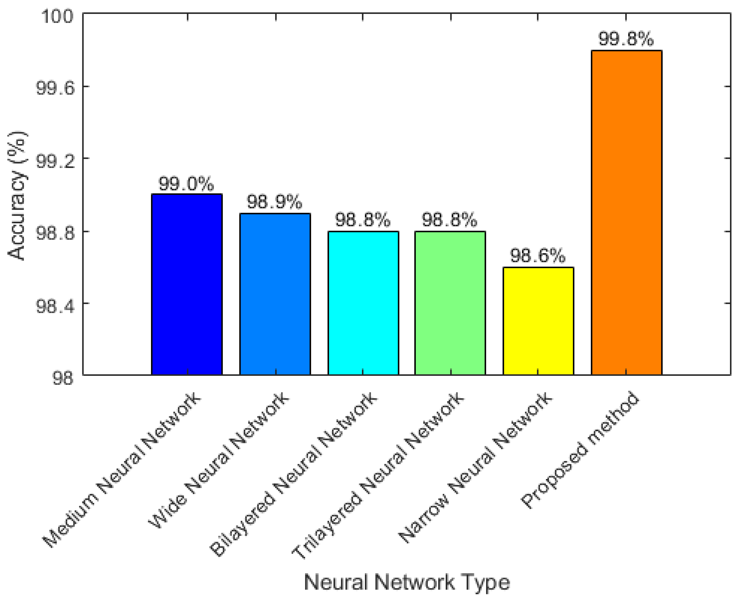
In this part, the raw data were trained and tested with a few neural network methods [38]. For testing the comparison methods, the best method was the Medium Neural Network, whose accuracy was 99.0%. The poorest one was the Narrow Neural Network, whose accuracy was 98.6%. For the proposed method, the accuracy achieved was 99.8%. The accuracy data are shown in Figure 6.
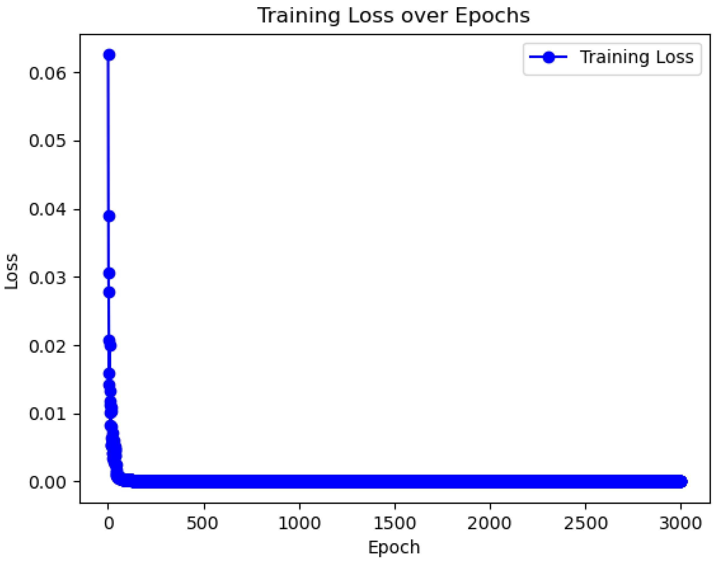
For proposed method, the network output was used to classify tasks (using ‘CrossEntropLoss’). The loss curve of changes with training progress shows that the training converged, as is shown in Figure 7.
3.3.2. Speed
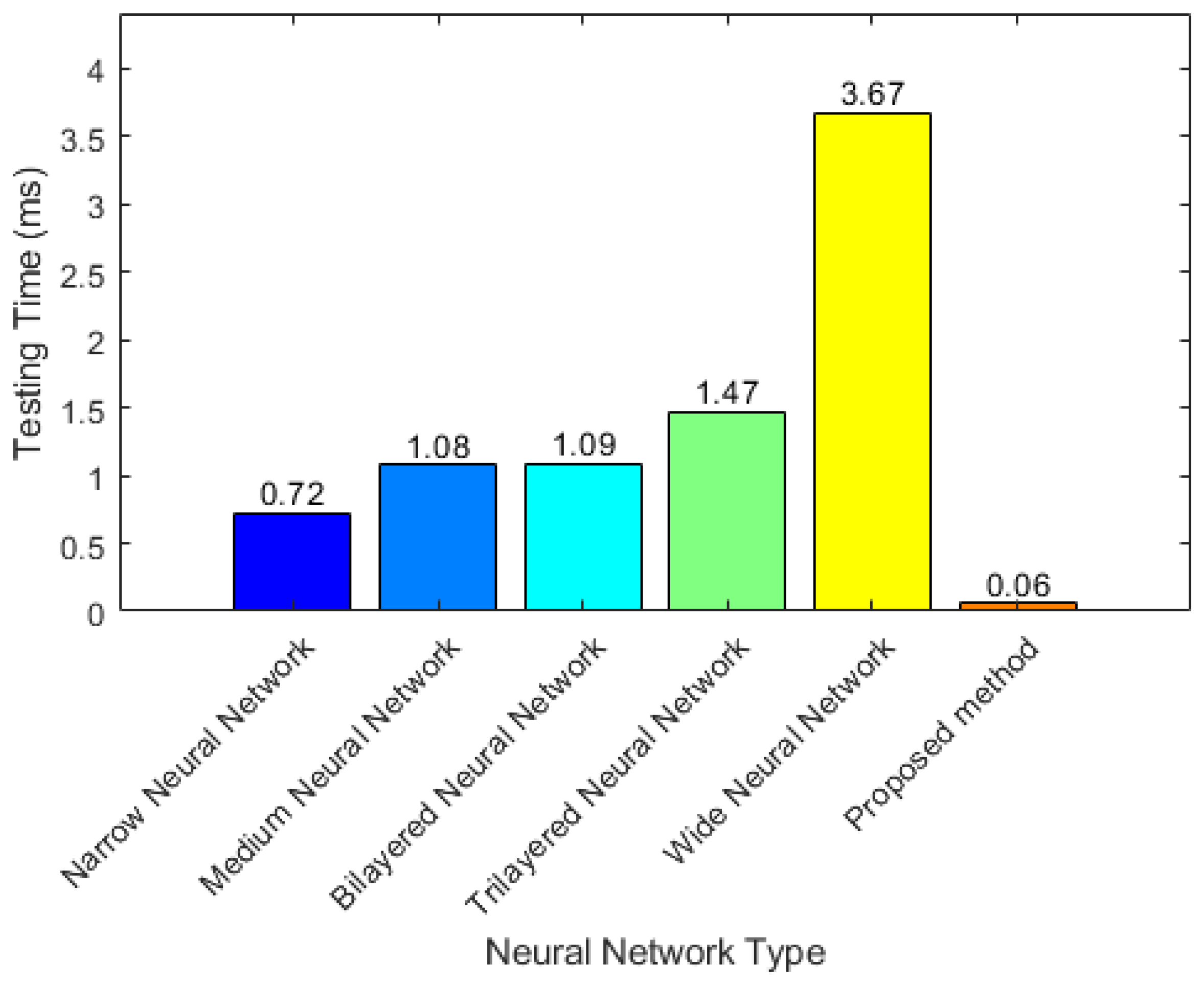
In this part, the tested times are shown in Figure 8. From the five comparison methods, the fastest was the Narrow Neural Network, whose testing time was 0.72 ms. The slowest was the Wide Neural Network, whose testing time was 3.67 ms. For the proposed method, the testing time achieved was 0.06 ms.
For the compared methods, they had a similar accuracy at around 99.0%. However, the testing time of the Wide Neural Network was greater than that of the other methods at 3.67 ms. The main reason for this is that this network has a wide layer. The fastest comparison method was the Narrow Neural Network because of its narrow layer. The average accuracy of the proposed method was 99.8% and the testing time was within 0.06 ms under 5-fold cross-validation. Compared with the other methods, these values represent improvements of 0.8% and 0.66 ms, respectively. It is obvious from the Figure 8 that the proposed method had a better performance than the other methods.
4. Discussion
Achieving a practical model requires a small model, with a high accuracy that can function in real time.
4.1. Effect of Different Segments and Epochs
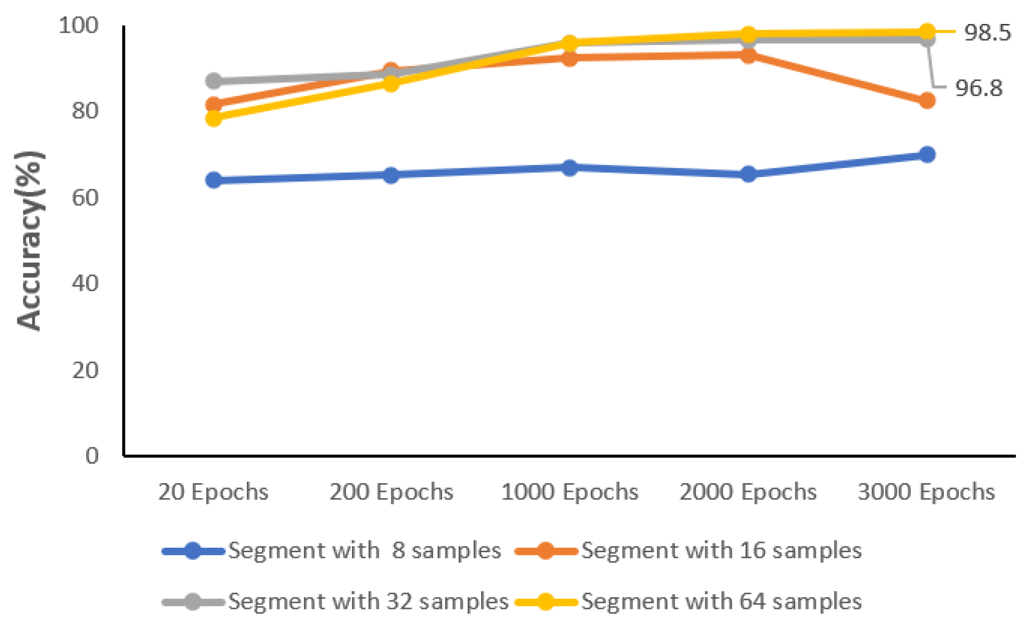
There are four types of segments: the first kind of segment has 8 samples, the second segment has 16 samples, the third segment has 32 samples, and the last segment has 64 samples. In this experiment, different epochs were tested: 20 epochs, 200 epochs, 1000 epochs, 2000 epochs, and 3000 epochs. In addition, the layer size in this experiment was 10. The results are shown in Figure 9.
From Figure 9, the best performance was observed for 32 sample segments and 64 sample segments. Among them, the best results were seen at 3000 epochs. For 32 sample segments, the result was 96.8% and, for 64 sample segments, it was 98.5%. Hence, the segments of 32 and 64 samples at 3000 epochs were tested in the next experiment.
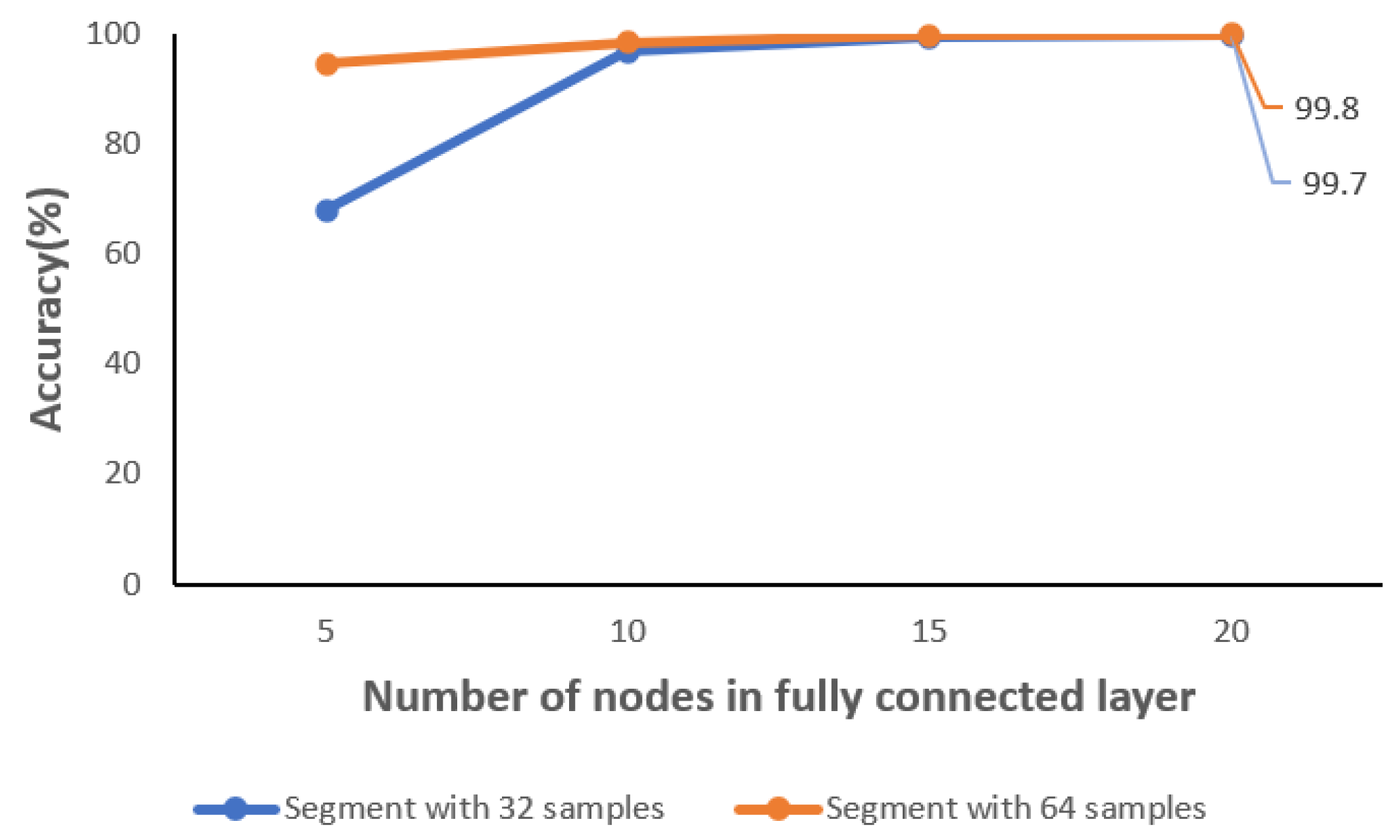
4.2. Effect of Different Number of Nodes
For testing the effect of a different number of nodes in the network, two ablation experiments were introduced. Details are shown in Table 3.
In the first experiment, each of these had 2400 segments, and each segment had 32 samples. Among them, 5-fold cross-validation was applied. Moreover, 19,200 segments were training segments, and the remaining 4800 segments were test segments.
For the second experiment, each of these had 1200 segments, and each segment had 64 samples. Among them, 5-fold cross-validation was applied. Moreover, 9600 segments were training segments, and the remaining 2400 segments were test segments.
In this part, testing was performed with different numbers of nodes, i.e., 5, 10, 15, and 20, in the fully connected layer and at 3000 epochs to validate the model. There were five groups. The final model was obtained through training data and was tested with the remaining data from this model.
As shown in Figure 10, the best performance was obtained for a 20-layer ANN, which achieved 99.8% for 32 samples and 99.7% for 64 samples with a model size of around 5 kb. Therefore, the next step was to confirm the testing time so that the experiment could achieve real-time detection.
4.3. Experiment of Speed
In this part, the length of the layer was 20 and the epoch was 3000. The testing time was tested on different devices: a desktop computer and the Raspberry Pi. The results are shown in Table 4.
On the Raspberry Pi, for 64 samples of segments, the testing data were divided into 2400 segments, and each segment had 64 points.
The proposed system can efficiently process the sensor data and performs rapid analysis and prediction within 0.059 milliseconds per data segment. The experimental results demonstrate that the model achieves a 99.8% accuracy in detecting wind turbine bearing faults within milliseconds of their occurrence.
Regarding the 32 samples per segment, the testing dataset was divided into 4800 individual segments, with each segment consisting of 32 samples. In terms of system performance, the proposed approach exhibits efficient data processing capabilities, enabling swift analysis and prediction within a remarkable timeframe of 0.028 milliseconds per data segment. The experimental findings underscore the model’s exceptional accuracy, with a reported 99.7% detection rate for wind turbine bearing faults within milliseconds of their manifestation.
On the desktop, for 64 samples of segments, the testing data were divided into 2400 segments, and each segment had 64 samples.
The proposed system can efficiently process the sensor data and performs rapid analysis and prediction within 0.009 milliseconds per data segment. The experimental results demonstrate that the model achieves a 99.8% accuracy in detecting wind turbine bearing faults within milliseconds of their occurrence.
In the case of segments consisting of samples, the testing dataset was partitioned into 4800 individual segments, with each segment containing 32 samples. The proposed system demonstrates notable efficiency in processing sensor data, facilitating swift analysis and prediction within an impressive timeframe of 0.005 milliseconds per data segment. The experimental results substantiate the model’s remarkable performance, yielding a detection accuracy of 99.7% in identifying wind turbine bearing faults within milliseconds of their manifestation.
Both the Raspberry Pi and the desktop achieved identical outcomes by utilizing the proposed method. However, the testing times varied. The Raspberry Pi was significantly slower than the PC when it came to test speeds. The proposed method was significantly better, with respect to accuracy and execution time, compared to the comparison networks. The proposed method demonstrated superior performance and aligns with the specific requirements. Multiple models were chosen based on our requirements, i.e., for rapid speed, we selected 32 samples per segment, and for high precision, we chose 64 samples per segment. Each model was approximately 5 kb in size.
5. Conclusions
This study developed a machine learning-based model on a Raspberry Pi to detect wind turbine bearing faults in real time. The model was designed and trained on a desktop computer due to its higher performance. Then, real-time implementation was achieved by running the model on a Raspberry Pi for real-time wind turbine bearing fault detection. The experimental results demonstrate that the model achieves a high accuracy and rapid detection of faults within milliseconds of their occurrence. The model achieved an accuracy rate of 99.8% and the testing time was 0.059 ms, indicating its effectiveness and precision in detecting wind turbine bearing faults.
This study demonstrates the practical implications and potential applications of real-time fault detection in wind turbines using a neural network model. The model provides significant accuracy in quickly identifying bearing faults and providing immediate predictions during fault detection, resulting in reduced maintenance costs, increased turbine availability, and improved overall efficiency. By being able to identify faults during turbine operation in a timely manner, the development of this neural network model facilitates early warning and rapid response, minimizing downtime and associated maintenance costs. Ultimately, real-time fault detection ensures reliable turbine operation and increased availability.
The findings of this study are significant for promoting renewable energy generation and reducing reliance on fossil fuels. The model improves operational efficiency and reliability by enabling the real-time detection of wind turbine bearing faults, minimizing energy waste. This facilitates the wider adoption of renewable energy sources, reducing dependence on finite fossil fuel resources and promoting sustainable energy development and environmental protection.
In the future, many works will require enhancement, and network design optimization will be of paramount importance. This model can only be used on specific models of wind turbines and is restricted to the generator bearings of these turbines. Future research must establish a multi-channel, multi-type, and multi-scenario detection model that can be further optimized to improve the generalizability of models.
Continued innovation and improvement in this area will drive renewable energy generation, reducing dependence on fossil fuels and paving the way for a cleaner, more sustainable energy future.
Author Contributions
Conceptualization, H.M., T.W., R.Q. and F.Z.; methodology, H.M. and T.W.; validation, T.W.; formal analysis, T.W. and R.Q.; investigation, T.W., R.Q. and F.Z.; resources, T.W.; data curation, T.W.; writing—original draft preparation, T.W., R.Q. and F.Z.; writing—review and editing, T.W., H.M. and A.K.N.; supervision, H.M. and T.W.; project administration, H.M. and T.W. All authors have read and agreed to the published version of the manuscript.
Funding
This work was supported in part by the Royal Society award (number IEC\NSFC\223294) to Professor Asoke K. Nandi.
Institutional Review Board Statement
Not applicable.
Informed Consent Statement
Not applicable.
Data Availability Statement
The data presented in this study are available on request from the corresponding author. The data are not publicly available due to commercial privacy.
Conflicts of Interest
The authors declare no conflicts of interest.
References
- IEA. World Energy Outlook 2021. International Energy Agency. 2021. Available online: https://www.iea.org/reports/world-energy-outlook-2021 (accessed on 1 March 2024).
- Ma, J.; Yuan, Y.; Chen, P.; Sitahong, A. Spatiotemporal Attention-Based Long Short-Term Memory Auto-Encoder Network for Early Fault Detection of Wind Turbine Generators. 14 November 2022. Available online: https://www.researchsquare.com/article/rs-2206291/v1 (accessed on 3 April 2024).
- Liao, Y.-H.; Wang, L.; Yan, Y. Instantaneous rotational speed measurement of wind turbine blades using a marker-tracking method. In Proceedings of the 2022 IEEE International Instrumentation and Measurement Technology Conference (I2MTC), Ottawa, ON, Canada, 16–19 May 2022; pp. 1–5. [Google Scholar]
- Wang, M.-H.; Hsieh, C.-C.; Lu, S.-D. Fault diagnosis of wind turbine blades based on chaotic system and extension neural network. Sens. Mater. 2021, 33, 2879–2895. [Google Scholar] [CrossRef]
- Gao, Z.; Liu, X. An overview on fault diagnosis, prognosis and resilient control for wind turbine systems. Processes 2021, 9, 300. [Google Scholar] [CrossRef]
- Liu, W.; Yin, R.; Zhu, P. Deep learning approach for sensor data prediction and sensor fault diagnosis in wind turbine blade. IEEE Access 2022, 10, 117225–117234. [Google Scholar] [CrossRef]
- Pozo, F.; Vidal, Y.; Serrahima, J.M. On real-time fault detection in wind turbines: Sensor selection algorithm and detection time reduction analysis. Energies 2016, 9, 520. [Google Scholar] [CrossRef]
- Zhang, F.; Sun, W.; Wang, H.; Xu, T. Fault diagnosis of a wind turbine gearbox based on improved variational mode algorithm and information entropy. Entropy 2021, 23, 794. [Google Scholar] [CrossRef] [PubMed]
- Ruiz, M.; Mujica, L.E.; Alferez, S.; Acho, L.; Tutiven, C.; Vidal, Y.; Rodellar, J.; Pozo, F. Wind turbine fault detection and classification by means of image texture analysis. Mech. Syst. Signal. Process 2018, 107, 149–167. [Google Scholar] [CrossRef]
- Tang, M.; Chen, Y.; Wu, H.; Zhao, Q.; Long, W.; Sheng, V.S.; Yi, J. Cost-sensitive extremely randomized trees algorithm for online fault detection of wind turbine generators. Front. Energy Res. 2021, 9, 686616. [Google Scholar] [CrossRef]
- Peng, H.; Zhang, H.; Fan, Y.; Shangguan, L.; Yang, Y. A review of research on wind turbine bearings’ failure analysis and fault diagnosis. Lubricants 2022, 11, 14. [Google Scholar] [CrossRef]
- Tian, H.; Fan, H.; Feng, M.; Cao, R.; Li, D. Fault diagnosis of rolling bearing based on hpso algorithm optimized cnn-lstm neural network. Sensors 2023, 23, 6508. [Google Scholar] [CrossRef] [PubMed]
- Khorram, A.; Khalooei, M.; Rezghi, M. End-to-end CNN+ LSTM deep learning approach for bearing fault diagnosis. Appl. Intell. 2021, 51, 736–751. [Google Scholar] [CrossRef]
- Zhang, F.; Zhu, Y.; Zhang, C.; Yu, P.; Li, Q. Abnormality detection method for wind turbine bearings based on CNN-LSTM. Energies 2023, 16, 3291. [Google Scholar] [CrossRef]
- Xu, Z.; Li, C.; Yang, Y. Fault diagnosis of rolling bearing of wind turbines based on the variational mode decomposition and deep convolutional neural networks. Appl. Soft. Comput. 2020, 95, 106515. [Google Scholar] [CrossRef]
- Xu, Z.; Mei, X.; Wang, X.; Yue, M.; Jin, J.; Yang, Y.; Li, C. Fault diagnosis of wind turbine bearing using a multi-scale convolutional neural network with bidirectional long short term memory and weighted majority voting for multi-sensors. Renew. Energy 2022, 182, 615–626. [Google Scholar] [CrossRef]
- Cao, L.; Qian, Z.; Zareipour, H.; Huang, Z.; Zhang, F. Fault diagnosis of wind turbine gearbox based on deep bi-directional long short-term memory under time-varying non-stationary operating conditions. IEEE Access 2019, 7, 155219–155228. [Google Scholar] [CrossRef]
- Khan, P.W.; Yeun, C.Y.; Byun, Y.C. Fault detection of wind turbines using SCADA data and genetic algorithm-based ensemble learning. Eng. Fail. Anal. 2023, 148, 107209. [Google Scholar] [CrossRef]
- Zhao, D.; Wang, T.; Chu, F. Deep convolutional neural network based planet bearing fault classification. Comput. Ind. 2019, 107, 59–66. [Google Scholar] [CrossRef]
- Wang, Z.; Zhu, J.; Gu, J.; Hu, J.; Zhou, B.; Zhao, J. Fault Diagnosis of Wind Turbine Bearing on SATLBO-MLP. In Proceedings of the 2022 China Automation Congress (CAC), Xiamen, China, 25–27 November 2022. [Google Scholar]
- Zhou, Z.; Chen, X.; Li, E.; Zeng, L.; Luo, K.; Zhang, J. Edge intelligence: Paving the last mile of artificial intelligence with edge computing. In Proceedings of the IEEE; IEEE: Piscataway, NJ, USA, 2019; Volume 107, pp. 1738–1762. [Google Scholar] [CrossRef]
- LeCun, Y.; Bengio, Y.; Hinton, G. Deep learning. Nature 2015, 521, 436–444. [Google Scholar] [CrossRef] [PubMed]
- Goodfellow, I.; Bengio, Y.; Courville, A. Deep Learning; MIT Press: Cambridge, MA, USA, 2016. [Google Scholar]
- Lipton, Z.C.; Berkowitz, J.; Elkan, C. A critical review of recurrent neural networks for sequence learning. arXiv 2015, arXiv:1506.00019. [Google Scholar]
- Schmidhuber, J. Deep learning in neural networks: An overview. Neural Netw. 2015, 61, 85–117. [Google Scholar] [CrossRef]
- Fu, J.; Chu, J.; Guo, P.; Chen, Z. Condition monitoring of wind turbine gearbox bearing based on deep learning model. IEEE Access 2019, 7, 57078–57087. [Google Scholar] [CrossRef]
- Asmuth, H.; Korb, H. WakeNet 0.1-A simple three-dimensional wake model based on convolutional neural networks. J. Phys. Conf. Ser. 2022, 2265, 22066. [Google Scholar] [CrossRef]
- Xie, Y.; Zhao, J.; Qiang, B.; Mi, L.; Tang, C.; Li, L. Attention mechanism-based CNN-LSTM model for wind turbine fault prediction using SSN ontology annotation. Wirel. Commun. Mob. Comput. 2021, 2021, 6627588. [Google Scholar] [CrossRef]
- Kruse, R.; Mostaghim, S.; Borgelt, C.; Braune, C.; Steinbrecher, M. Multi-layer perceptrons. In Computational Intelligence: A Methodological Introduction; Springer: Berlin/Heidelberg, Germany, 2022; pp. 53–124. [Google Scholar]
- He, J.; Li, L.; Xu, J.; Zheng, C. ReLU deep neural networks and linear finite elements. arXiv 2018, arXiv:1807.03973. [Google Scholar]
- Bao, M.H. Micro Mechanical Transducers: Pressure Sensors, Accelerometers and Gyroscopes; Elsevier: Amsterdam, The Netherlands, 2000. [Google Scholar]
- Denishev, K.H.; Petrova, M.R. Accelerometer design. In Proceedings of the Electronics 2007, Sozopol, Bulgaria, 19–21 September 2007; pp. 159–164. [Google Scholar]
- Vetelino, J.; Reghu, A. Introduction to Sensors; CRC Press: Piscataway, NJ, USA, 2017. [Google Scholar]
- Park, J.; Mackay, S. Practical Data Acquisition for Instrumentation and Control Systems; Newnes: Oxford, UK, 2003. [Google Scholar]
- Emilio, M.D.P. Data Acquisition Systems; Springer: Cham, Switzerland, 2013. [Google Scholar]
- Severance, C. Eben upton: Raspberry pi. Computer 2013, 46, 14–16. [Google Scholar] [CrossRef]
- Pajankar, A. Raspberry Pi Image Processing Programming: With NumPy, SciPy, Matplotlib, and OpenCV; Apress: New York, NY, USA, 2022. [Google Scholar]
- Selvi, M.S.; Rani, S.J. Classification of admission data using classification learner toolbox. J. Phys. Conf. Ser. 2021, 1979, 12043. [Google Scholar] [CrossRef]
Figure 1.
Overview of the system: (a) wind turbine; (b) modeling in python language; (c) neural network model; (d) Raspberry Pi implementation; and (e) predictions.
Figure 1.
Overview of the system: (a) wind turbine; (b) modeling in python language; (c) neural network model; (d) Raspberry Pi implementation; and (e) predictions.

Figure 2.
Proposed network.

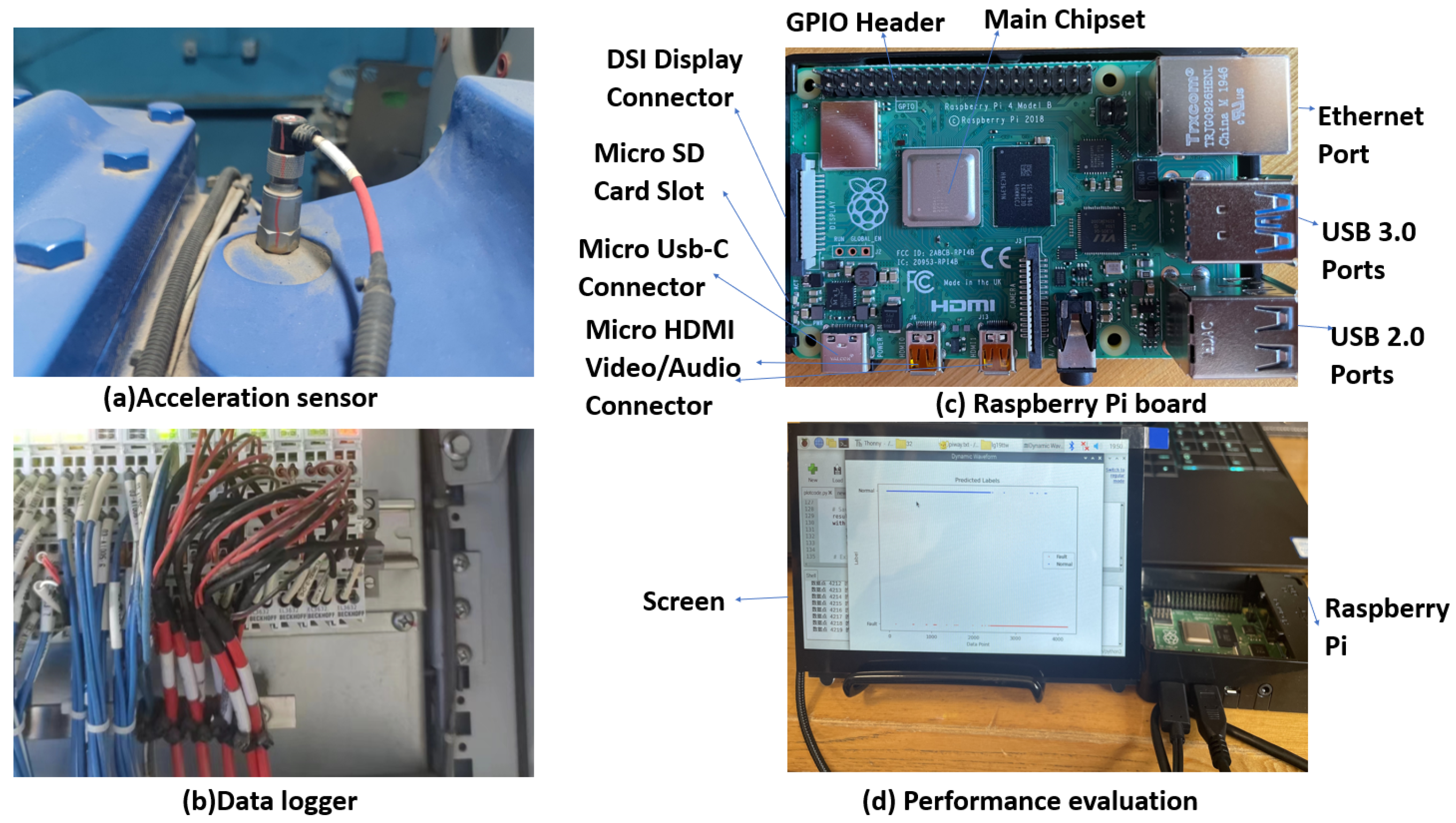
Figure 3.
(a) Acceleration sensor, (b) data logger, (c) Raspberry Pi board, and (d) performance evaluation.
Figure 3.
(a) Acceleration sensor, (b) data logger, (c) Raspberry Pi board, and (d) performance evaluation.

Figure 4.
Data collection platform. (a) Wind turbine generator; (b) acceleration sensor.

Figure 5.
Data spectrum.

Figure 6.
Comparison of accuracy of raw data.

Figure 7.
The loss curve of changes with training progress.

Figure 8.
Comparison of testing time of raw data.

Figure 9.
Accuracy of different samples in each segment.

Figure 10.
Accuracy under different numbers of nodes in the fully connected layer.


Table 1.
Description of data.
| Fault Type | Training Segments | Testing Segments | Samples in Each Segment |
|---|---|---|---|
| Normal | 9600 | 2400 | 64 |
| Fault | 9600 | 2400 | 64 |
Table 2.
Dataset was split into training and testing subsets.
| Training Group | Testing Group | ||
|---|---|---|---|
| Subset 1 | 2, 7, 3, 8, 4, 9, 5, 10 | Subset 1 | 1, 6 |
| Subset 2 | 1, 6, 3, 8, 4, 9, 5, 10 | Subset 2 | 2, 7 |
| Subset 3 | 1, 6, 2, 7, 4, 9, 5, 10 | Subset 3 | 3, 8 |
| Subset 4 | 1, 6, 2, 7, 3, 8, 5, 10 | Subset 4 | 4, 9 |
| Subset 5 | 1, 6, 2, 7, 3, 8, 4, 9 | Subset 5 | 5, 10 |
Table 3.
Description of different segments.
| Samples in Each Segment | Fault Type | Training Segments | Testing Segments |
|---|---|---|---|
| 32 | Normal | 19,200 | 4800 |
| Fault | 19,200 | 4800 | |
| 64 | Normal | 9600 | 2400 |
| Fault | 9600 | 2400 |
Table 4.
Test results and time of raw data on Raspberry Pi and desktop computer.
| Samples of Segment | Devices | Accuracy | Testing Time | Sampling Time |
|---|---|---|---|---|
| 32 | Desktop | 99.8% | 0.009 ms | 2.5 ms |
| Raspberry Pi | 99.8% | 0.059 ms | ||
| 64 | Desktop | 99.7% | 0.005 ms | 1.25 ms |
| Raspberry Pi | 99.7% | 0.028 ms |
Disclaimer/Publisher’s Note: The statements, opinions and data contained in all publications are solely those of the individual author(s) and contributor(s) and not of MDPI and/or the editor(s). MDPI and/or the editor(s) disclaim responsibility for any injury to people or property resulting from any ideas, methods, instructions or products referred to in the content. |
© 2024 by the authors. Licensee MDPI, Basel, Switzerland. This article is an open access article distributed under the terms and conditions of the Creative Commons Attribution (CC BY) license (https://creativecommons.org/licenses/by/4.0/).
Share and Cite
MDPI and ACS Style
Wang, T.; Meng, H.; Qin, R.; Zhang, F.; Nandi, A.K. Real-Time Monitoring of Wind Turbine Bearing Using Simple Neural Network on Raspberry Pi. Appl. Sci. 2024, 14, 3129. https://doi.org/10.3390/app14073129
AMA Style
Wang T, Meng H, Qin R, Zhang F, Nandi AK. Real-Time Monitoring of Wind Turbine Bearing Using Simple Neural Network on Raspberry Pi. Applied Sciences. 2024; 14(7):3129. https://doi.org/10.3390/app14073129
Chicago/Turabian StyleWang, Tianhao, Hongying Meng, Rui Qin, Fan Zhang, and Asoke Kumar Nandi. 2024. "Real-Time Monitoring of Wind Turbine Bearing Using Simple Neural Network on Raspberry Pi" Applied Sciences 14, no. 7: 3129. https://doi.org/10.3390/app14073129
Note that from the first issue of 2016, this journal uses article numbers instead of page numbers. See further details here.