Abstract
Black soil plays an important role in maintaining a healthy ecosystem, promoting high-yield and efficient agricultural production, and conserving soil resources. In this paper, a typical black soil area of Keshan Farm in Qiqihar City, Heilongjiang Province, China, is used as a case study to investigate the black soil farmland productivity evaluation model. Based on the analysis of the composite index (CI) model, productivity index (PI) model and various machine learning models, the soil productivity evaluation method was improved and a prediction model was established. The results showed that the support vector machine regression model based on simulated annealing algorithm (SA-SVR), as well as the Gaussian process regression model (GPR), had obvious advantages in data preprocessing, feature selection, and model optimization compared to the modified composite index model (MCI), the modified productivity index model (MPI), and the coefficients of determination (R2) of their modelling, which were up to 0.70 and 0.71, respectively, and these machine learning prediction models can reflect the effects on maize cultivation and its yield through soil parameters even with small datasets, which can better capture the nonlinear relationship and improve the accuracy and stability of yield prediction, and is an effective method for guiding agricultural production as well as soil productivity evaluation.
1. Introduction
The world population is expected to reach 9 × 109 by 2050, and in response to this demographic pressure, the demand for world food production will increase by 60–70 percent [1,2]. Land is a fundamental resource for food production [3], and its quality and productivity are directly related to food supply and national economic stability. Although it is widely recognized that soil is an abundant resource, the reality is that soil resources are being rapidly degraded due to salinization, erosion, compaction, pollution, structural collapse, acidification, organic matter, biological activities, and urban and industrial development [4]. It is necessary to study soil productivity evaluation methods to maintain soil productivity, and finding more effective assessment methods by studying land productivity is essential to improve agricultural production efficiency and promote sustainable agriculture. Research on land productivity evaluation is conducted to gain a comprehensive understanding of land fertility, potential, and its adaptability under different environmental conditions, to support scientific and rational land management, to better plan agricultural production, to reduce pressure on land resources, and to promote the maintenance of ecological balance.
Land productivity evaluation methods in past studies relied on laboratory analyses and statistical methods, mainly CI models [5] as well as PI models [6]. Gao Chang et al. [7] summarized the methods related to land productivity evaluation and achieved some results in assessing soil fertility and potential in China; Duan Xingwu et al. [8] improved the PI model based on PI model applied to the dry-hot valleys in China; El-Nady MA [9] confirmed that the PI model is a good prediction model for maize yield; Yang Z et al. [10] used an improved soil productivity index model to study the process of soil productivity change in post-dam debris flow sediments during the restoration process; however, these research methods are mainly for estimating land productivity, and their final derived land productivity indices are closely related to the observed areas [11]. Although there are advanced methods for uncertainty treatment of estimation, such as the National Commodity Crop Productivity Index (NCCPI) [12], there are always limitations in the estimation of land productivity assessment methods, which rely on the scores given by the experts’ experience or the choice of parameter values in the function when constructing the affiliation function in the process of data processing and modelling.
Since traditional farming methods are characterized by excessive allocations, which have significant economic and environmental impacts [13], agricultural management requires accurate estimation of land productivity, determination of various combinations of soil composition and nutrient precision to analyze the soil to reduce the cost of cultivation. Machine learning models can effectively avoid this evaluation uncertainty caused by empirical knowledge and subjective judgement, and by learning from soil data, assessment models can be built more quickly and accurately. Zhou et al. [14] used a combination of optical and radar remote sensing data to apply the SVM algorithm to build a Soil organic C (SOC) prediction model; Zou et al. [15] collected historical soil data from southern China and combined multivariate linear model (MLM) and mixed effects regression model (MEM) for soil productivity assessment; Shehu et al. [16] obtained 1781 sets of maize farmland data comparison in Northern Nigeria using linear regression models, as well as random forest machine learning to predict maize yields based on nutrient concentrations in spike leaves; Pan Y et al. [17] provided an estimate of land productivity in the conterminous United States of America (CONUS) through machine learning algorithms using a data-driven approach to incorporate relationships from the data into the land productivity evaluation. However, challenges remain in terms of applicability and interpretability of machine learning models [18], including the requirement of datasets (e.g., combining large remote sensing datasets and larger historical datasets) and due to the black box nature of machine learning resulting in little insight into agricultural management.
In order to address these limitations, this paper studies land productivity evaluation methods using the black soil area of Northeast China as a case study, and compares and optimizes land productivity evaluation learning methods to improve the performance and explanatory ability of the model. By making full use of the soil data acquired by the group, an accurate and reliable land productivity evaluation model is established. The purpose of this study is to establish a reasonable land productivity evaluation model based on the field scale through the case of land productivity evaluation methods in the black soil area of Northeast China, the data set of these models contains only the physicochemical properties of the soil, and in order to ensure the validity of the data set the soil selection blocks of this group are basically at a similar altitude and the same slope. This kind of evaluation method can inspire the relationship between soil and crop in other regions, such as the county level, and provide a scientific basis for national and regional agricultural decision-making.
2. Materials and Methods
2.1. Data Sources and Data Preprocessing
2.1.1. Description of the Experimental Site
The data in this paper were obtained from Keshan Farm in Qiqihar City, Heilongjiang Province, China, which is located in the territory of Nehe and Keshan County, at 48°12′–48°23′ N, 125°8′–125°37′ E. Its land area is about 351 square kilometers (km2), and the cultivated area is about 272 km2. The farmland’s landscape is primarily characterized by rolling hills and undulating terrains. It is located on the western foothills of the Lesser Khingan Mountains and in the northeastern part of the Songnen Plain. The slopes generally range from 1 to 5 degrees, with an average slope of 3 degrees. The length of slopes is mostly between 500 and 100 m. The average altitude is 315 m. The annual average temperature is 1.3 °C. The main climatic characteristics in spring are windy with sparse rainfall, while summer is primarily characterized by concentrated and heavy rainfall. Winter temperatures are cold, with a lowest temperature of −37.6 °C, and snowfall is the primary form of precipitation. The soil of Keshan Farm is mainly black calcareous soil, belonging to the typical black soil region of Northeast China.
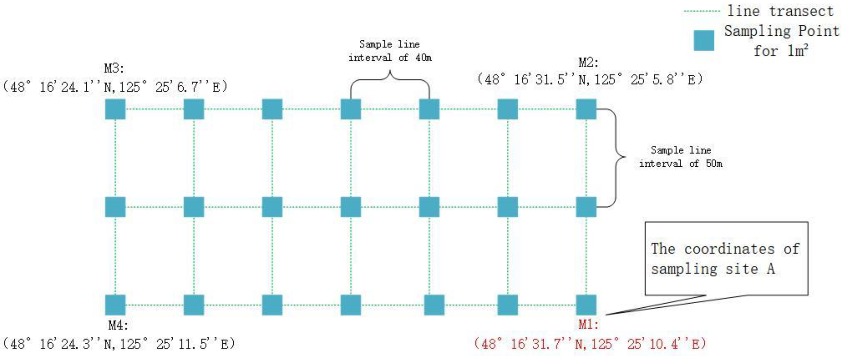
In October 2022, the research team selected Sample Plot A (48°16′31.7″ N, 125°25′10.4″ E) in Keshan Farm, which had been reclaimed for 26 years. In this area, 21 field sampling points were obtained. Sample Plot B (48°16′37.7″ N, 125°25′4.6″ E), reclaimed for 39 years, yielded 15 field sampling points. Sample Plot C (48°17′0.0″ N, 125°24′6.4″ E), reclaimed for 59 years, provided 45 field sampling points. Lastly, Sample Plot D (48°21′12.5″ N, 125°33′5.3″ E), reclaimed for 90 years, contributed 33 sampling points. In total, 114 soil physicochemical data points and corresponding yield data were collected. The sampling methods were identical across all four plots, and a schematic diagram of the sampling process in Sample Plot A is shown in Figure 1.

Figure 1.
Schematic diagram of the distribution of 21 sampling points in Plot A.
2.1.2. Measurement of Physical and Chemical Properties of Soil
Fresh fruits were harvested within a 1 square meter area centered on the sampling point for maize yield measurement. Threshed fruits were weighed, and the yield was calculated based on a moisture content of 14%. Soil sampling was conducted with the sampling point as the center, collecting topsoil samples (0–5 cm) using a soil auger.
The measurement of soil physical indicators includes bulk density and moisture content. Bulk density was determined using the ring knife method [19,20], and moisture content was measured using the drying method [19,20].
Soil chemical indicators were measured, including total nitrogen, total carbon, total phosphorus, total potassium, alkali nitrogen, available phosphorus, available potassium, and pH. Measurement methods involved acid-base elimination for total nitrogen, total carbon, total phosphorus, and total potassium. Soil samples were digested under acidic and alkaline conditions, followed by measuring the respective element contents [21,22,23]. Alkali nitrogen, available phosphorus, and available potassium were measured using alkali extraction, strong acid extraction, and weak acid extraction methods, respectively [21,22,23]. pH was measured using a soil-to-water ratio of 2.5:1. Each indicator was replicated three times, and the average was taken.
2.1.3. Data Preprocessing
In this study, data pre-processing was applied to ensure that the soil productivity evaluation model achieved excellent performance in terms of accuracy and stability. Specific methods employed include the 3σ principle, box-and-line plot analysis, Z-score normalization, outlier removal, and L2 feature selection. Outliers in the dataset were identified and removed by the 3σ principle and box-and-line plot analysis to eliminate anomalous data points that might be caused by measurement errors, data entry errors, or other reasons. In order to address the differences in different feature scales, a Z-score normalization method was used to transform the data for each feature into a standard normal distribution with mean 0 and standard deviation 1, ensuring that all features have equal weights in the model.
In order to improve model performance, it is necessary to obtain important features from a large number of input features. The benefit of reducing the feature dimension is that it reduces the risk of overfitting while improving the model performance [24]. Among multiple feature selection methods, we compare the advantages of different methods and combine them with the characteristics of the data in this study; L1 feature selection, L2 feature selection, and PCA dimensionality reduction are more effective. L1 feature selection and L2 feature selection are regularization methods in machine learning; L1 feature selection tends to make the weight of some features zero through L1 regularization (Lasso), achieving sparsity in feature selection. L2 feature selection, on the other hand, uses L2 regularization (Ridge), which tends to smooth out the weights by penalizing the sum of the squares of the model parameters, but does not make them zero. PCA dimensionality reduction method maps the original features to a new low-dimensional space by finding the principal components in the data. PCA differs from L1 and L2 in that it does not focus exclusively on the target variable, but rather on selecting the principal components by maximizing the data variance to select principal components. In the experimental results L2 feature selection works best with the small dataset of this study. The advantage of L2 feature selection is that it is more robust to covariate data, helps to deal with the presence of highly correlated features without being easily over-influenced by specific features, and improves the stability and generalization ability of the model.
2.2. Topsoil Productivity Evaluation Model
In this section, we present detailed methods commonly used to estimate land productivity evaluation models, optimized for the location where the samples were collected for this project; the focus will be on two specific models: the Modified Composite Index (MCI) model, and the Modified Topsoil Productivity Index (MPI) model.
2.2.1. CI Model and Its Revisions
The CI model, namely the Comprehensive Index model, is a surface soil assessment method established on the foundation of soil productivity coefficients proposed by Shuying Leng et al. [5]. This method comprehensively considers multiple key factors, including the content of organic matter, available nitrogen, available phosphorus, available potassium, soil acidity and alkalinity, soil texture, erosion status, and topography, encompassing eight aspects in total.
The content of organic matter, available nitrogen, available phosphorus, and available potassium in the surface soil reflects the nutrient status of the soil, while soil acidity and alkalinity, soil texture, erosion status, and topography involve the physical properties and geographical environment of the soil. These eight factors are considered crucial in influencing land productivity. By comprehensively considering them, the CI model provides a holistic productivity assessment for the soil. The scores for each factor can be obtained from relevant literature and expert experiences. The summation of these scores constitutes the comprehensive index of the CI model, where higher scores indicate a greater contribution to soil productivity (Table 1).

Table 1.
Soil impact factor score sheet.
Surface soil productivity index is evaluated using the following indicators:
In the formula, CI represents the Soil Productivity Index, where i takes values from 1 to 8, representing the eight considered factors. Xi denotes the weights assigned to the eight selected factors, and Yi represents the scores for these eight factors. The topographical factor ‘a’ is not considered in the formula due to the uniformity of maize soil sampling within the same farm.
Taking into account the importance of soil physicochemical indicators in the production of maize crops in Northeast Black Soil and the accessibility of relevant data, we have chosen the indicators of Soil Alkaline Nitrogen (A), Available Phosphorus (B), Available Potassium (C), Suitability Index for pH value (D), Moisture Content (E), and Soil Bulk Density (F) for the original surface soil assessment model. The weights assigned to these indicators in the original model are 10%, 10%, 10%, 20%, 20%, and 20%, respectively.
The analyses yielded a ration of A:B:C:D:E:F = 1:1:1:2:2:2 for these indicators, highlighting their equal importance in the overall soil productivity assessment. Considering that these assessments were carried out on the same farm, we ignored possible climatic influences from different regions. As a result, the resulting Modified Composite Index (MCI) model was obtained as follows:
This allocation strategy reflects the importance of each of the selected indicators, taking into account their joint influence in the overall soil productivity assessment of the black soil zone in northeastern China.
2.2.2. PI Model and Its Revisions
The PI model was first proposed by Neill [6] in 1979 to assess the effect of soil properties on crop yield. It has been modified by some researchers in the past [25,26,27]. On the basis of Duan Xingwu’s improved PI model, the special case of organic matter and soil bulk density in the black soil area of Northeast China was considered, and the growth of maize was taken as an example [28]. The optimized PI model was established by dividing the soil depth of 200 cm into 20 layers and selecting the soil physicochemical indicators [6] The soil physico-chemical indexes were selected to establish PI model:
In the formula, PI represents the Soil Productivity Index, where i denotes different soil layers. As this study focuses on the surface soil productivity assessment method, deeper soil layers are not considered. Nevertheless, it is essential to understand that, in the formula, A represents the Suitability Index of soil available water content for root growth, B represents the Suitability Index of soil aeration for root growth, C represents the Suitability Index of soil bulk density for root growth, D represents the Suitability Index of soil pH for root growth, E represents the Suitability Index of soil electrical conductivity for root growth, and WF represents the root weight factor of the soil. Each suitability index is standardized to a numerical value between 0.000 and 1.000, with values closer to 0 indicating inhibition of crop growth and values closer to 1 indicating suitability for crop growth.
Referring to the research by Pierce [26], three key indicators were selected, namely the Suitability Index of soil available water content (A), Suitability Index of soil bulk density (C), and Suitability Index of soil pH (D).
The calculation formula for the Suitability Index of soil available water content refers to the research findings of scholars such as Grossman [29], providing an improvement to the surface soil evaluation:
In the equation, A represents the Suitability Index of soil available water content, where AWC represents the soil’s available water content expressed in volume percentage. The calculation is based on field capacity and wilting point humidity.
The Suitability Index of soil pH (D) refers to the calculation formula proposed by Pierce [26], with improvements made for surface soil assessment:
The soil bulk density calculation method is consistent with the approach used in Duan Xingwu’s modified PI model [27].
Considering the critical nature of soil physicochemical property indicators in maize crop production in Keshan Farm, this study was revised based on the PI model. In order to assess the surface condition of the soil more accurately, we evaluated only the top soil layer of the ploughed soil. On the basis of retaining the original soil pH suitability index D, water content A and soil bulk weight C, we added the total nitrogen index B, quick-acting phosphorus index E, and quick-acting potassium index F, and constructed a modified PI model (MPI) applicable to the evaluation of topsoil:
Multiple parameters of the soil have a differential effect on the overall fertility level, and the measured values of each parameter have significant differences in magnitude, making a simple summation calculation impossible. To overcome this problem, a standardized approach is used in this paper.
When the measured value of a parameter belongs to the “poor” grade, i.e., P ≤ Xa:
When the measured value of a parameter falls within the “qualified” grade, i.e., Xa < P ≤ Xb:
When the measured value of a parameter belongs to the “medium” grade, i.e., Xb < P ≤ Xc:
When the measured value of a parameter belongs to the “good” grade, i.e., Xc < P ≤ Xd:
When the measured value of a parameter belongs to the “excellent” grade, i.e., Xd < P:
In the above formulae, E represents the quality index of available phosphorus (P) in the soil, P denotes the measured value of soil available phosphorus, and Xa, Xb, Xc, and Xd are the grading standard values. By employing this standardization method, the single quality indexes of the same level attribute become more comparable, enhancing comparability. When the measured value (P) exceeds the optimal standard (Xd), the single quality index (E) no longer increases, reflecting that the crop (corn) does not necessarily benefit from higher soil attribute values. In other words, after reaching a certain optimal level of nutrient content, further fertilization to increase content does not contribute to increased crop yield.
Based on this, the optimized evaluation formula for the soil available phosphorus quality index E in this experiment is as follows:
Based on the soil evaluation score formulated by Leng Shuying [15], we further subdivided the total nitrogen quality index and available potassium quality index in the soil to ensure that the actual scores fall within the range of 0 to 1, in accordance with the requirements of the PI model. In the end, we obtained the calculation formulas for the total nitrogen index (B) and available potassium index (F):
The subdivision and standardization methods contribute to a more accurate quantification of the impact of total nitrogen and available potassium on soil nutrient conditions. This optimization of surface soil assessment aligns with the design principles of the PI model.
2.3. Machine Learning Model Selection and Its Optimization
In this section, the selection of machine learning models will be illustrated, and then the details of the three machine learning models selected for soil productivity evaluation in this paper will be presented: a support vector machine regression model based on simulated annealing algorithm (SA-SVR), a Gaussian process regression (GPR), and a multilayer perceptron combined with random forest regression (MLP-RFR), where SA-SVR and MLP-RFR will be compared with their classical models SVR and RFR to show their optimization justification in Section 3.2 (Performance Analysis of Machine Learning Models), where a comparison of results with their classical models, SVR and RFR, will be made to show the reasonableness of their optimization. Each technique will be explained. This includes their respective characteristics in the context of yield prediction, describing the operation of training and optimizing each model using the dataset.
2.3.1. Machine Learning Model Selection
With the development of machine learning algorithms applied to agricultural prediction models with increasing accuracy, Extreme Gradient Boosting (XGboost), decision tree regression, Long Short-Term Memory (LSTM) regression, SVR, GPR, and random forest regression (RFR) are the methods that have been proven to be more effective [30,31,32,33].
XGboost is a gradient boosting algorithm that is highly flexible and accurate, performs well with large-scale data and complex features, is able to handle nonlinear relationships, and is robust to missing values. Decision Tree is an intuitive and easy to explain algorithm with a strong ability to fit non-linear relationships between features, and is computationally fast compared to other algorithms. LSTM model is a deep learning model for time series data that captures long-term dependencies in time series and performs well for datasets with memory properties. However, XGboost, Decision Tree and LSTM models are sensitive to the overfitting problem on small datasets, and their performance on small datasets is unstable, where Decision Tree is susceptible to the effects of noise and local features in the data, and the LSTM model usually requires a large amount of data for training, which is a long training time compared with traditional machine learning algorithms.
The three methods, SVR, GPR and RFR, have some advantages in targeting the small dataset containing soil physicochemical properties and yield in this experiment. SVM is able to deal with high dimensional data and non-linear relationships, has a strong generalization ability for small sample datasets and has some advantages in controlling model complexity. GPR is a non-parametric model that can flexibly adapt to the data and provides an estimate of prediction uncertainty, which is advantageous for modelling small data sets. Random Forest is an integrated learning algorithm that performs well for noisy data and datasets with complex relationships. It is also relatively robust to feature selection and missing values.
For this study, the three methods of SVR, GPR and RFR are more suitable for constructing accurate prediction models, which can effectively control the complexity of the model when dealing with small datasets, and have better stability and generalization ability.
2.3.2. Support Vector Machine (SVM) Model and Its Optimization
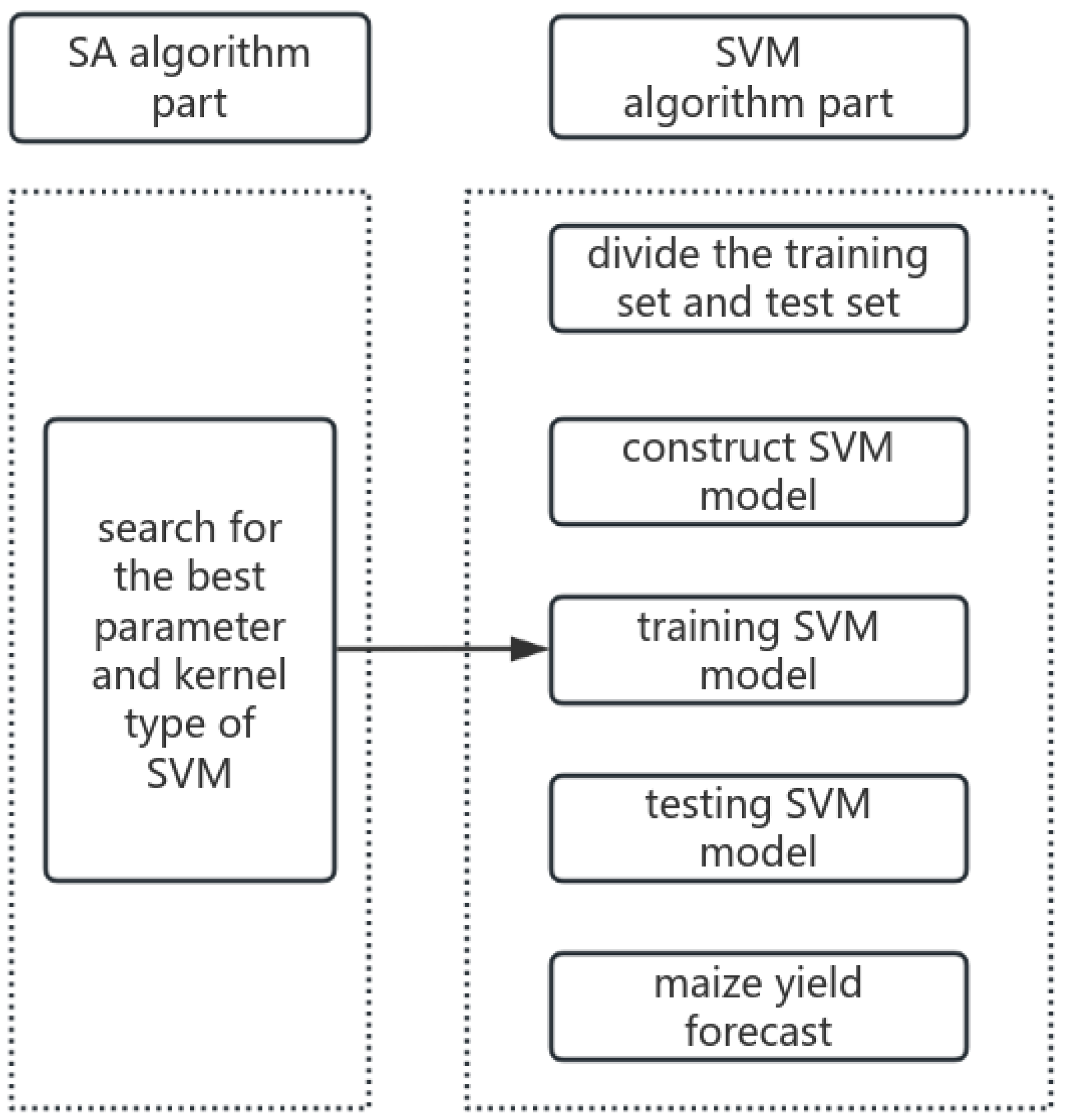
SVM is a powerful machine learning model for regression and classification tasks. In this study, we propose a regression prediction model based on a simulated annealing algorithm to optimize the hyperparameters of the support vector machine, as well as the type of kernel function: the SA-SVM (Figure 2).
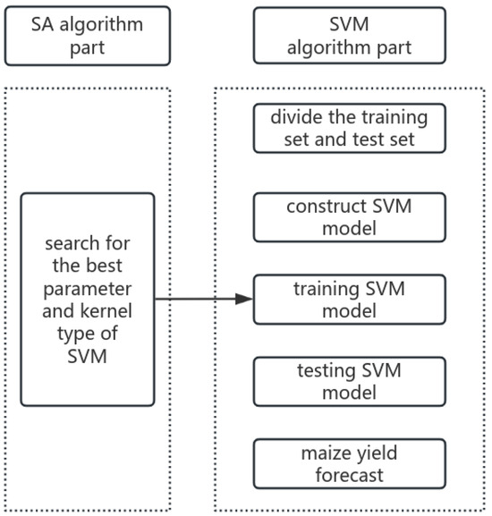
Figure 2.
SA-SVM regression prediction flow chart.
The traditional SVM model constructs several different types of kernel functions based on non-linear sample datasets. It involves training samples with input features and iteratively adjusting parameters until optimal performance is achieved. The selection of an appropriate kernel function is a crucial step in SVM model development. In our approach, we use the Radial Basis Function (RBF) kernel. To prevent overfitting and balance the model’s fit and complexity, we introduce a regularization parameter C. However, the traditional SVM model is time-consuming during parameter tuning, and the obtained result may be a local optimum. Additionally, different kernel function types can impact parameter settings, influencing the performance of the kernel function. After exploring various optimization algorithms, we opted for the Simulated Annealing (SA) algorithm to optimize SVM model parameters. SA is a global optimization algorithm that searches for the optimal combination of hyperparameters, kernel function parameters, and regularization parameter C in the parameter space to enhance the model’s performance. The optimization objective of the SA algorithm is to minimize the loss function, representing the error between the model-predicted yield and the actual yield.
2.3.3. Gaussian Process Regression (GPR) Model
The GPR model is a powerful non-parametric Bayesian regression method. The model is based on a Gaussian process that maps the input space to the output space and expresses the prediction uncertainty in the form of a probability distribution. The core idea is to infer the output values of new data points and their uncertainty by modelling the similarity between training data points. The mean function is usually assumed to be zero or learnt from the data. The covariance function defines the relationship and correlation between different input points. Given the mean and covariance functions, GPR models the objective function as a Gaussian distribution. When new input points are predicted, GPR provides a predicted posterior distribution of possible function values, including the predicted mean and variance for each point [30]. For the small dataset of this study, the number of iterations was set to 100. One of the strengths of the GPR model is its flexibility and versatility to adapt to a variety of complex nonlinear relationships. Due to the nonparametric nature of the Gaussian process, the model does not require a pre-specified functional form, performs well with small samples of data, and is suitable for the experimental design of this topic.
2.3.4. Random Forest Regression (RFR) Model and Its Optimization
The RFR model is a popular machine learning algorithm that allows higher accuracy results in various fields, including crop yield prediction [34,35]. The RFR model improves the prediction performance by constructing the integration of multiple decision trees to effectively mitigate the overfitting problem. Each tree is trained on the basis of random subsamples and random features, and finally the results of each tree are integrated through a voting mechanism, which improves the generalization ability of the model and robustness to outliers. Multilayer Perceptron with Random Forest Regression (MLP-RFR) is an innovative model that has received much research attention in recent years [36]. As a flexible neural network model, the multilayer perceptron (MLP) improves the performance of the model by adjusting the number of layers and nodes in the hidden layer, and selecting appropriate activation functions (e.g., sigmoid, tanh, Relu, etc.) and loss functions (e.g., mean-square error, cross-entropy, etc.). The MLP-RFR model combines the multilayer perceptron’s (MLP’s) non-linear modeling ability and the Random Forest. The integrated learning mechanism of the MLP overcomes the dependence of traditional neural networks on a large amount of labelled data by embedding the MLP into a Random Forest, and performs well in small sample data scenarios.
These methods were applied to a comprehensive dataset containing 87 sets of data. This dataset covered 10 physical and chemical properties of the soil (specific physical and chemical properties can be found in Table 2) and 87 sets of actual values of maize yield. The 10 physicochemical properties of the dataset were used as variables (x) and the actual yields were used as target variables (y). For effective model training and performance evaluation, these data were divided into an 80% training set and a 20% test set, with the random number set to 42 [37]. The trained model was applied on the test set, and the error between the model predicted yield and the actual yield was calculated.
Table 2.
Raw data section table.
2.4. Model Evaluation Criteria
In order to comprehensively assess the performance of the various classical models and their improved models, the following statistics were used to evaluate the prediction results: Mean Square Error (MSE), Mean Absolute Error (MAE), and the Coefficient of Determination (R2) were used as performance indicators to validate the accuracy and adaptability of the models.
Mean Squared Error (MSE) is a commonly used metric to gauge the performance of the model in predicting corn yields. This metric calculates the average squared deviation between the model’s predicted values and the actual yields. By squaring the prediction errors for each data point and then averaging them, MSE provides an overall measure of the model’s prediction errors across all data points. A smaller MSE value indicates that the model’s predictions are closer to the actual values, signifying better predictive performance.
Mean Absolute Error (MAE) is another key metric used to measure the predictive accuracy of the model. In this study, MAE calculates the average absolute error between the actual and predicted corn yields for each data point, offering an overall assessment of the model’s accuracy in yield prediction.
Coefficient of Determination (R2) is an indicator of model explanatory power, representing the proportion of the target variable’s variance that the model can explain. A higher R2 value indicates that the model can better fit the predicted values of corn yield to the actual yields.
3. Results and Analysis
3.1. Performance Analysis of MCI Model and MPI Model
In order to explore the effect of different nutrient factors on soil fertility, the results of MCI and MPI models were used to carry out the study of land productivity index. MCI and MPI models are mainly used to process the different nutrient values of soil samples in a dimensionless and standardized way, and then the data can be calculated by using the two productivity evaluation models (Equations (2) and (6)) to obtain the soil productivity index of each sample. Part of the original data, as shown in Table 2 for the eight sampling points of 10 soil physical and chemical indicators and the actual yield of corn, correspond to the MCI model calculation results. As shown in Table 3, the MCI model shown in the calculation of the results varied from 0.778 to 0.878; the average of all the MCI model calculations of the results in 0.827, corresponding to Table 2 of the MPI model calculations of the results of the MPI model. As shown in Table 4, MPI model calculated results vary from 0.225 to 0.912, and the average of all MPI model calculations is 0.651.
Table 3.
MCI model data processing part of the table.
Table 4.
MPI model data processing part of the table.
The land productivity evaluation index obtained in this study is positively correlated with maize yield, and the larger interval of variation of the productivity index obtained from the calculation indicates that it is more reflective of the difference in actual yields, which indicates the high accuracy of the corresponding results, suggesting that the study has a certain degree of rationality.
In order to deeply study the rationality of maize land productivity evaluation indices on different sampling points, maize yields on different sampling points were collected in the study, and the productivity indices of MCI and MPI models were analyzed by linear regression with the maize yields obtained from the surveys. The results of MCI are shown in Figure 3a, and the results of MPI are shown in Figure 3b; the coefficient of determination of the MPI model, which was improved and applied to topsoil evaluation, reached 0.38 and MSE was 1146.29; the coefficient of determination of the MCI model was 0.23, and MSE was 3589.19. The results showed that both had good linear correlation. The MPI model achieved a coefficient of determination of 0.38 with an MSE of 1146.29, while the MCI model had a coefficient of determination of 0.23 with an MSE of 3589.19. The results showed that both of them had a good linear correlation. Compared with the CI model, which mainly relies on the experience of experts, the improved PI model (MPI) in this experiment has better R2 and MSE indexes, which better reflect the relationship between soil and crop.
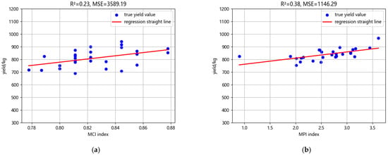
Figure 3.
Correlation graph between traditional improved model evaluation results and yield. (a) Correlation graph between MCI model productivity evaluation results and maize yield. (b) Correlation graph between MPI model productivity evaluation results and maize yield.
3.2. Performance Analysis of Machine Learning Models
Multiple machine learning models were selected for optimal training for regression prediction and compared, including the SVR model (Figure 4a), SA-SVR model (Figure 4b), GPR model (Figure 5), RFR model (Figure 6a), and MLP-RFR model (Figure 6b).
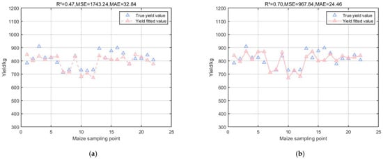
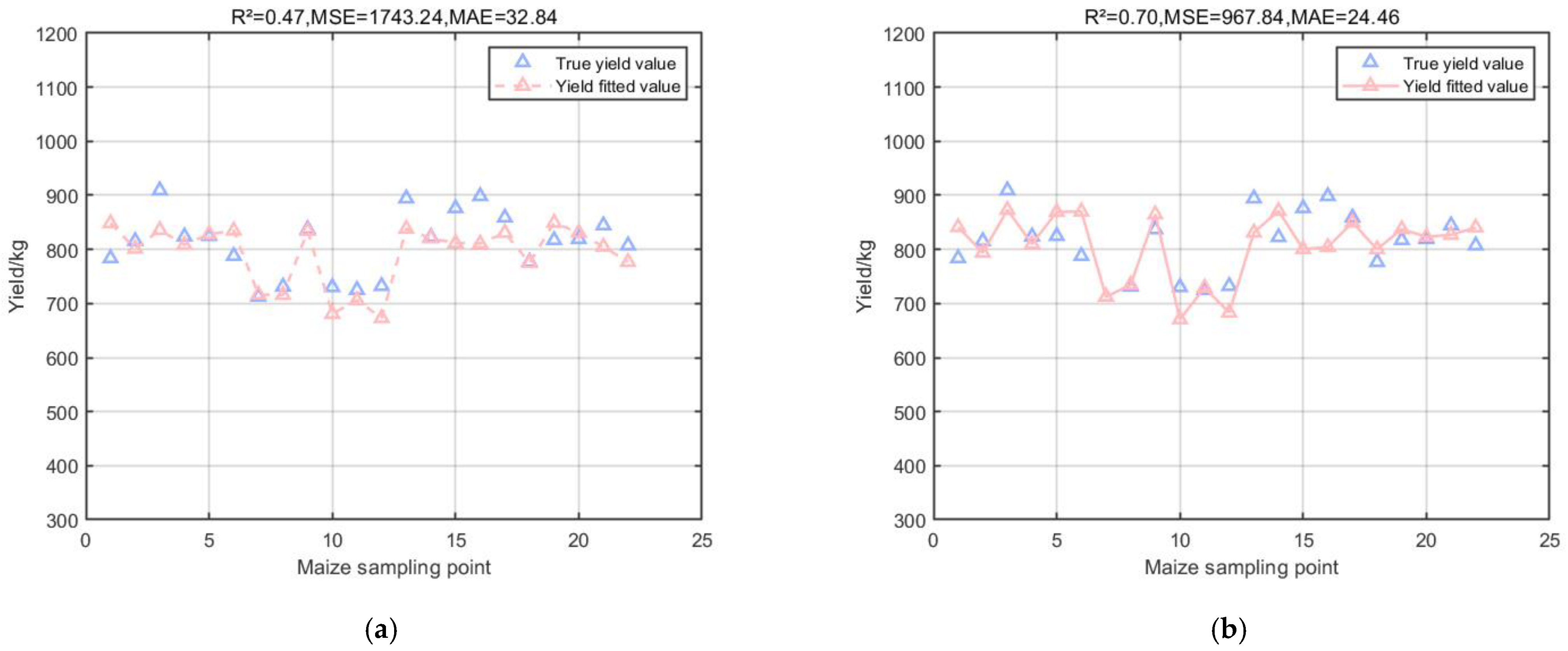
Figure 4.
Results of SVM model and its modified model. (a) Multiple regression results of SVR model on corn yield. (b) Multiple regression results of SA-SVR model on corn yield.
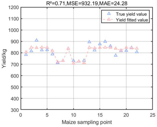
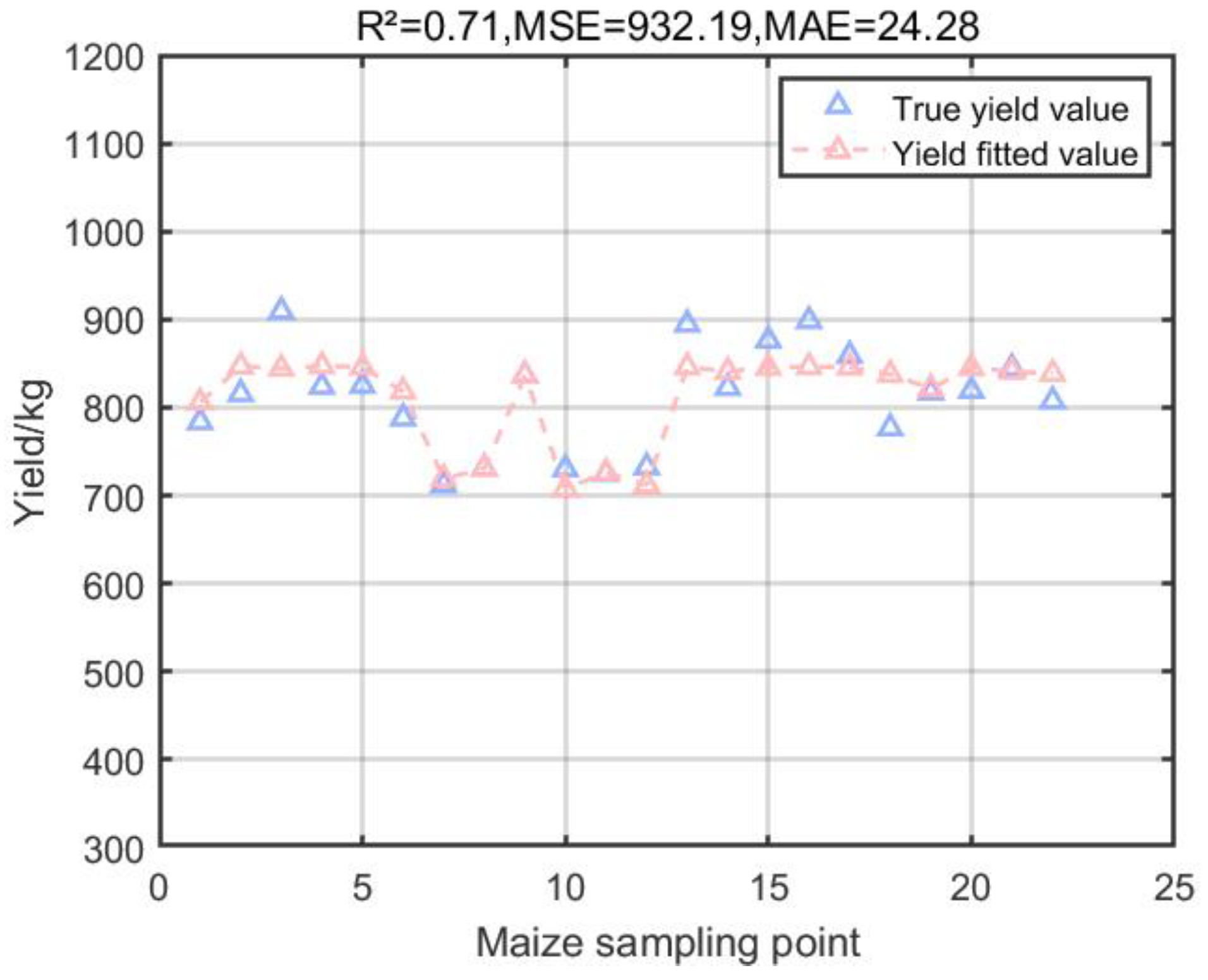
Figure 5.
Multiple regression results of GPR model on corn yield.
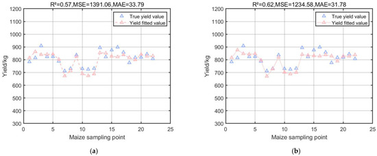
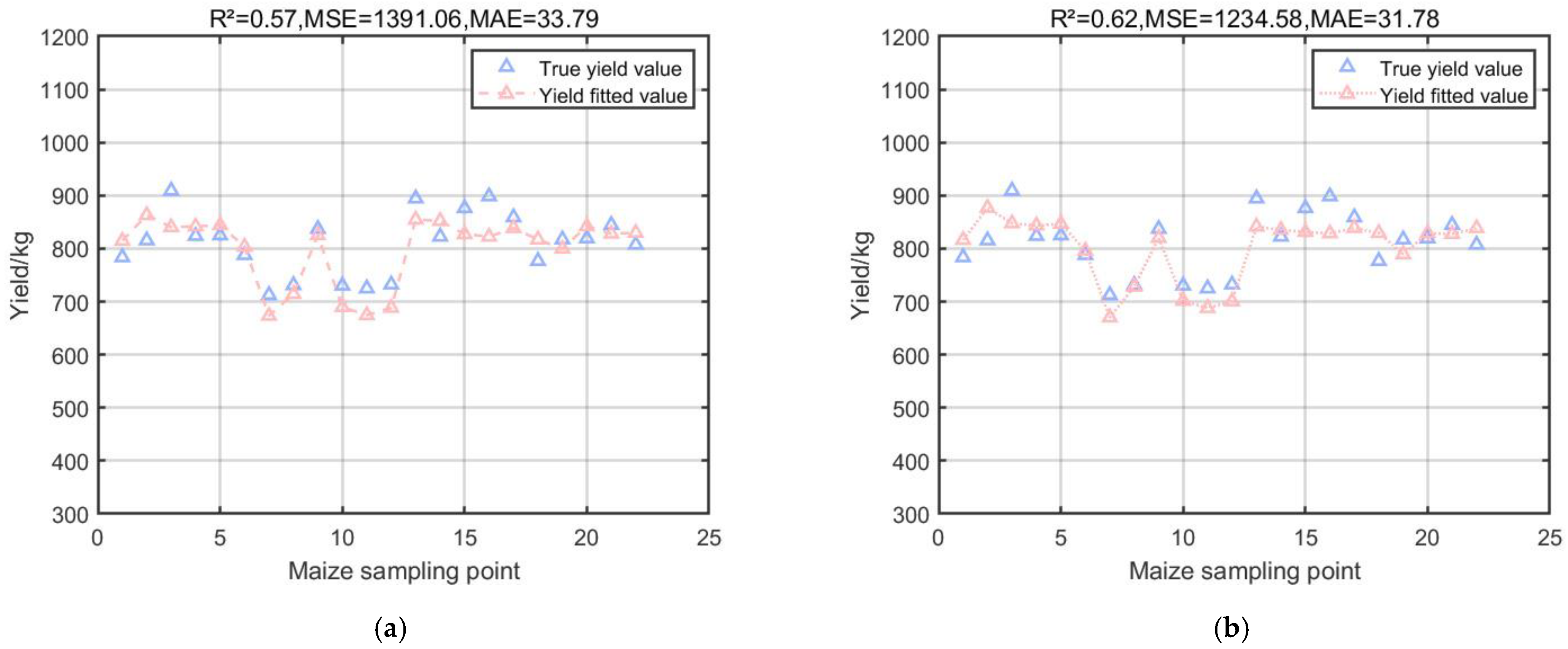
Figure 6.
Results of RF model and its modified model. (a) Multiple regression results of RFR model on corn yield. (b) Multiple regression results of MLF-RFR model on corn yield.
Figure 4a shows that the coefficient of determination R2 of the SVR model is 0.47, which is an improvement compared to the MPI model, but the MSE reaches 1743.24, which indicates that there is a large error when applying it to the test set to predict some of the yields; Figure 4b shows that the coefficient of determination R2 of the SA-SVR model, which combines the SA algorithm, is 0.70, and the MSE decreases to 967.84. The SA algorithm optimizes the minimization loss function which, in this experiment, is specifically shown to effectively reduce the error between the predicted and actual yields in the prediction model. The SA algorithm optimizes the minimization loss function which, in this experiment, effectively reduces the error between the predicted yield and the actual yield in the prediction model; Figure 5 shows that the coefficient of determination R2 of the GPR model is 0.71, and the MSE is 932.19, which is excellent for the small dataset of the experiment due to the nonparametric nature of the GPR model that does not require the function to be pre-specified; and Figure 6a shows that the coefficient of determination R2 of the RFR model is 0.71, and the MSE is 932.19. The coefficient of determination R2 of the RFR model is 0.57, and the MSE is 1391.06, which is also good for the small dataset with complex relationships in this experiment, and the prediction is more reliable than that of the MPI model; Figure 6b shows that the RFR model combined with the MLP can reduce the error by choosing the appropriate activation function and the loss function, and it is applied to the small dataset of the present experiment with the performance of MLP. The coefficient of determination R2 of the RFR model is 0.62, which is improved compared with the RFR model, and the MSE is reduced from 1391.06 to 1234.58 compared with the RFR model.
3.3. Comparison of Model Performance
By comparing the MCI model, the MPI model, the SVR model, the SA-SVR model, the GPR model, the RFR model, and the MLP-RFR model, it is possible to derive specific results regarding the performance of these models (Table 5).
Table 5.
Table of evaluation indicators for linear regression analysis.
The results show that the machine learning models trained through multiple selection and optimization have significant advantages over MCI and MPI models for data processing and prediction in land productivity evaluation. Specifically, we can see that the coefficients of determination (R2) of the machine learning models for yield prediction are higher than that of the MPI model (0.38), especially for the GPR model (0.71), followed by the SA-SVM model (0.70), and the MLP-RFR (0.62), which indicates that the prediction models are more reliable in practical applications, and that the Mean Squared Error (MSE) and Mean Absolute Error (MAE) of the machine learning models are higher than those of the MPI model (0.38). MSE and Mean Absolute Error (MAE) were also significantly improved compared to the MPI model, with the MSE of the GPR model decreasing to 932.19 compared to the MPI model’s 1146.29, and the MSE of the SA-SVR model decreasing to 967.84 compared to the MPI model’s 1146.29. It is clear from these data that the machine learning model has a good performance with multiple soil physicochemical properties as multi-feature inputs, can better handle nonlinear relationships, and can improve the accuracy of yield prediction. At the same time, the limitations of MCI and MPI modeling, which inevitably have subjectivity, were overcome. Moreover, the machine learning algorithm can achieve better soil productivity evaluation results by selecting data and adjusting model parameters in practical applications [38].
4. Discussion
In this paper, we take the black soil area in Northeast China as a case study for land productivity evaluation methodology. In this study, we have thoroughly investigated the performance of different soil productivity evaluation models, including the MCI model, the MPI model, and a variety of classical machine learning models and their optimization models.
The MCI model, after data pre-processing such as 3σ principle, box-and-line diagram and Z-score, can provide a preliminary soil productivity estimation, applicable to the situation of limited data, but cannot deal with the non-linear relationship, and is not sensitive enough to high-dimensional data and complex features. The performance of the MPI model has been improved in relation to the traditional PI model, which can more comprehensively take into account the nature of the soil and the environmental factors, and has a better performance in yield prediction relative to the MCI model (Figure 3), and a more comprehensive performance on complex relationship between soil and crops. The MPI model is more suitable for multifactorial soil productivity evaluation. However, the MPI model is still unable to deal with non-linear relationships and high-dimensional data.
The data in Table 5 indicate that the machine learning models have advantages over the MCI model, as well as the MPI model, in terms of feature selection and model optimization. Based on the results of model performance analysis, SA optimization was chosen to effectively solve the problems of SVM model regarding computational resources and tuning time, and the SVM model searches for the optimal hyperparameters by combining the SA algorithm [38]; the MLP-RFR model effectively mitigates the overfitting problem of complex data patterns and has better robustness to outliers by combining the advantages of MLP and RF. These models can better capture the complex relationship between nonlinear soils and crops.
Previous studies on land productivity evaluation often used machine learning algorithms to build predictive models, mainly by combining a large number of remote sensing data and public historical datasets [32,39,40,41,42], which has the advantage that a large amount of data can be applied to train a predictive model with a high degree of accuracy, but these predictive models generally have regional limitations [11]. The land productivity evaluation method studied in this paper still performs well when applied to a small dataset containing only soil physicochemical properties, with significant improvements in R2, MSE, and other indicators compared to the MCI model as well as the MPI model; as an example, in Table 5 of this study, the SVR model, SA-SVR model, GPR model, RFR model, and the MLP-RFR model studied have improved R2 compared to the MPI model with an improved R2, indicating that soil variables are closely related to yield and can effectively predict yield. Despite the investment of significant manpower in collecting samples from the field and determining their specific soil physicochemical properties in the laboratory for this dataset, our research on land productivity evaluation, using black soil in Northeast China as a case study and based on the field scale, has demonstrated the effectiveness of this research method through its prediction accuracy when applied to small datasets. When applied to other regional farmlands, it is only necessary to obtain a small dataset containing the specific physical and chemical properties of the soil and the corresponding yield, and then we can go to a more accurate prediction of the yield of the block of farmland, to verify that the modelling method studied in this experiment for the linkage of the complex relationship between the soil and the crop and, at the same time, we can also evaluate the nutrient deficiencies of the regional soils. Incorporating this research approach into soil management practices and land productivity assessment has great potential to improve agricultural outcomes, promote sustainable development and optimize resource use.
This paper also has some limitations in the study of land productivity evaluation methods; for example, in front of an experienced expert who has studied soil in a region for decades, the land productivity estimation method given by the region will be more accurate [28], which cannot be achieved by using only a small dataset of trained models. Alternatively, the method of this study did not consider the climatic factors due to the block, and although the slope and elevation are guaranteed to be similar when obtaining the physicochemical properties of agricultural soils, it may be necessary to take into account factors such as elevation slope when applying to other regions such as the block size at the county level, which this study does not do at the present time. Although the research on land productivity evaluation methods in this paper is limited, our method of studying soil–crop relationships based on small datasets at the field scale is generalizable and can be tried to be applied to soil–crop relationship problems in other regions [13].
5. Conclusions
This paper focuses on land productivity evaluation methods using black soil farmland blocks in northeast China as a case study, even in the common case where the available dataset is small. The method is applied and validated in the specific case of maize cultivation. The application of the CI model as well as the PI model for soil productivity evaluation was optimized and improved to the MCI model as well as the MPI model by field conditions. The machine learning algorithms were selected with full consideration and optimization of small datasets, including SVM model, SA-SVM model, GPR model, RFR model, and MLP-RFR model, in order to study the accuracy and adaptability of soil productivity evaluation. Based on 10 basic factors such as soil parameters and their nutrient contents, a series of prediction models were established, which used soil physicochemical properties as characteristic inputs and predicted corn yield. From the model performance comparison in Table 5, we can see that the various models can better represent the correlation between soil and crop, which verifies the validity of the methodology of this study. The same research idea can be attempted whenever small datasets are available and the models need to be optimized to improve the accuracy of prediction.
Despite the progress made in this study, there is still room for further exploration. Future research can further improve the accuracy and reliability of soil productivity evaluation by deeply investigating other machine learning methods and deep learning models. Meanwhile, factors not covered in this study such as altitude climate, soil erodibility and other conditions can also be attempted as feature inputs combined with machine learning algorithms for productivity evaluation methodology to enhance the generalizability of the research methodology and further improve the model performance.
Author Contributions
Conceptualization, Y.X. and Z.Z.; methodology, Y.X.; software, Z.Z.; validation, Y.X.; formal analysis, Z.Z.; investigation, Y.X.; resources, Y.X.; data curation, Z.Z.; writing—original draft preparation, Z.Z.; writing—review and editing, Y.X.; visualization, Z.Z.; supervision, Y.X.; project administration, Y.X.; funding acquisition, Y.X. All authors have read and agreed to the published version of the manuscript.
Funding
This research was funded by the National Key Research and Development Program of China (2021YFD1500705).
Institutional Review Board Statement
Not applicable.
Informed Consent Statement
Not applicable.
Data Availability Statement
The data presented in this study are available upon request from the corresponding authors. The data are not publicly available due to privacy.
Acknowledgments
The authors thank the anonymous reviewers for their useful comments, which improved the quality of the paper.
Conflicts of Interest
The authors declare no conflicts of interest. The funders had no role in the design of the study; in the collection, analyses, or interpretation of data; in the writing of the manuscript; or in the decision to publish the results.
References
- Bahuguna, R.N.; Jagadish, K.S.V.; Coast, O.; Wassmann, R. Plant abiotic stress: Temperature extremes. Encycl. Agric. Food Syst. 2014, 4, 330–334. [Google Scholar]
- Saiz-Rubio, V.; Rovira-Más, F. From smart farming towards agriculture 5.0: A review on crop data management. Agronomy 2020, 10, 207. [Google Scholar] [CrossRef]
- Food and Agriculture Organization of the United Nations (FAO). Healthy Soils are the Basis for Healthy Food Production. In Fact Sheet; FAO: Rome, Italy, 2015. [Google Scholar]
- Stupar, V.; Živković, Z.; Stevanović, A.; Stojićević, D.; Sekulić, T.; Bošković, J.Ž.; Popović, V.M. The effect of fertility control on soil conservation as a basic resource of sustainable agriculture. Not. Bot. Horti Agrobot. Cluj-Napoca 2024, 52, 13389. [Google Scholar] [CrossRef]
- Leng, S. Research on the Potential Agricultural I Productivity of China with the Help of Gis. J. Nat. Resour. 1992, 7, 71–79. [Google Scholar]
- Neill, L.L. An Evaluation of Soil Productivity Based on Root Growth and Water Depletion; University of Missouri: Columbia, SC, USA, 1979. [Google Scholar]
- Gao, C.; Li, L.; Zhang, Y. Current advance on soil productivity evaluation. J. Henan Agric. Sci. 2013, 42, 14–18. [Google Scholar]
- Duan, X.W.; Han, X.; Hu, J.M.; Feng, D.T.; Rong, L. A novel model to assess soil productivity in the dry-hot valleys of China. J. Mt. Sci. 2017, 14, 705–715. [Google Scholar] [CrossRef]
- El-Nady, M.A. Evaluation of the productivity of two soils using productivity index. Egypt. J. Soil Sci. 2015, 55, 171–184. [Google Scholar]
- Yang, Z.; Rong, L.; Huang, J.; Duan, X.; Zhang, L.; Liu, J. Response of soil productivity to rehabilitation time in debris flow deposits behind check dams in Hunshui Gully, southwestern China. Arch. Agron. Soil Sci. 2022, 68, 476–487. [Google Scholar] [CrossRef]
- Schaetzl, R.J.; Krist, F.J., Jr.; Miller, B.A. A taxonomically based ordinal estimate of soil productivity for landscape-scale analyses. Soil Sci. 2012, 177, 288–299. [Google Scholar] [CrossRef]
- Dobos, R.; Sinclair, H.; Hipple, K. National Commodity Crop Productivity Index (NCCPI) User Guide v2. 0; USDA NRCS National Soil Survey Center: Lincoln, NE, USA, 2012. [Google Scholar]
- Amani, M.A.; Marinello, F.J.A. A deep learning-based model to reduce costs and increase productivity in the case of small datasets: A case study in cotton cultivation. Agriculture 2022, 12, 267. [Google Scholar] [CrossRef]
- Zhou, Y.; Zhao, X.; Guo, X.; Li, Y. Mapping of soil organic carbon using machine learning models: Combination of optical and radar remote sensing data. Soil Sci. Soc. Am. J. 2022, 86, 293–310. [Google Scholar] [CrossRef]
- Zou, G.; Li, Y.; Huang, T.; Liu, D.L.; Herridge, D.; Wu, J.J.A.J. A Mixed-Effects Regression Modeling Approach for Evaluating Paddy Soil Productivity. Soil Sci. Soc. Am. J. 2017, 109, 2302–2311. [Google Scholar] [CrossRef]
- Shehu, B.M.; Garba, I.I.; Jibrin, J.M.; Kamara, A.Y.; Adam, A.M.; Craufurd, P.; Aliyu, K.T.; Rurinda, J.; Merckx, R. Compositional nutrient diagnosis and associated yield predictions in maize: A case study in the northern Guinea savanna of Nigeria. Soil Sci. Soc. Am. J. 2023, 87, 63–81. [Google Scholar] [CrossRef]
- Yang, P.; Zhao, Q.; Cai, X. Machine learning based estimation of land productivity in the contiguous US using biophysical predictors. Environ. Res. Lett. 2020, 15, 074013. [Google Scholar] [CrossRef]
- Lee, W.; Lee, J. Tree-Based Modeling for Large-Scale Management in Agriculture: Explaining Organic Matter Content in Soil. Appl. Sci. 2024, 14, 1811. [Google Scholar] [CrossRef]
- Klute, A.; Page, A.L. Methods of Soil Analysis; Part 1. Physical and Mineralogical Methods; Part 2. Chemical and Microbiological Properties; American Society of Agronomy, Inc.: Madison, WI, USA, 1986. [Google Scholar]
- Carter, M.R.; Gregorich, E.G. Soil Sampling and Methods of Analysis; CRC Press: Boca Raton, FL, USA, 2007. [Google Scholar]
- Olsen, S.R. Estimation of Available Phosphorus in Soils by Extraction with Sodium Bicarbonate; US Department of Agriculture: Washington, DC, USA, 1954.
- Sparks, D.L.; Page, A.L.; Helmke, P.A.; Loeppert, R.H. Methods of Soil Analysis, Part 3: Chemical Methods; John Wiley & Sons: Hoboken, NJ, USA, 2020; Volume 14. [Google Scholar]
- Rayment, G.E.; Lyons, D.J. Soil Chemical Methods: Australasia; CSIRO Publishing: Victoria, BC, Canada, 2011; Volume 3. [Google Scholar]
- Li, Y.; Cornelis, B.; Dusa, A.; Vanmeerbeeck, G.; Vercruysse, D.; Sohn, E.; Blaszkiewicz, K.; Prodanov, D.; Schelkens, P.; Lagae, L. Accurate label-free 3-part leukocyte recognition with single cell lens-free imaging flow cytometry. Comput. Biol. Med. 2018, 96, 147–156. [Google Scholar] [CrossRef] [PubMed]
- Kiniry, L.N.; Scrivner, C.; Keener, M. A Soil Productivity Index Based upon Predicted Water Depletion and Root Growth; College of Agriculture, Agricultural Experiment Station, University of Missouri: Columbia, SC, USA, 1983. [Google Scholar]
- Pierce, F.J.; Dowdy, R.H.; Larson, W.E.; Graham, W.A.P. Soil productivity in the Corn Belt: An assessment of erosion’s long-term effects. J. Soil Water Conserv. 1984, 39, 131–136. [Google Scholar]
- Duan, X.W.; Yun, X.I.E.; Feng, Y.J.; Yin, S.Q. Study on the method of soil productivity assessment in black soil region of Northeast China. Agric. Sci. China 2009, 8, 472–481. [Google Scholar] [CrossRef]
- Duan, X.; Xie, Y.; Ou, T.; Lu, H. Effects of soil erosion on long-term soil productivity in the black soil region of northeastern China. Catena 2011, 87, 268–275. [Google Scholar] [CrossRef]
- Grossman, R.B.; Berdanier, C.R. Erosion tolerance for cropland: Application of the soil survey data base. Determ. Soil Loss Toler. 1982, 45, 113–130. [Google Scholar]
- Sujatha, M.; Jaidhar, C.D. Machine learning-based approaches to enhance the soil fertility—A review. Expert Syst. Appl. 2023, 240, 122557. [Google Scholar]
- Bhimavarapu, U.; Battineni, G.; Chintalapudi, N. Improved optimization algorithm in LSTM to predict crop yield. Computers 2023, 12, 10. [Google Scholar] [CrossRef]
- Noorunnahar, M.; Chowdhury, A.H.; Mila, F.A. A tree based eXtreme Gradient Boosting (XGBoost) machine learning model to forecast the annual rice production in Bangladesh. PLoS ONE 2023, 18, e0283452. [Google Scholar] [CrossRef] [PubMed]
- Aditya Shastry, K.; Sanjay, H.; Sajini, M. Decision tree based crop yield prediction using agro-climatic parameters. In Proceedings of the Emerging Research in Computing, Information, Communication and Applications: ERCICA 2020, Bangalore, India, 24–25 July 2022; Volume 1, pp. 87–94. [Google Scholar]
- Ekanayake, P.; Rankothge, W.; Weliwatta, R.; Jayasinghe, J.W. Machine learning modelling of the relationship between weather and paddy yield in Sri Lanka. J. Math. 2021, 2021, 9941899. [Google Scholar] [CrossRef]
- Zhang, W.; Wu, C.; Zhong, H.; Li, Y.; Wang, L. Prediction of undrained shear strength using extreme gradient boosting and random forest based on Bayesian optimization. Geosci. Front. 2021, 12, 469–477. [Google Scholar] [CrossRef]
- Cheshmberah, F.; Fathizad, H.; Parad, G.A.; Shojaeifar, S. Comparison of RBF and MLP neural network performance and regression analysis to estimate carbon sequestration. Int. J. Environ. Sci. Technol. 2020, 17, 3891–3900. [Google Scholar] [CrossRef]
- Yu, N.; Haskins, T. Bagging machine learning algorithms: A generic computing framework based on machine-learning methods for regional rainfall forecasting in upstate New York. Informatics 2021, 8, 47. [Google Scholar] [CrossRef]
- Weerts, H.J.; Mueller, A.C.; Vanschoren, J. Importance of tuning hyperparameters of machine learning algorithms. arXiv 2020, arXiv:2007.07588. [Google Scholar]
- Osco, L.P.; Junior, J.M.; Ramos, A.P.M.; Furuya, D.E.G.; Santana, D.C.; Teodoro, L.P.R.; Gonçalves, W.N.; Baio, F.H.R.; Pistori, H.; Junior, C.A.D.S.; et al. Leaf nitrogen concentration and plant height prediction for maize using UAV-based multispectral imagery and machine learning techniques. Remote Sens. 2020, 12, 3237. [Google Scholar] [CrossRef]
- Gao, J.; Meng, B.; Liang, T.; Feng, Q.; Ge, J.; Yin, J.; Wu, C.; Cui, X.; Hou, M.; Liu, J.; et al. Modeling alpine grassland forage phosphorus based on hyperspectral remote sensing and a multi-factor machine learning algorithm in the east of Tibetan Plateau, China. ISPRS J. Photogramm. Remote Sens. 2019, 147, 104–117. [Google Scholar] [CrossRef]
- Zhou, W.; Zhang, J.; Zou, M.; Liu, X.; Du, X.; Wang, Q.; Liu, Y.; Liu, Y.; Li, J. Prediction of cadmium concentration in brown rice before harvest by hyperspectral remote sensing. Environ. Sci. Pollut. Res. 2019, 26, 1848–1856. [Google Scholar] [CrossRef] [PubMed]
- Jia, X.; Fang, Y.; Hu, B.; Yu, B.; Zhou, Y. Development of Soil Fertility Index Using Machine Learning and Visible-Near-Infrared Spectroscopy. Land 2023, 12, 2155. [Google Scholar] [CrossRef]

Disclaimer/Publisher’s Note: The statements, opinions and data contained in all publications are solely those of the individual author(s) and contributor(s) and not of MDPI and/or the editor(s). MDPI and/or the editor(s) disclaim responsibility for any injury to people or property resulting from any ideas, methods, instructions or products referred to in the content. |
© 2024 by the authors. Licensee MDPI, Basel, Switzerland. This article is an open access article distributed under the terms and conditions of the Creative Commons Attribution (CC BY) license (https://creativecommons.org/licenses/by/4.0/).