
Multi-Objective Optimal Operation Decision for Parallel Reservoirs Based on NSGA-II-TOPSIS-GCA Algorithm: A Case Study in the Upper Reach of Hanjiang River

Abstract
:1. Introduction
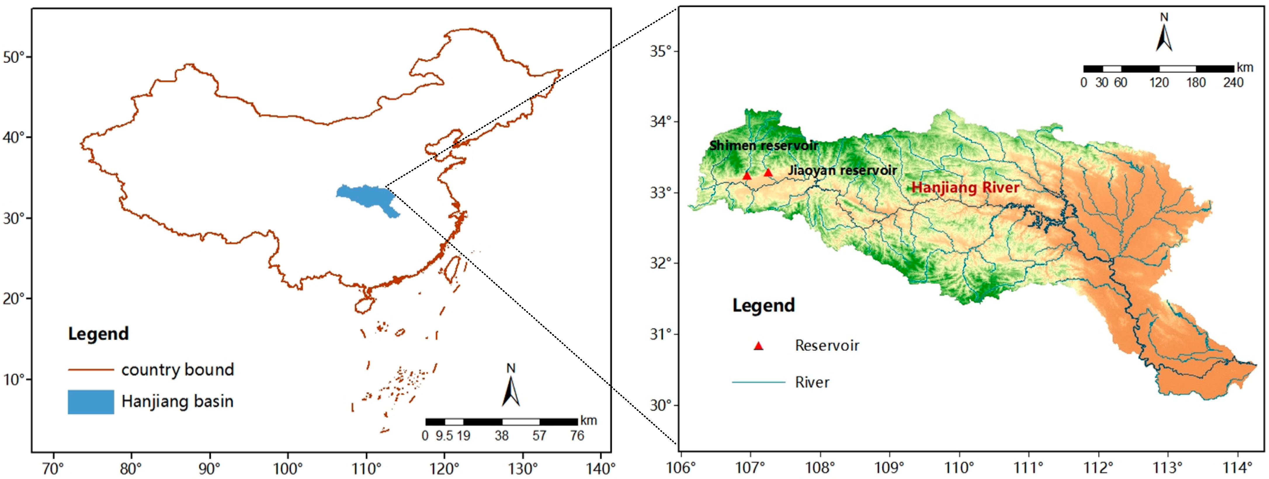
2. Study Area
2.1. Projects Overview
2.2. Problem Identification
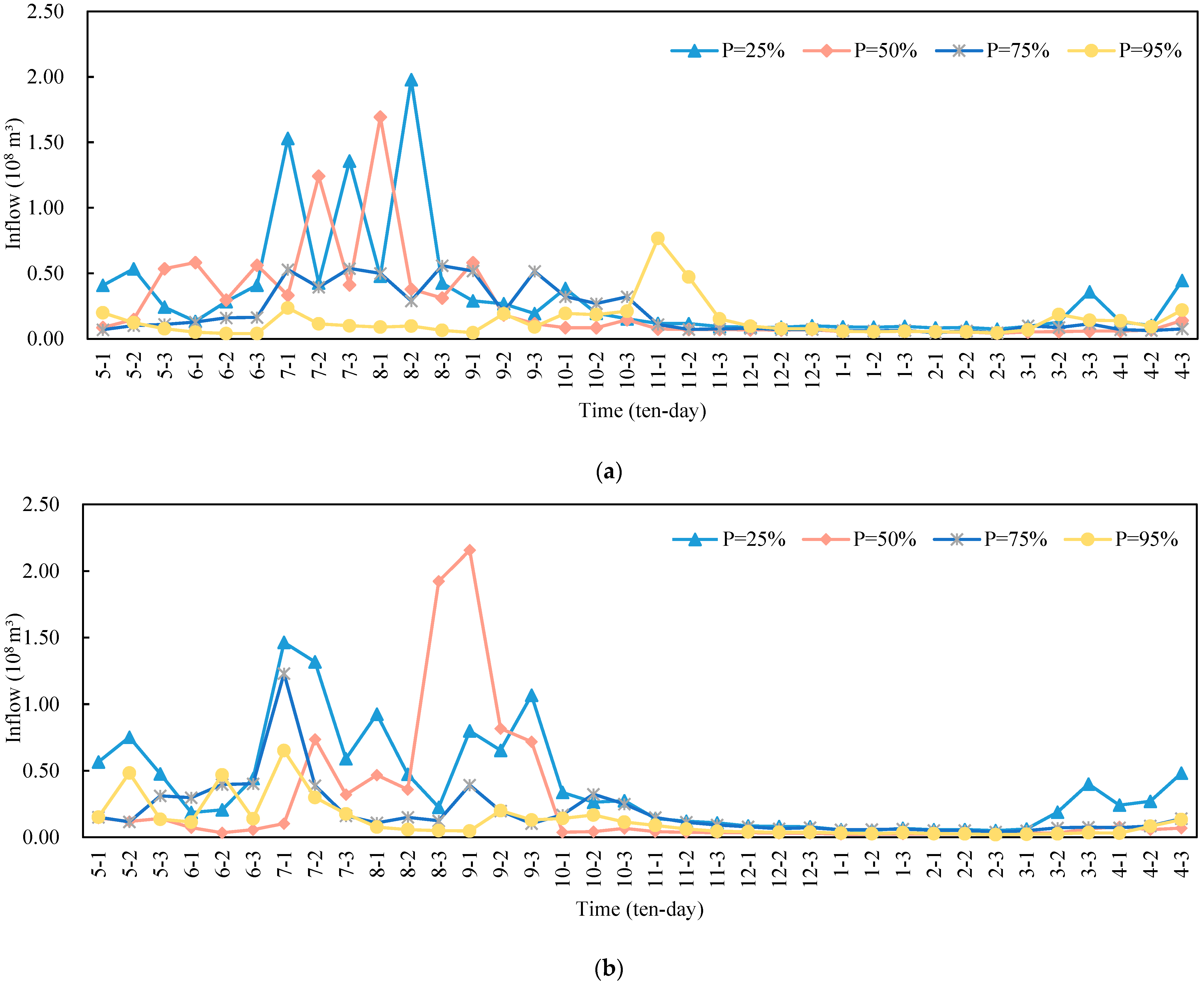
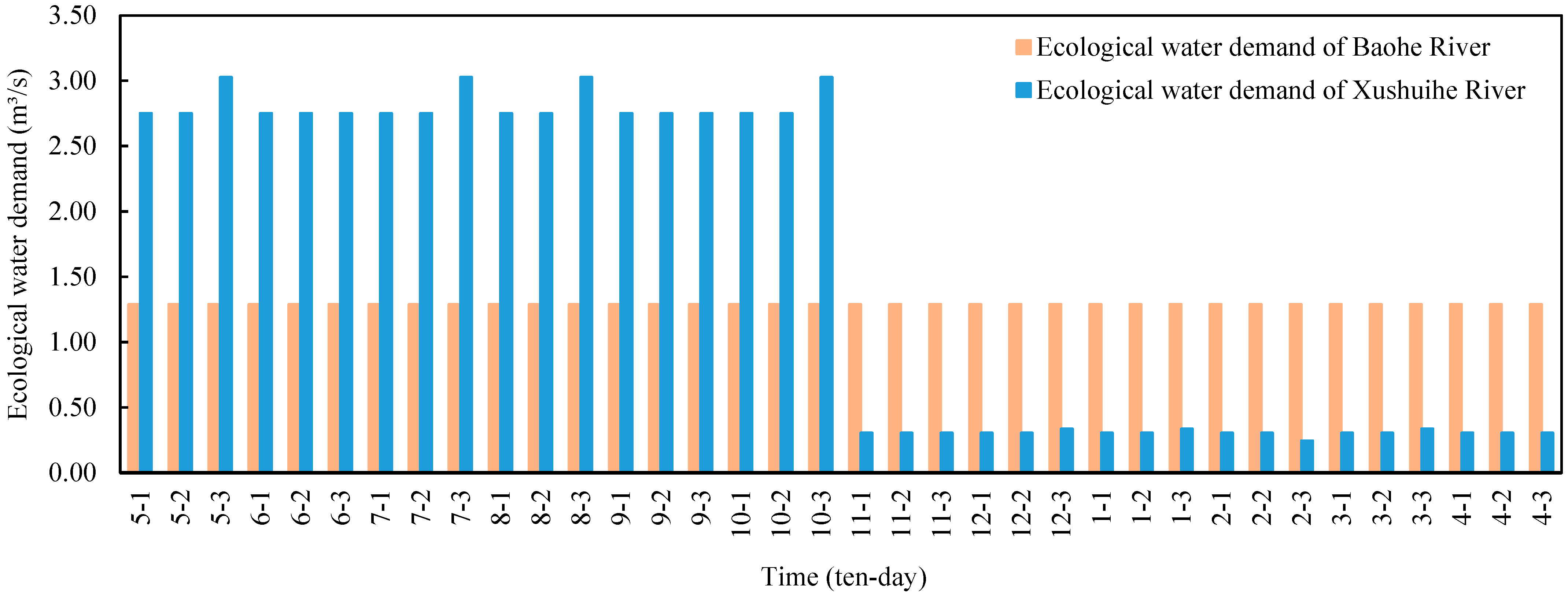
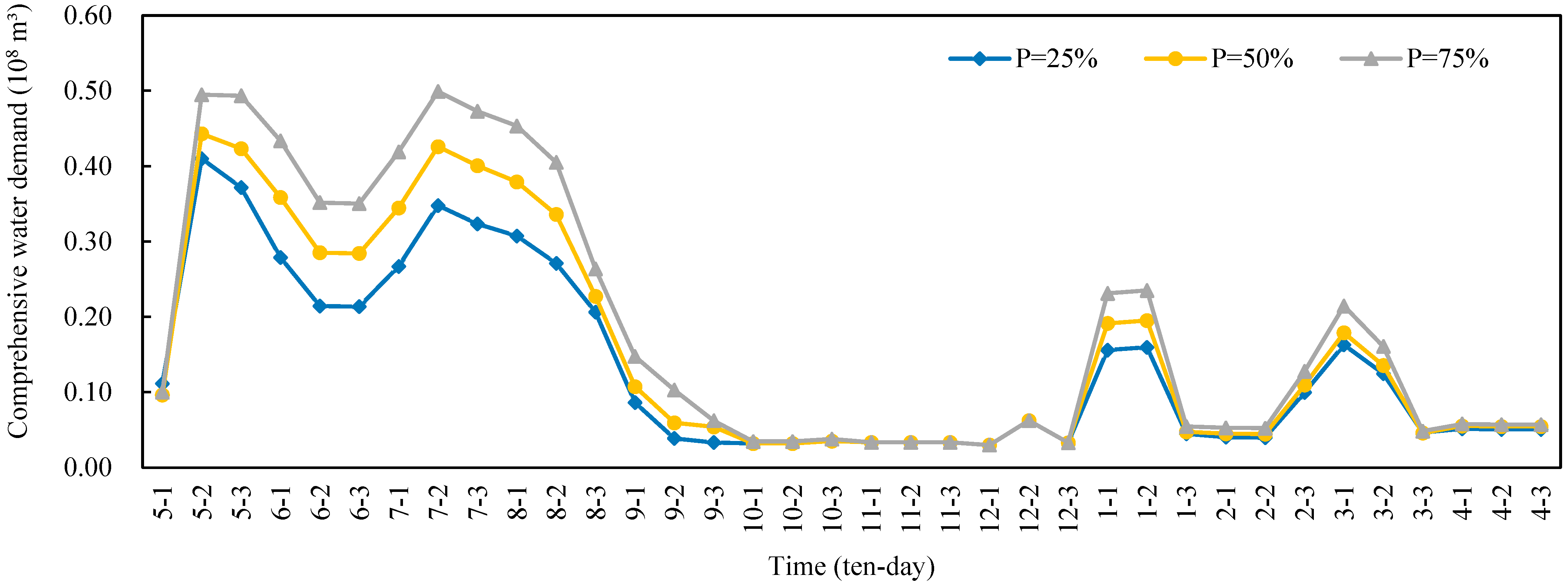
2.3. Typical Years Selection and Water Demand Analysis
3. Model Construction and Solving Algorithm
3.1. Model Construction
3.1.1. Objective Functions
- (1)
- Maximum comprehensive water supply.
- (2)
- Minimum ecological AAPFD value. The larger the ecological AAPFD value, the greater the influence of the reservoir on the downstream ecosystem, and vice versa.
3.1.2. Constraints
3.2. Solving Algorithm
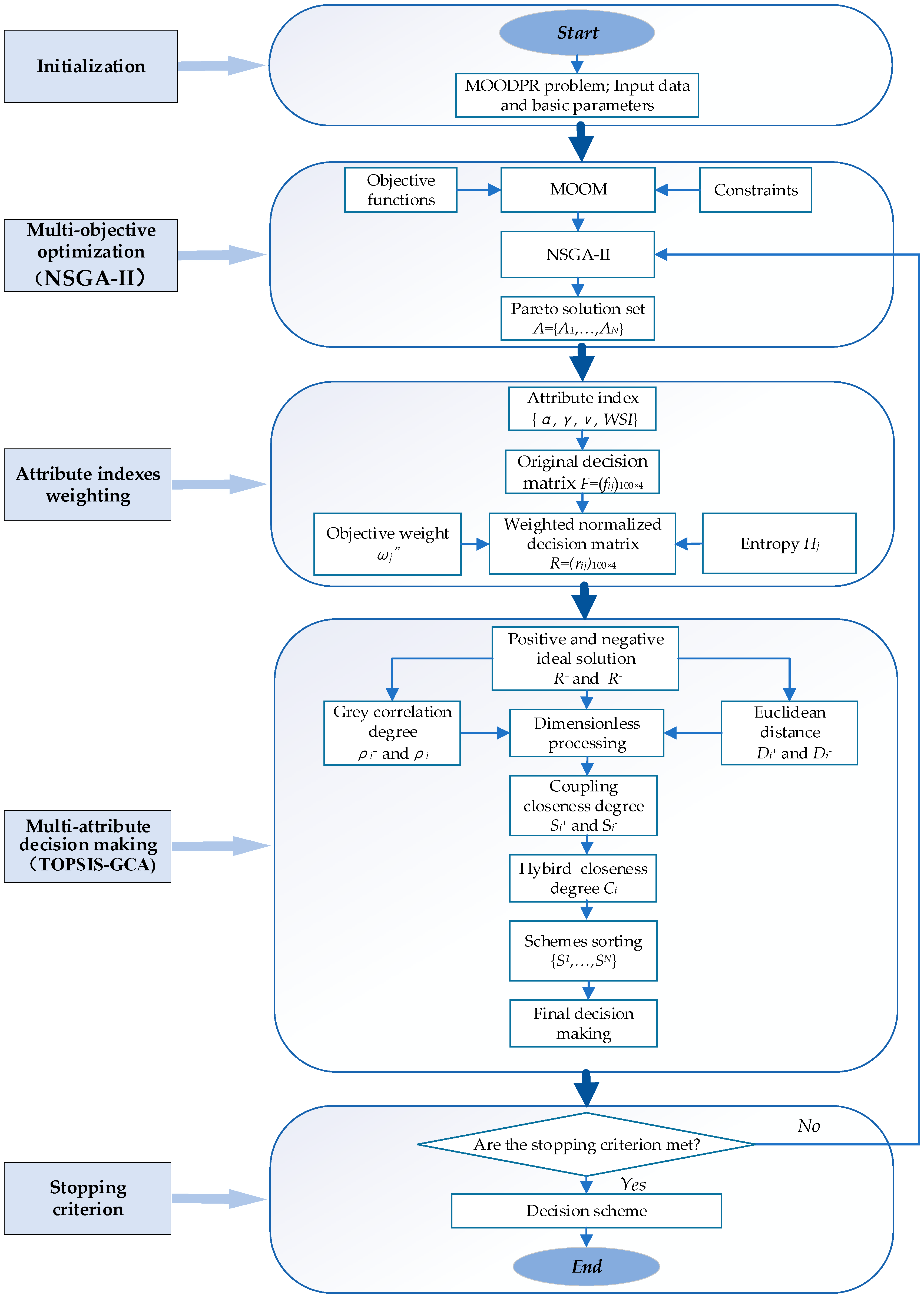
3.2.1. NSGA-II-TOPSIS-GCA
3.2.2. Application of NSGA-II-TOPSIS-GCA Algorithm for MOODPR Problem
| Algorithm 1: Detailed steps of NSGA-II-TOPSIS-GCA algorithm: |
| Input: The decision variables, objective functions, constraints, , , , , , and . |
| Output: and . |
| Step 1: Initialization |
| 1.1 = 100, = 1500, = 0.9, = 0.08, = 20, = 20, = 0. |
| 2 Initialization population randomly. |
| Step 2: Multi-objective optimization |
| 2.1 MOOM construction. |
| 2.2 Initialized population is non-dominated sorted, and individuals with better fitness are selected for genetic operation to generate the first-generation offspring population . |
| 2.3 Gen = 2, Merge offspring population and parent population. |
| 2.4 Individuals with better fitness are selected as the parent population. |
| 2.5 Perform genetic operation to obtain new offspring population. |
| 2.6 If , non-inferior solution set is obtained, otherwise , return to step 2.3. |
| Step 3: Attribute indexes weighting |
| 3.1 F Select attribute indexes , establish 4-dimensional original decision matrix. |
| 3.2 The 4-dimensional original decision matrix is normalized to obtain the 4-dimensional decision matrix. |
| 3.3 Calculate the entropy of attribute indexes: |
| 3.4 Calculate the objective weight of attribute indexes: |
| 3.5 Calculate the weighted normalized decision matrix , where . |
| Step 4: Multi-attribute decision making |
| 4.1 Determine the positive ideal solution and negative ideal solution of each scheme: |
| =, |
| = |
| 4.2 Calculate the grey correlation degree and of each scheme: |
| , where , , , |
| 4.3 Calculate Euclidean distance and of each scheme: |
| , |
| 4.4 Dimensionless processing for grey correlation degree and Euclidean distance determined in steps 4.2 and 4.3. |
| 4.5 Construct the coupling closeness degree and : |
| , |
| 4.6 Calculate hybrid closeness degree of each scheme: |
| 4.7 Sort all the schemes according to the hybrid closeness degree, and the scheme which has the largest hybrid closeness degree is taken as the final decision scheme. |
| Step 5: Stop |
| If the stop requirement is met, stop; otherwise return to Step 2. |
3.2.3. Attribute Indexes Selection
4. Results and Discussion
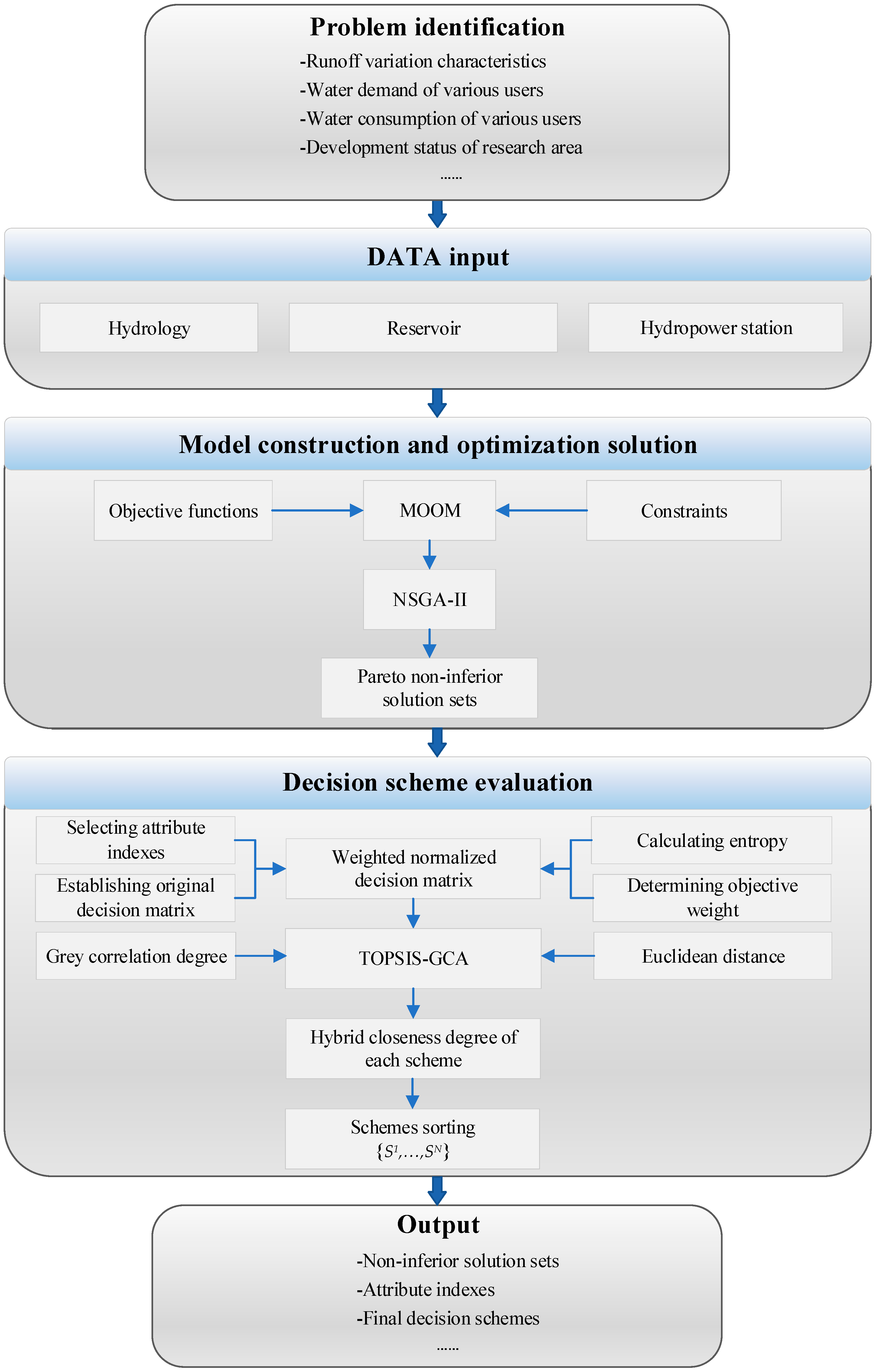
4.1. Model and Algorithm Application
- Problem identification. The relevant data of the research area are systematically collected, the development status of the research area is analyzed, and the existing problems are identified.
- Input parameters such as reservoirs and hydropower stations.
- Model construction. The MOOM is constructed according to the objective functions and constraints.
- Optimization solution. The non-inferior solution set is obtained.
- Scheme evaluation. The appropriate attribute indexes are selected and the 4-dimensional decision matrix is established. The TOPSIS-GCA is adopted to optimize the non-inferior solution set, so as to obtain the decision schemes.
- Output results, such as attribute indexes and decision schemes.
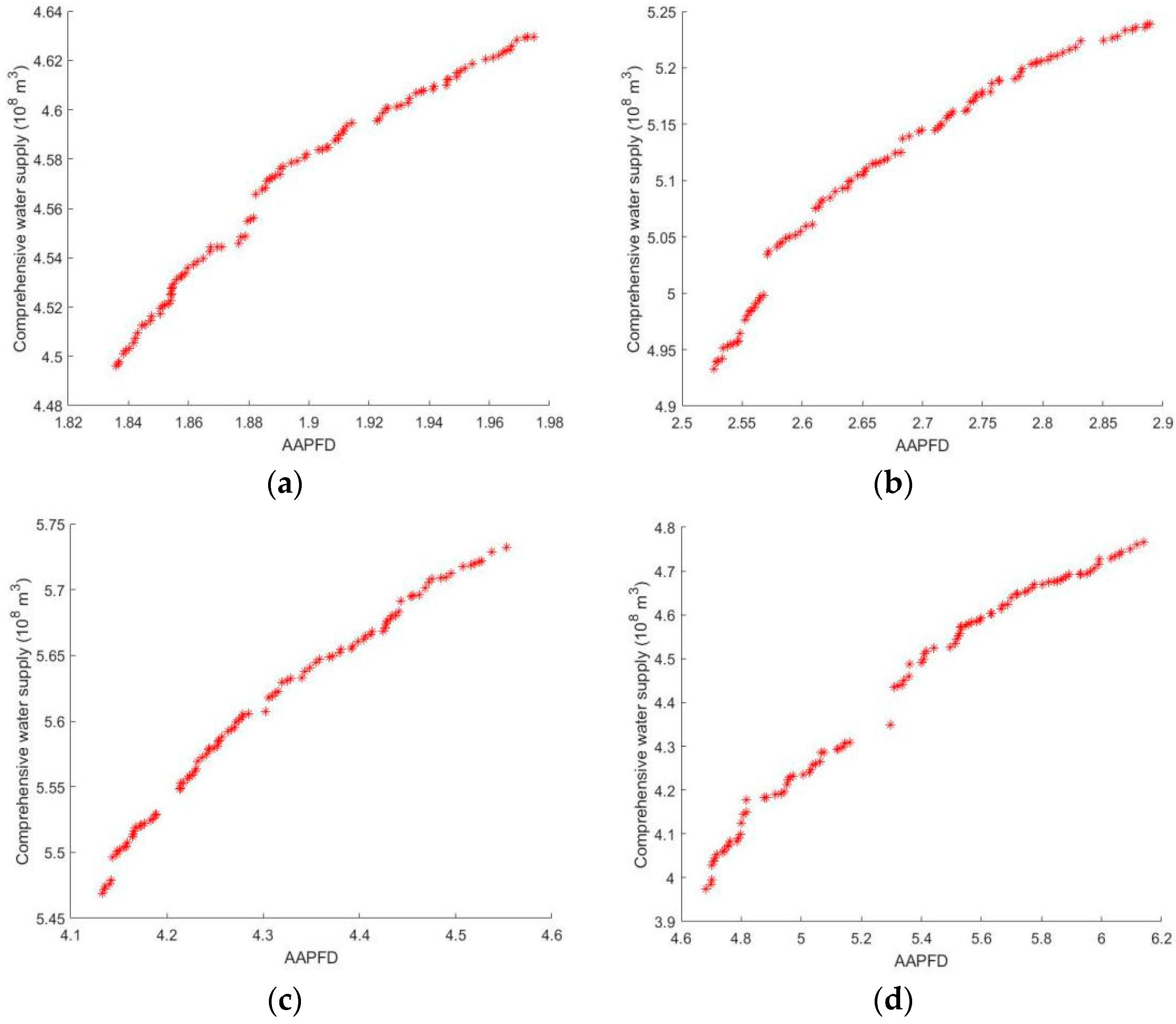
4.2. Pareto Solution Set
4.3. Decision Making Results
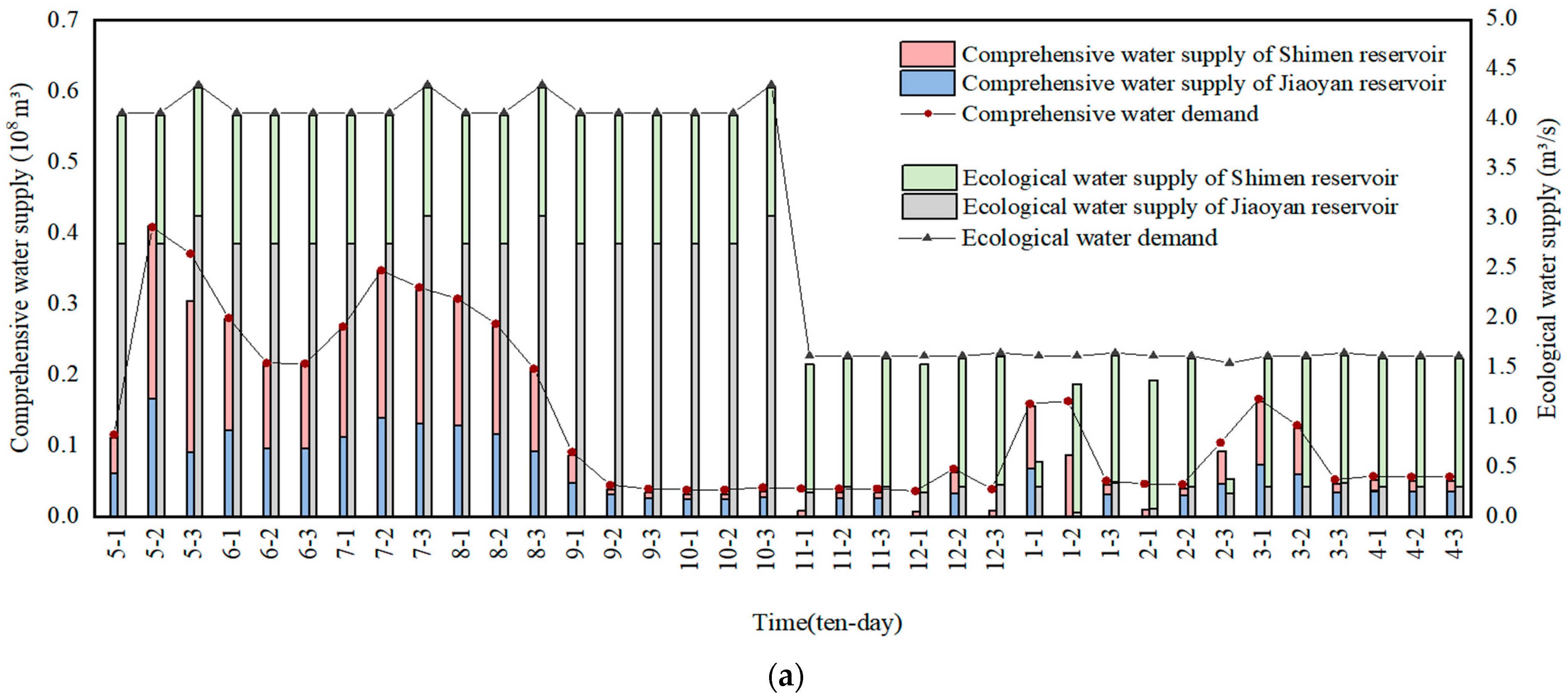
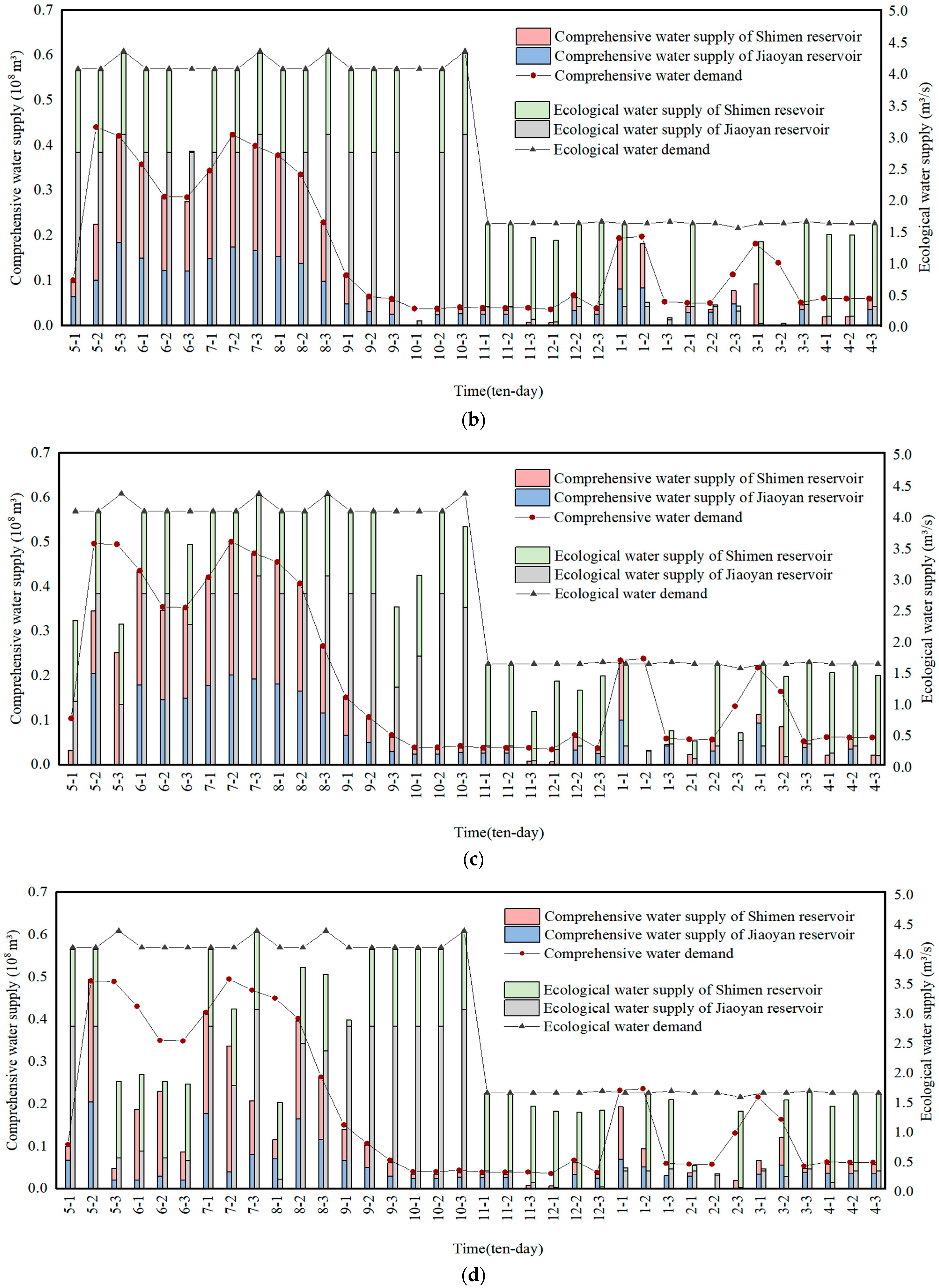
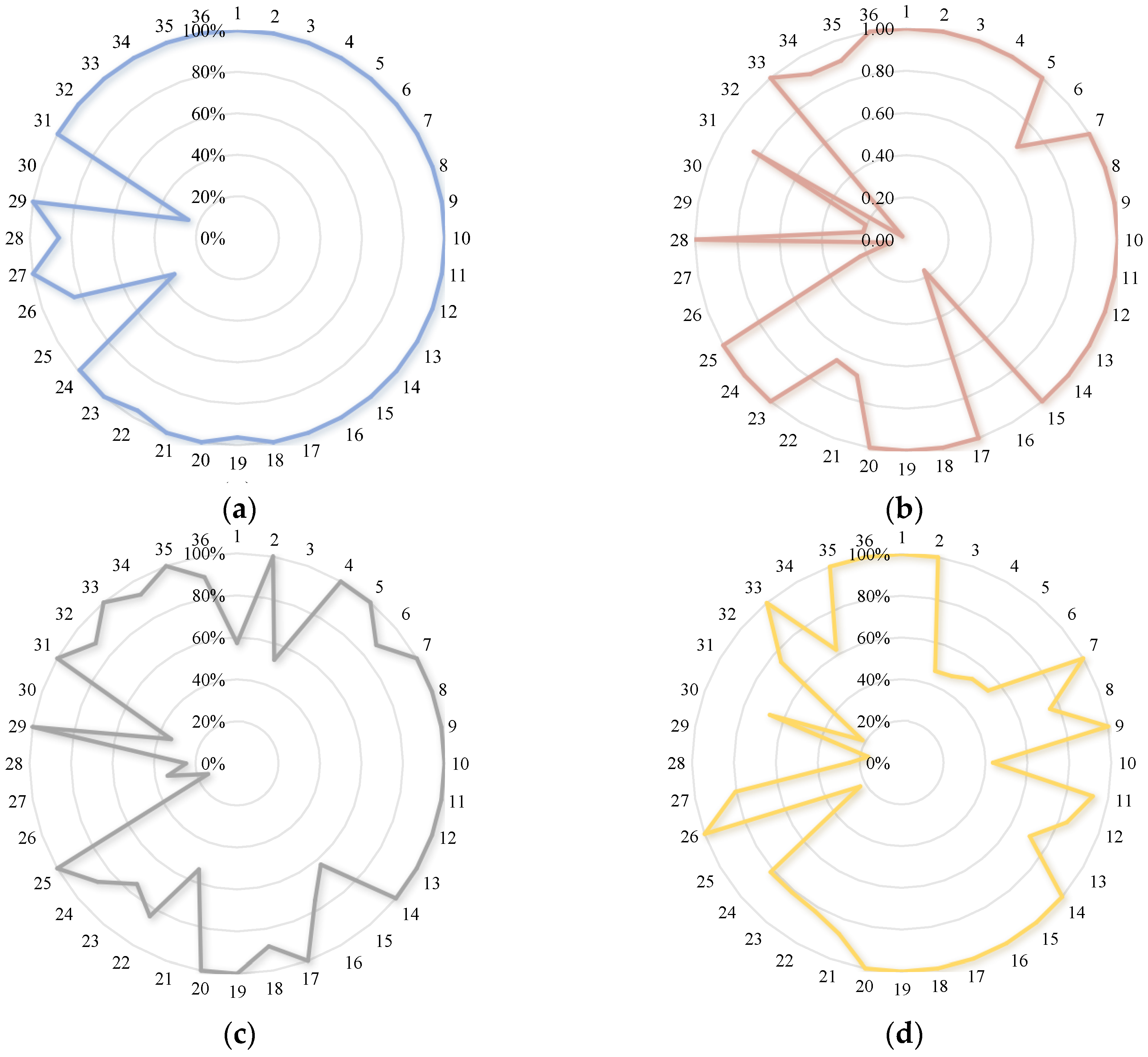
4.4. Decision Schemes Analysis
5. Conclusions
Author Contributions
Funding
Institutional Review Board Statement
Informed Consent Statement
Data Availability Statement
Acknowledgments
Conflicts of Interest
References
- Yan, D.F.; Xie, J.C.; Jiang, R.G. Trend and characteristics of runoff in upper reaches of Hanjiang River. J. Water Resour. Water Eng. 2016, 27, 13–19. [Google Scholar]
- Lu, Y.L.; Zhou, J.Z.; Wang, H. Multi-objective ecological optimal scheduling model of Three Gorges cascade hydro-junction and its solving method. Adv. Water Sci. 2011, 22, 780–788. [Google Scholar]
- Wang, X.B.; Chang, J.X.; Meng, X.J. Multi-objective scheduling of reservoirs in the lower Yellow River based on improved NSGA-II. J. Hydraul. Eng. 2017, 48, 135–145+156. [Google Scholar]
- Chen, Y.Y.; Mei, Y.D.; Cai, H. Study on Optimal Operation of Reservoirs in Ganjiang River Basin for Power Generation, Water Supply and Ecological Requirements. J. Hydraul. Eng. 2018, 49, 628–638. [Google Scholar]
- Jin, W.T.; Wang, Y.M.; Bai, T. Multi-objective scheduling and decision-making of Hanjiwei parallel reservoir in dry year. J. Hydroelectr. Power 2019, 38, 68–81. [Google Scholar]
- Reddy, J.M.; Kumar, N.D. Optimal Reservoir Operation Using Multi-Objective Evolutionary Algorithm. Water Resour. Manag. 2006, 20, 861–878. [Google Scholar] [CrossRef]
- Chang, L.C.; Chang, F.J. Multi-objective evolutionary algorithm for operating parallel reservoir system. J. Hydrol. 2009, 377, 12–20. [Google Scholar] [CrossRef]
- Afshar, M.H.; Azizipour, M.; Oghbaeea, B. Exploring the Efficiency of Harmony Search Algorithm for Hydropower Operation of Multi-reservoir Systems: A Hybrid Cellular Automat-Harmony Search Approach. Adv. Intell. Syst. Comput. 2017, 514, 252–260. [Google Scholar]
- Babel, M.S.; Gupta, A.D.; Nayak, D.K. A model for optimal allocation of water to competing demands. Water Resour. Manag. 2005, 19, 693–712. [Google Scholar] [CrossRef]
- Wang, S.N. Optimization analysis of water resources allocation in Northwest Henan based on MATLAB linear programming algorithm. Jilin Water Resour. 2021, 10, 22–27. [Google Scholar]
- Chen, C.; Kang, C.X.; Wang, J.W. Stochastic linear programming for reservoir operation with constraints on reliability and vulnerability. Water 2018, 10, 175. [Google Scholar] [CrossRef]
- Yue, W.C.; Yu, S.J.; Xu, M.; Rong, Q.Q.; Xu, C.; Su, M.R. A Copula-based interval linear programming model for water resources allocation under uncertainty. J. Environ. Manag. 2022, 317, 115318. [Google Scholar] [CrossRef] [PubMed]
- Bo, T.; Zhai, Q.; Guan, X. An MILP based formulation for short-term hydro generation scheduling with analysis of the linearization effects on solution feasibility. J. IEEE T. Power Syst. 2013, 28, 3588–3599. [Google Scholar]
- Yin, D.Q.; Li, X.; Wang, F.; Liu, Y.; Croke, B.F.W.; Jakeman, A.J. Water-energy-ecosystem nexus modeling using multi-objective, non-linear programming in a regulated river: Exploring tradeoffs among environmental flows, cascades small hydropower, and inter-basin water diversion projects. J. Environ. Manag. 2022, 308, 114582. [Google Scholar] [CrossRef] [PubMed]
- Hermida, G.; Castronuovo, E.D. On the hydropower short-term scheduling of large basins, considering nonlinear programming, stochastic inflows and heavy ecological restrictions. Int. J. Elec. Power 2018, 97, 408–417. [Google Scholar] [CrossRef]
- Ji, C.M.; Li, C.H.; Liu, X.Y. Dynamic programming algorithm based on functional analysis and its application in reservoir operation. J. Hydraul. Eng. 2016, 47, 1–9. [Google Scholar]
- Ai, X.S.; Guo, J.J.; Mu, Z.Y.; Chen, S.L.; Yang, B.Y.; Zhou, P.C. Multi-objective optimal scheduling model of cascade reservoirs and CPF-DPSA algorithm research. J. Hydraul. Eng. 2023, 54, 68–78. [Google Scholar]
- Saadat, M.; Asghari, K. Feasibility improved stochastic dynamic programming for optimization of reservoir operation. Water Resour. Manag. 2019, 33, 3485–3498. [Google Scholar] [CrossRef]
- Yves, M.; Gendreau, M.; Emiel, G. Benefit of PARMA modeling for long-term hydroelectric scheduling using stochastic dual dynamic programming. J. Water Resour. Plan. Manag. 2021, 147, 05021002. [Google Scholar]
- Rani, D.; Mourato, S.; Moreira, M. A Generalized Dynamic Programming Modelling Approach for Integrated Reservoir Operation. Water Resour. Manag. 2020, 34, 1335–1351. [Google Scholar] [CrossRef]
- Wu, X.Y.; Cheng, C.T.; Lund, J.R.; Niu, W.J.; Miao, S. Stochastic dynamic programming for hydropower reservoir operations with multiple local optima. J. Hydrol. 2018, 564, 712–722. [Google Scholar] [CrossRef]
- Chen, J.; Zhong, P.A.; Liu, W.; Wan, X.Y.; Yeh, W.G.A. Multi-objective risk management model for real-time flood control optimal operation of a parallel reservoir system. J. Hydrol. 2020, 590, 125264. [Google Scholar] [CrossRef]
- Seetharam, K.V. Three level rule curve for optimum operation of a multipurpose reservoir using genetic algorithms. Water Resour. Manag. 2021, 35, 353–368. [Google Scholar] [CrossRef]
- Liu, B.L.; Li, C.S.; Liu, F.Y. Multi-objective scheduling of cascade reservoirs in the upper reaches of the Yellow River based on NSGA-III. Yellow River 2022, 44, 140–144. [Google Scholar]
- Wang, Z.Z.; Wang, Y.T.; Chen, Y.W. Multi-objective reservoir regulation model based on simulation rules and intelligent optimization and its application. J. Hydraul. Eng. 2015, 43, 564–570+579. [Google Scholar]
- Liu, H.H.; Wang, N.; Xie, J.C.; Zhu, J.W.; Jiang, R.G.; Zhao, X. Application research on improved ant colony algorithm for optimal operation of reservoir group water supply. J. Hydroelectr. Power 2015, 34, 31–36. [Google Scholar]
- Moeini, R.; Afshar, M.H. Extension of the constrained ant colony optimization algorithms for the optimal operation of multi-reservoir systems. J. Hydroinform. 2013, 15, 155–173. [Google Scholar] [CrossRef]
- Safavi, R.H.; Enteshari, S. Conjunctive use of surface and ground water resources using the ant system optimization. Agric. Water Manag. 2016, 173, 23–34. [Google Scholar] [CrossRef]
- Xu, G.; Shu, Y.L.; Ren, Y.F.; Wu, B.Q. Real-time flood control operation model of Three Gorges Reservoir based on deep learning. J. Hydroelectr. Eng. 2022, 41, 60–69. [Google Scholar]
- Zhang, D.; Liu, J.Q.; Peng, Q.D.; Wang, D.S.; Yang, T.T.; Sorooshian, S.; Liu, X.F.; Zhuang, J.B. Modeling and simulating of reservoir operation using the artificial neural network, support vector regression, deep learning algorithm. J. Hydrol. 2018, 565, 720–736. [Google Scholar] [CrossRef]
- Qi, Y.T.; Bao, L.; Sun, Y.Y. A Memetic. Multi-objective Immune Algorithm for Reservoir Flood Control Operation. Water Resour. Manag. 2016, 30, 2957–2977. [Google Scholar] [CrossRef]
- Zou, Q.; Lu, J.; Zhou, C. Optimal operation of cascade reservoirs based on parallel hybrid differential evolution algorithm. J. Hydroelectr. Eng. 2017, 36, 57–68. [Google Scholar]
- Yin, X.L. Study on Water Supply-Power Generation-Ecological Optimal Operation of Reservoirs Based on Improved Multi-objective Whale Optimization Algorithm. Master’s Thesis, Huazhong University of Science and Technology, Wuhan, China, 2019. [Google Scholar]
- Li, J.; Wu, P.L. Multi-objective reservoir flood control operation scheme decision based on improved TOPSIS. Yellow River 2017, 39, 34–37. [Google Scholar]
- Liu, Y.A.; Wang, W.S. Set pair analysis and its application to optimization of standard schemes of urban flood control. J. North China Univ. Water Resour. Electr. Power Nat. Sci. Ed. 2018, 39, 77–80. [Google Scholar]
- Zhang, L.B.; Bai, Y.C.; Jin, J.L. Study on reservoir drought limit water level and water supply strategy optimization in irrigation district based on fuzzy set pair analysis. J. Hydraul. Eng. 2022, 53, 1154–1167. [Google Scholar]
- You, Z.Q.; Zou, Z.Q. Optimization of normal reservoir water level based on grey correlation ideal solution. Yangtze River 2017, 48, 101–104. [Google Scholar]
- Shen, X.; Fang, G.H.; Tan, Q.F.; Wen, X. Extraction of joint scheduling rules for wind-wind-water power generation system. Water Power 2019, 46, 114–117+126. [Google Scholar]
- Guo, Y.X.; Fang, G.H.; Wen, X.; Huang, X.F. Extraction method of scheduling rules for staggered generation of hydropower station. J. Hydroelectr. Eng. 2019, 38, 20–31. [Google Scholar]
- Ji, C.M.; Li, R.B.; Liu, D.; Zhang, Y.K.; Li, J.Q. Comprehensive evaluation of load adjustment plans for cascade hydropower stations based on moment estimation method and grey target model. Syst. Eng.–Theory Pract. 2018, 38, 1609–1617. [Google Scholar]
- Wang, L.P.; Yan, X.R.; Wang, B.Q.; Yu, H.J.; Ji, C.M. Interval number grey target decision-making model based on multi-dimensional association sampling and its application. Syst. Eng.–Theory Pract. 2019, 39, 1610–1622. [Google Scholar]
- Lu, Y.L.; Chen, J.S.; Qi, J.; Ji, P.; Zhou, J.Z. Research on reservoir multi-objective flood control operation decision-making method based on improved entropy weight and set pair analysis. Water Resour. Power. 2015, 33, 43–46. [Google Scholar]
- Ladson, A.R.; White, L.J. An Index of Stream Condition: Reference Manual, 2nd ed.; Department of Natural Resources and Environment: East Melbourne, Victoria, 1999; pp. 15–27. [Google Scholar]
- Du, Y. Risk Analysis and Multi-Attribute Risk Decision of Combined Flood Control Operation of Reservoirs. Ph.D. Thesis, Huazhong University of Science & Technology, Wuhan, China, 2018. [Google Scholar]
- Wei, N.; He, S.; Lu, K.; Xie, J.; Peng, Y. Multi-Stakeholder Coordinated Operation of Reservoir Considering Irrigation and Ecology. Water 2022, 14, 1970. [Google Scholar] [CrossRef]


| Parameter Category | Dead Water Level /m | Normal Water Level /m | Flood Control Level /m | Total Storage /108 m³ | Utilizable Capacity /108 m³ | Installed Capacity /MW | Maximum Flow through Water Turbine /(m³/s) | Minimum Flow through Water Turbine /(m³/s) |
|---|---|---|---|---|---|---|---|---|
| Jiaoyan reservoir | 540 | 585 | 585 | 2.125 | 1.718 | 50 | 87.5 | 0 |
| Shimen reservoir | 595 | 618 | 615 | 0.607 | 0.524 | 37.5 | 67.5 | 27 |
| Scheme Sets | Attribute Indexes | ||||
|---|---|---|---|---|---|
| α | γ | ν | WSI | ||
| A | Variation range | [0.750, 0.806] | [0.556, 0.857] | [0.743, 0.843] | [5.073, 11.603] |
| Standard deviation | 0.0249 | 0.133 | 0.0279 | 2.095 | |
| B | Variation range | [0.588, 0.689] | [0.494, 0.667] | [0.827, 0.892] | [21.826, 29.463] |
| Standard deviation | 0.0161 | 0.0486 | 0.0166 | 1.256 | |
| C | Variation range | [0.533, 0.639] | [0.400, 0.538] | [0.829, 0.990] | [23.758, 30.795] |
| Standard deviation | 0.0170 | 0.0509 | 0.0407 | 1.413 | |
| D | Variation range | [0.250, 0.528] | [0.111, 0.389] | [0.862, 0.995] | [37.566, 57.470] |
| Standard deviation | 0.0912 | 0.0594 | 0.0335 | 5.705 | |
| Scheme Sets | Positive Ideal Solutions | Negative Ideal Solutions |
|---|---|---|
| A | R+ = (0.0262, 0.0326, 0.0233, 0.0157) | R− = (0.0243, 0.0211, 0.0265, 0.0358) |
| B | R+ = (0.0272, 0.0294, 0.0240, 0.0210) | R− = (0.0225, 0.0218, 0.0259, 0.0282) |
| C | R+ = (0.0264, 0.0285, 0.0227, 0.0215) | R− = (0.0241, 0.0212, 0.0273, 0.0279) |
| D | R+ = (0.0320, 0.0378, 0.0222, 0.0192) | R− = (0.0152, 0.0108, 0.0276, 0.0294) |
| Scheme No. | A | B | C | D | ||||
| Hybrid Closeness Degree | Scheme Sort | Hybrid Closeness Degree | Scheme Sort | Hybrid Closeness Degree | Scheme Sort | Hybrid Closeness Degree | Scheme Sort | |
| 1 | 0.6919 | 71 | 0.5632 | 99 | 0.5243 | 35 | 0.6796 | 31 |
| 2 | 0.6802 | 14 | 0.5563 | 94 | 0.5231 | 36 | 0.6794 | 97 |
| 3 | 0.6715 | 44 | 0.5538 | 95 | 0.5230 | 37 | 0.6751 | 1 |
| 4 | 0.6706 | 18 | 0.5481 | 80 | 0.5229 | 1 | 0.6699 | 95 |
| 5 | 0.6681 | 30 | 0.5476 | 81 | 0.5216 | 38 | 0.6599 | 14 |
| 6 | 0.6664 | 84 | 0.5467 | 100 | 0.5198 | 39 | 0.6589 | 54 |
| 7 | 0.6660 | 74 | 0.5462 | 96 | 0.5175 | 40 | 0.6589 | 61 |
| 8 | 0.6644 | 37 | 0.5461 | 82 | 0.5155 | 92 | 0.6587 | 43 |
| 9 | 0.6591 | 98 | 0.5435 | 83 | 0.5144 | 41 | 0.6559 | 87 |
| 10 | 0.6524 | 79 | 0.5419 | 84 | 0.5140 | 42 | 0.6552 | 75 |
| 11 | 0.6520 | 59 | 0.5408 | 7 | 0.5117 | 43 | 0.6272 | 71 |
| 12 | 0.6519 | 3 | 0.5404 | 97 | 0.5094 | 93 | 0.6248 | 93 |
| 13 | 0.6483 | 28 | 0.5390 | 8 | 0.5089 | 44 | 0.6230 | 70 |
| ··· | ··· | ··· | ··· | ··· | ··· | ··· | ··· | ··· |
| 99 | 0.3270 | 65 | 0.4657 | 64 | 0.3746 | 33 | 0.3139 | 52 |
| 100 | 0.3094 | 1 | 0.4647 | 1 | 0.3717 | 34 | 0.2878 | 55 |
| Scheme Sets | Decision Scheme No. | α | γ | ν | WSI |
|---|---|---|---|---|---|
| A | 71 | 0.806 | 0.857 | 0.748 | 5.073 |
| B | 99 | 0.611 | 0.663 | 0.880 | 20.963 |
| C | 0.556 | 0.429 | 0.938 | 30.610 | |
| D | 31 | 0.498 | 0.305 | 0.987 | 40.024 |
| Scheme Sets | Objectives | Water Demand | Water Supply | Guarantee Rate | Water Shortage | Water Shortage Depth | Number of Maximum Continuous Water Shortage Periods | |
|---|---|---|---|---|---|---|---|---|
| Flood Season | Non-Flood Season | |||||||
| /108 m³ | /108 m³ | /% | /% | /108 m³ | /% | |||
| A | Comprehensive water supply | 4.828 | 4.577 | 94% | 63% | 0.251 | 5 | 1 |
| Ecology water supply | 0.931 | 0.906 (1.891) 1 | 100% | 61% | 0.025 | 3 | 2 | |
| B | Comprehensive water supply | 5.702 | 4.996 | 89% | 39% | 0.706 | 12 | 3 |
| Ecology water supply | 0.931 | 0.813 (2.565) 1 | 89% | 44% | 0.118 | 13 | 4 | |
| C | Comprehensive water supply | 6.726 | 5.563 | 78% | 44% | 1.163 | 17 | 3 |
| Ecology water supply | 0.931 | 0.804 (4.230) 1 | 67% | 39% | 0.127 | 14 | 4 | |
| D | Comprehensive water supply | 6.726 | 4.212 | 61% | 39% | 2.514 | 37 | 4 |
| Ecology water supply | 0.931 | 0.735 (4.953) 1 | 50% | 33% | 0.196 | 21 | 6 | |
Disclaimer/Publisher’s Note: The statements, opinions and data contained in all publications are solely those of the individual author(s) and contributor(s) and not of MDPI and/or the editor(s). MDPI and/or the editor(s) disclaim responsibility for any injury to people or property resulting from any ideas, methods, instructions or products referred to in the content. |
© 2024 by the authors. Licensee MDPI, Basel, Switzerland. This article is an open access article distributed under the terms and conditions of the Creative Commons Attribution (CC BY) license (https://creativecommons.org/licenses/by/4.0/).
Share and Cite
Wei, N.; Peng, Y.; Lu, K.; Zhou, G.; Guo, X.; Niu, M. Multi-Objective Optimal Operation Decision for Parallel Reservoirs Based on NSGA-II-TOPSIS-GCA Algorithm: A Case Study in the Upper Reach of Hanjiang River. Appl. Sci. 2024, 14, 3138. https://doi.org/10.3390/app14083138
Wei N, Peng Y, Lu K, Zhou G, Guo X, Niu M. Multi-Objective Optimal Operation Decision for Parallel Reservoirs Based on NSGA-II-TOPSIS-GCA Algorithm: A Case Study in the Upper Reach of Hanjiang River. Applied Sciences. 2024; 14(8):3138. https://doi.org/10.3390/app14083138
Chicago/Turabian StyleWei, Na, Yuxin Peng, Kunming Lu, Guixing Zhou, Xingtao Guo, and Minghui Niu. 2024. "Multi-Objective Optimal Operation Decision for Parallel Reservoirs Based on NSGA-II-TOPSIS-GCA Algorithm: A Case Study in the Upper Reach of Hanjiang River" Applied Sciences 14, no. 8: 3138. https://doi.org/10.3390/app14083138