Optical Design and Stray Light Analysis of Underwater Spectral Radiometer

Abstract

Underwater spectral detection plays an important role in the study of the underwater environment, ecology, oceanography, and environmental monitoring. A kind of underwater spectral radiometer that can observe the distribution of underwater spectral radiation bidirectionally has been developed. The flat-field concave holographic grating is used as the only optical component, the optical design parameters are optimized, and the system is miniaturized. The mechanism of stray light generation in the spectrometer is studied, and a method of suppressing stray light is proposed and simulated. The level of stray light in the system is suppressed to the order of 10⁻⁴, the signal-to-noise ratio of the system is improved, and the ability to detect weak light is enhanced. The wavelength calibration experiment was completed, and the experimental results show that the wavelength resolution of the underwater spectral radiometer is better than 3 nm. Finally, the quantitative relationship between spectral irradiance and digital output is obtained through radiation in the calibration of the system.

1. Introduction

The ocean is the origin of life on Earth. About 71% of the Earth’s surface is covered by water, and the ocean, as the largest part, harbors rich natural resources, especially fisheries resources. For a long time, obtaining food from the ocean and lakes has been one of the crucial means of sustenance for humanity. Since the 20th century, human activities and global climate change have led to ecological degradation in the water bodies of many countries. Inland and nearshore marine water quality has generally declined, with a substantial reduction in the distribution area of seagrass beds and coral reefs. Additionally, the widespread issue of algal blooms is showing a global trend. Aquatic economic species are experiencing a decrease in age and size, and there is a noticeable trend of desertification on the seabed [1]. Water plants and large algae, similar to terrestrial plants, play the role of primary producers of water. Through photosynthesis, they contribute 50% of the Earth’s fixed carbon, playing a crucial role in the global carbon cycle. Light serves as the primary energy source for aquatic ecosystems, influencing the photosynthesis of phytoplankton and, consequently, algal content and primary productivity [2,3]. To protect water resources, improve water quality, and ensure the healthy development of aquatic ecosystems, it is essential to focus on and maintain the lighting conditions in the water. Underwater spectral measurements are of significant importance for monitoring water quality, the health of ecosystems, and changes in marine and freshwater environments.

Water optical property measurement techniques are the driving force behind the development of marine optics [4]. In the mid-19th century, as attention to the quality of water and environmental conditions increased, scientists began seeking a convenient method to measure the transparency of water. Consequently, the transparency disk emerged, becoming a portable and easy-to-use tool for monitoring water quality in field environments. In the 1930s, the advent of photomultiplier tubes brought about a significant revolution in the development of underwater optical technology, providing valuable experiential foundations for understanding the interaction between light and seawater. In the 1980s, the development of water color satellite remote sensing technology sparked widespread interest in the optical properties of the oceans. The progress in ocean optical measurement techniques has propelled research and development in marine ecosystems, marine environmental conservation, carbon cycling, and global climate change [5]. The variation and distribution of marine water color are influenced by substances in the upper water layer. To gain a thorough understanding of the optical properties of seawater and their impact on light transmission, it is necessary to employ high-performance optical measuring instruments for water color remote sensing research. However, marine water color remote sensing instruments, primarily relying on remote sensing, are subject to interference from atmospheric Rayleigh scattering, aerosol scattering, and other factors. This leads to disparities between the apparent optical parameters of water bodies observed by satellites and the actual apparent optical parameters of the water. Additionally, due to factors such as cloud cover and low light, optical remote sensing is unable to observe high-dynamic water bodies for a significant portion of the time. In contrast, in-situ measurements, as a method for water monitoring, can overcome these challenges [6]. The in-orbit data from satellite water color remote sensing instruments needs to be verified with on-site measurement data that possesses sufficient accuracy, repeatability, and traceability [7]. There are three methods for on-site observation in water color remote sensing: above-water method, skylight obstruction method, and underwater profile method. Among them, the underwater profile method is widely recognized as a more accurate measurement technique, commonly used for measuring the apparent optical properties of water bodies, particularly in large oceanic areas. The underwater light field profile distribution holds significant importance in the study of marine physical and biological processes, such as marine primary productivity, upper-layer heat balance, remote sensing inversion of water color elements, and interactions in marine biogeochemical processes [8].

Long-term, large spatial-scale aquatic environmental monitoring plays an important role in human understanding and comprehension of the oceans [9]. In order to realize global water ecological monitoring, it is extremely necessary to develop high-sensitivity, high-precision, stable, and reliable field sensors. Currently, representative in situ ocean radiometers internationally typically possess a spectral resolution of generally 10 nm or higher. However, with advancements in ocean color remote sensing technology, high-spectral and high-resolution instruments are continuously being developed. Examples include the Ocean Color Instrument (OCI) on the U.S. PACE satellite (focused on phytoplankton, aerosols, clouds, and the marine ecosystem), the Hyperspectral Imager for Coastal Ocean (HICO) utilized for coastal ocean remote sensing on the International Space Station, and the Advanced Hyperspectral Imager (AHSI) with full spectral resolution on China’s Gaofen-5 satellite, all with spectral resolutions at 5 nm. A resolution of 10 nm is no longer sufficient for the latest generation of water color remote sensing instruments. Therefore, based on the consideration of the demand for spectral radiance observation of water bodies, this paper designs a miniature underwater spectral radiometer suitable for underwater profiling. The instrument uses concave holographic grating as a spectral component, and the spectral observation range is 400–950 nm, covering the spectral bandwidth requirements of all bands of underwater spectral observation and water color sensors. The full-band spectral resolution is better than 3 nm, which has the advantages of a broad spectrum, high resolution, and small size. In addition, the stray light in the optical structure of the spectral radiometer is simulated and analyzed. The measures to suppress the stray light are proposed, and the effect of inhibiting the stray light is analyzed. Laboratory calibration was carried out for the principle prototype, and the wavelength calibration results showed that the spectral resolution of the instrument met the design requirements. The radiation calibration experiment was completed and the spectral irradiance response curve of the instrument was obtained.

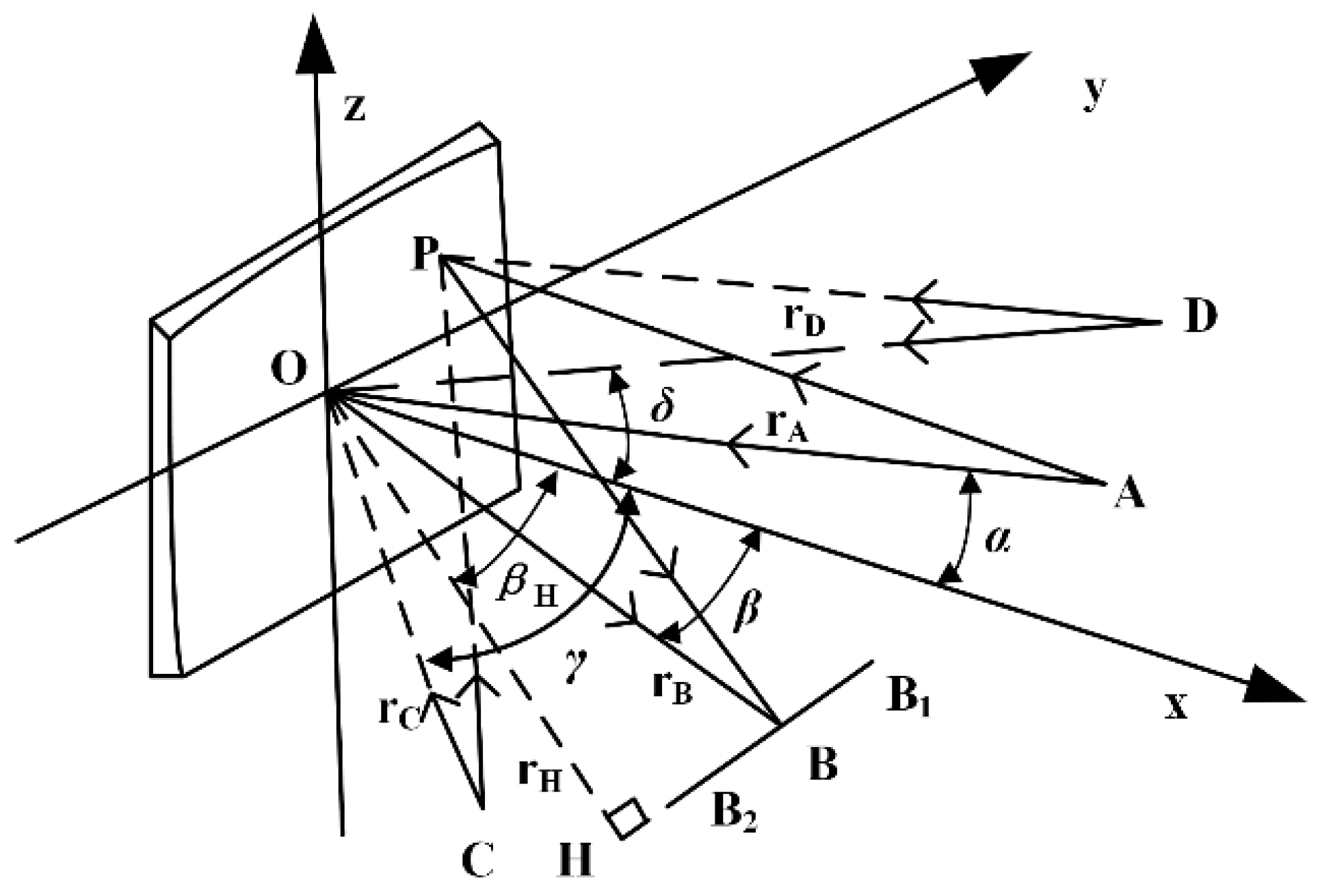
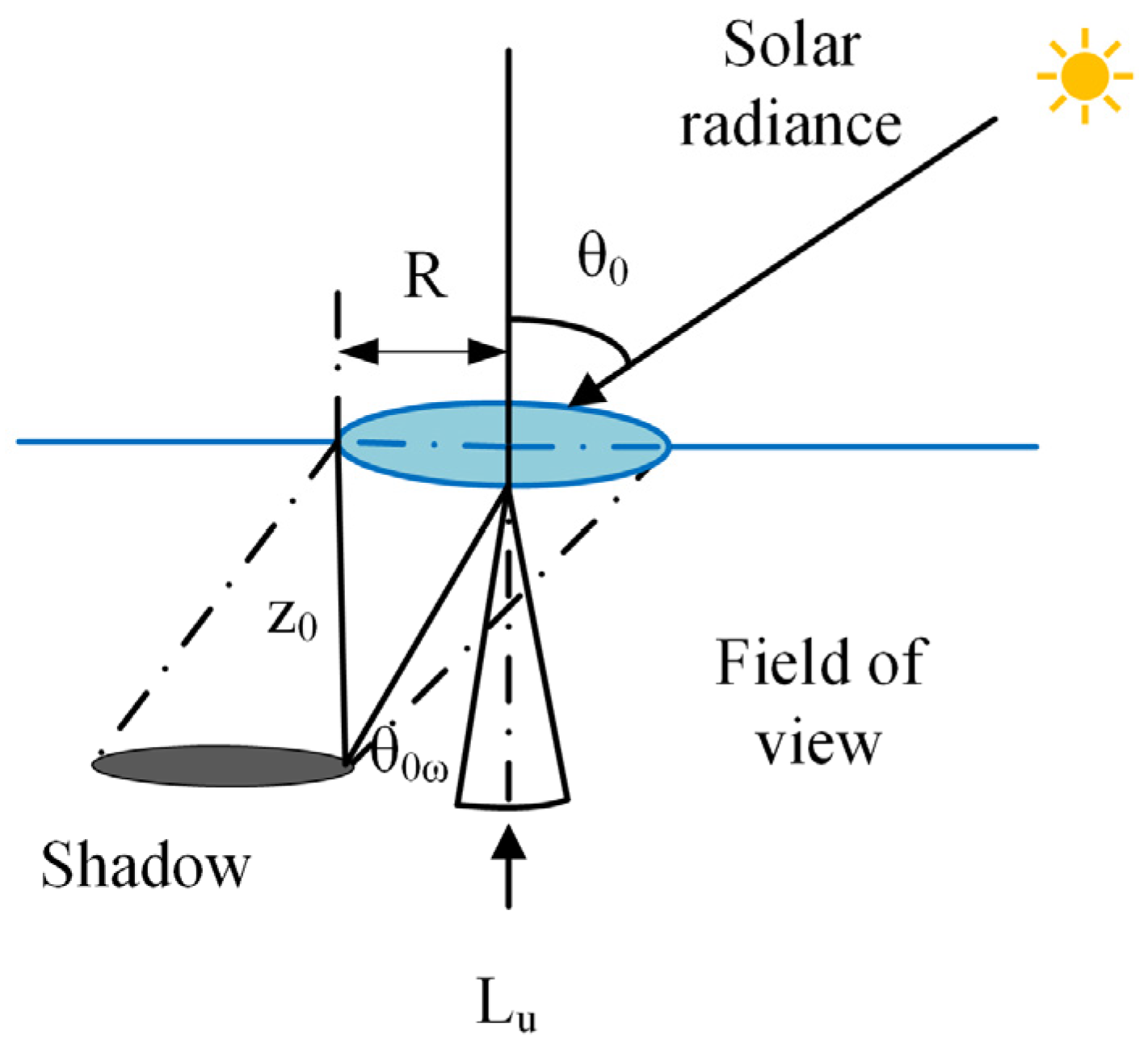
2. Theoretical Foundation

The spectral measurement of upward and downward irradiance and radiance in the ocean at different depths provides one of the best methods for studying the optical characteristics of seawater [10]. Compared to the measurement of spectral radiance on land, there are numerous factors that affect underwater radiance measurements. In the field measurements of water color remote sensing, the key challenges to address include a wide dynamic range, self-shadowing effects, and the signal-to-noise ratio issue [11].

The light entering the water is primarily composed of two parts: direct radiation from the sun and diffuse radiation from the sky. As sunlight passes through the sea surface and enters the seawater, the light undergoes attenuation due to the absorption and scattering within the water. According to the Beer–Lambert Law, light experiences exponential decay as it propagates through water. Taking the downwelling spectral irradiance in the water as an example, let us analyze the irradiance conditions observed by the underwater spectral radiometer. Assuming the water in the ocean is homogeneous, the downward spectral irradiance located z meters below the sea surface can be represented by Equation (1).

$$E_d(\lambda ,z)=E_d(\lambda ,0^{-})e^{-K_d(\lambda )z}$$

(1)

In Equation (1), $E_d(\lambda ,z)$ and $E_d(\lambda ,0^{-})$, respectively, represent the downward spectral irradiance at a depth of z meters below the sea surface and 0 m below the sea surface. $K_d(\lambda )$ represents the attenuation coefficient of the water for a wavelength $\lambda$. From Equation (1), it is evident that after passing through a certain depth of seawater, spectral radiation attenuation is quite pronounced. In order to measure underwater profile data at a specific depth, an underwater spectroradiometer should possess the capability of detecting faint oceanic light.

In addition, the underwater light field distribution is determined by the inherent optical properties of the water. The presence of underwater optical instruments can interfere with the light field distribution around the instrument, and this effect is known as the instrument’s self-shadowing effect. Self-shadowing refers to the shadow impact caused by the external structure of the sensor itself, and underwater optical instruments are generally affected by the self-shadowing effect [12]. Taking the measurement of upward spectral radiance as an example to analyze the impact of the instrument’s self-shadowing effect on the measurement results, the shadow situation generated during underwater upward spectral radiance measurement is illustrated in Figure 1.

An underwater spectral radiometer is typically designed in a cylindrical structure, represented by the disk in Figure 1, which symbolizes the instrument’s housing. When sunlight is incident at a specific solar zenith angle, a shadow is cast on the opposite side of the instrument [13]. When an underwater spectral radiometer measures the upward radiance spectrum $L_u(\lambda )$ in the water, the instrument’s field of view experiences a reduction in spectral energy due to self-shadowing. Therefore, the presence of shadows within the instrument’s field of view inevitably leads to a discrepancy between the measured values and the actual values. The measurement error in the upward spectral irradiance $E_d(\lambda )$ in the water, influenced by the instrument’s characteristics, follows mechanisms similar to those described for the measurement of upward radiance $L_u(\lambda )$. The key difference is that the solid angle for the observation field of upward spectral irradiance is 2π. Consequently, the measurement error caused by shadowing effects in upward spectral irradiance is much smaller than the radiance measurement error [14].

As shown in Figure 1, when the instrument is absent, the upward spectral radiance at point $z_0$ is related to the upward spectral radiance at point 0 on the water surface as follows:

$$L_u^{true}(z_0)=L_u^{true}(0)exp(-K_u{z}_0)$$

(2)

where $K_u$ is the attenuation coefficient of the water body, which mainly depends on the absorption and scattering of the water body. Since the scattering coefficient of the water body is much smaller than the absorption coefficient of the water body, only the influence of the absorption coefficient $a$ on the attenuation of the water body is considered. When the instrument exists, there is no ascending spectral radiance at the water surface due to the occlusion of the instrument, and what the instrument observes is the value of the ascending radiance underwater $z_0$ propagating to the water surface 0:

$$\begin{array}{c}{L}_u^{measure}(0)=L_u^{true}(0)exp(-K_u{z}_0)exp(-a{z}_0) \\ \approx L_u^{true}(0)exp(-2a{z}_0)\end{array}$$

(3)

The relationship between $z_0$ and the underwater refraction Angle ${\theta }_{o\omega }$ of the zenith Angle of the sun and the instrument radius R is as follows:

$$z_0=\frac{R}{\tan ({\theta }_{o\omega })}$$

(4)

The measurement error percentage caused by the self-shadowing effect of the instrument is denoted by $\epsilon$, which represents the difference between the actual value and the true value divided by the true value.

$$\epsilon =\frac{L_u^{true}-L_u^{measure}}{L_u^{true}}$$

(5)

The expression of self-shading error is obtained by simultaneous Equations (2)–(5):

$$\epsilon =1-exp(-\frac{2aR}{\tan {\theta }_{o\omega }})$$

(6)

According to Formula (6), the measurement error caused by the self-shadow effect of the instrument is related to the water absorption coefficient $a$, the outer radius of the sensor R, and the refraction angle ${\theta }_{o\omega }$ of the solar zenith angle [15]. In order to ensure the final measurement accuracy of the instrument, efforts should be made to minimize the measurement error caused by the instrument’s self-shadowing effects. Strictly controlling the overall dimensions of the instrument is crucial for meeting the design requirements of miniaturization and broad spectral coverage.

3. Underwater Spectral Radiometer Design

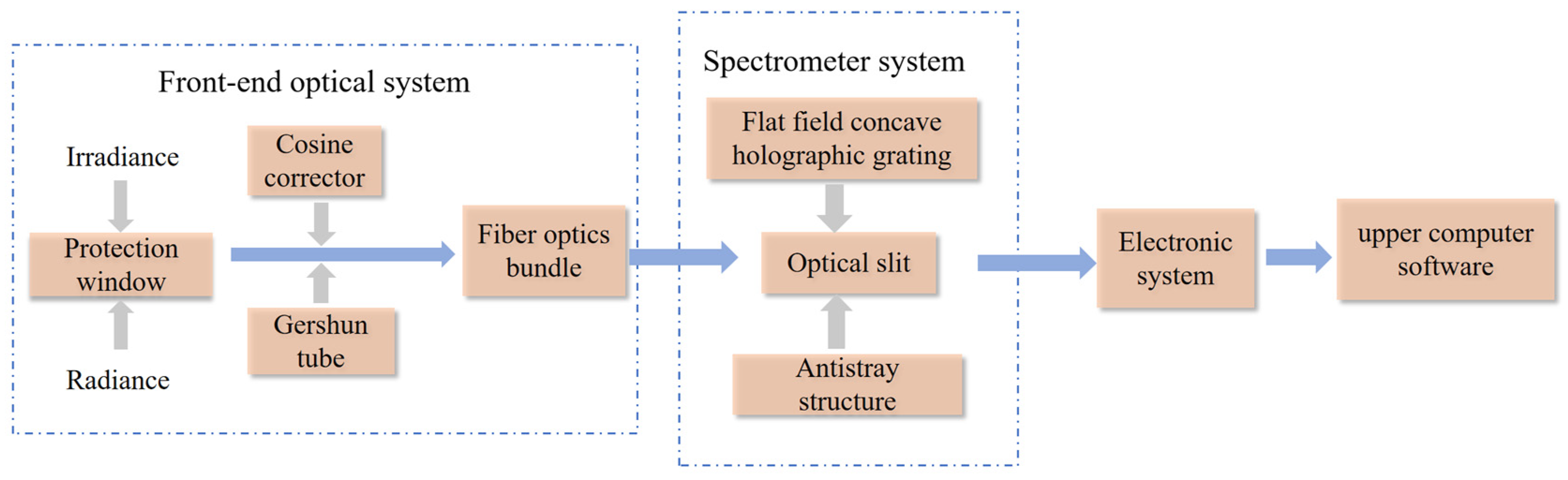
3.1. Overall Design

The hardware design of the underwater spectral radiometer consists of four main components, as illustrated in Figure 2. These components include the front-end optical system, spectrometer system, electronic system, and upper-level software. Except for the upper-level software, all other parts are integrated into the instrument’s mechanically sealed structure. The optical module serves as the core unit of the underwater spectral radiometer and is the focus of this study.

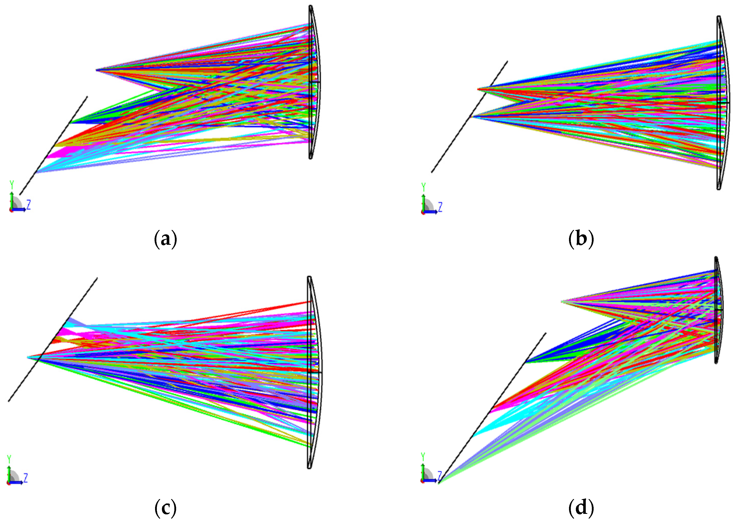
3.2. Front-End Optical System

When a spectral radiometer is used to observe the bidirectional distribution of spectral radiation in the water body, different front-end optical systems need to be selected because of different observation targets. When observing the spectral radiance of the water body, the field of view of the radiance sensor is 2–18° according to the Marine optical specifications. In this paper, a Gershun tube (Diaphragm cylinder structure) is selected to limit the observation field of the instrument. The Gershun tube is a field-of-view regulating device that can be connected by optical fiber. In order to minimize the influence of stray light and eliminate the radiation from the light source outside the field of view, a stray light-blocking hole is installed inside the Gershun tube [16]. The observed field of view of the radiance sensor in this paper is 10°.

The cosine corrector is used as the light-collecting device of an underwater spectral radiometer to measure spectral irradiance. During observation, the spectral irradiance of the underwater sun is proportional to the cosine of its incident angle, and the energy intensity received by the detector should also exhibit cosine characteristics. In fact, there is a certain deviation between the observed spectral irradiance of the sun by the instrument and the theoretical value, known as cosine error. Therefore, only when the response of the detector and the angle of the incident light source strictly adhere to the cosine law can the actual situation of the radiation source be objectively characterized. The cosine corrector functions for optical homogenization and serves as a sampling element capable of collecting 180° spectral radiation, effectively eliminating issues arising from the geometric structure of optical interfaces during optical sampling. By using the cosine corrector as the irradiance observation window of the spectroradiometer, the effect of changes in the solar zenith angle on measurement results can be corrected, yielding the actual solar radiation intensity.

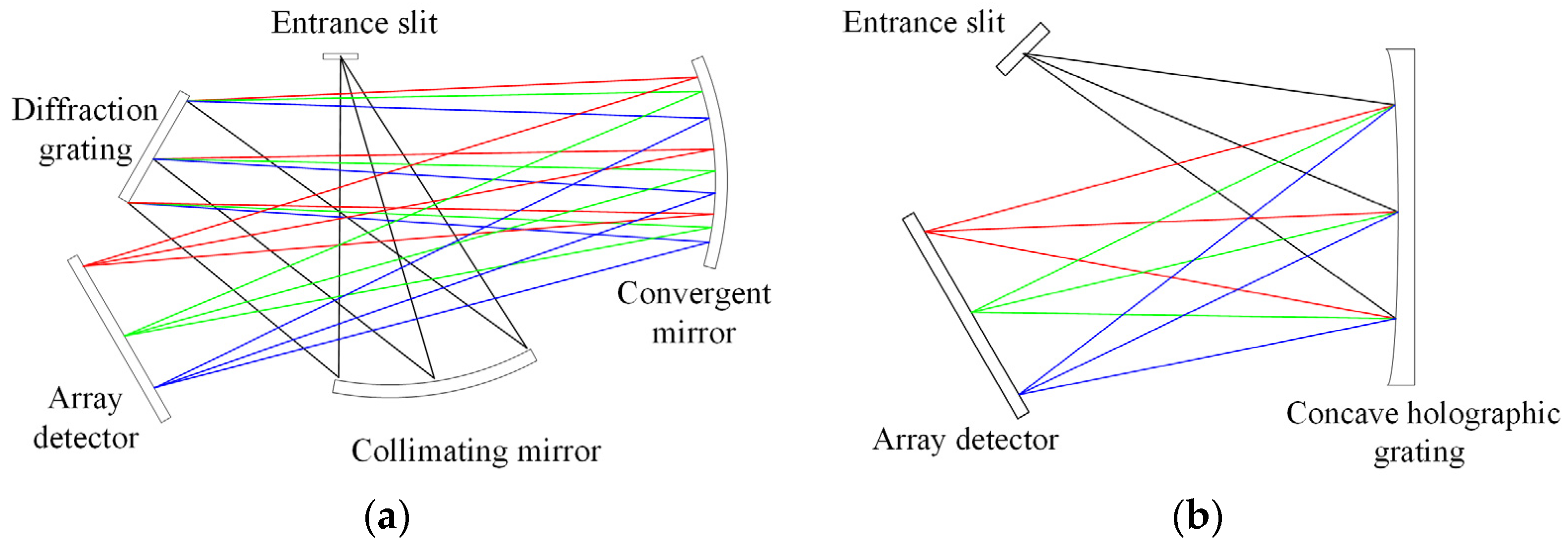
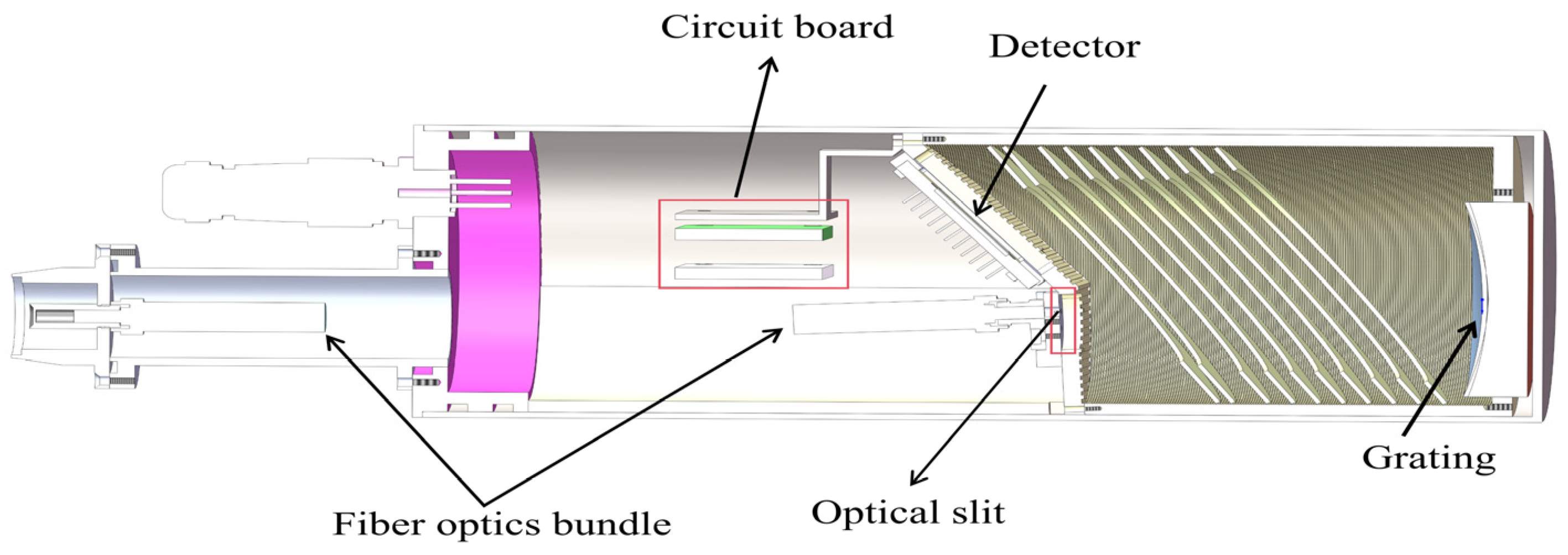
3.3. Spectrometer System Design

The spectrometer system is the core component of the underwater spectral radiometer and is essentially a miniature spectrometer module. This instrument is mainly used for underwater spectral radiation measurements. Considering relevant instruments at home and abroad, as well as the characteristics of underwater “optical windows” and signal-to-noise ratio requirements, the performance specifications of the instrument are proposed. The spectral range of this spectrometer is 400–950 nm. For in situ measurement of underwater spectral radiation, a spectral resolution of 5–10 nm is sufficient to capture the spectral radiation in water. However, for sharp spectral features, it may not be enough [17]. Therefore, this design specifies a spectral resolution better than 3 nm to address this issue.

As shown in Figure 3, there are two commonly used structures for micro-spectrum: one is plane grating C-T (Czerny-Turner) structure, and the other is based on field holographic concave grating structure.

This design uses a flat-field concave holographic grating as the dispersive element of the spectrometer. Compared with miniature spectrometers with a C-T structure, the selected structure is easier to assemble, which is advantageous for a more compact and lightweight design. In addition, the former has a smaller F-number, therefore having a larger light-collecting aperture, which is beneficial for improving the system’s signal-to-noise ratio.

Table 1. Design specifications for a miniature spectrometer optical system.

Parameters	Value
Spectral range/nm	400–950
Diffraction order	+1
Spectral resolution/nm	≤3
Grating density	217 L/mm
Slit width/μm	50
F-number	2.27
Spectrum length/mm	20.2

presents the main parameters of the miniature spectrometer.

As shown in Figure 4, establish a Cartesian coordinate system with O as the origin. The origin O coincides with the center of the grating, the X-axis coincides with the normal to the grating surface, the Y-axis is perpendicular to the direction of the grating lines, and the Z-axis is parallel to the direction of the grating lines. Points C and D are two recording points located in the XOY meridian plane, representing the positions of two relevant point sources for producing the grating. Point A is the position of the light source incidence point, and point B represents the focal point of wavelength $\lambda$ after the light from point A undergoes holographic grating diffraction on the flat-field concave surface. The central main rays CO and DO of the recorded beams emitted from points C and D are, respectively, denoted as $r_C$ and $r_D$ in terms of their lengths. The angles they form with the X-axis are, respectively, denoted as $\gamma$ and $\delta$. The light beam emitted from A with a wavelength of $\lambda$ has a central main ray AO, with a length denoted as $r_A$ and an angle $\alpha$ with the X-axis. After diffraction by the grating, the m-th order diffracted light forms an image at point B on the detector B₁B₂ with the image distance from OB denoted as $r_B$ and the diffraction angle as $\beta$. OH is the perpendicular line from O to the spectrum surface B₁B₂, with a length denoted as $r_H$ and an angle with the X-axis as ${\beta }_H$ [18].

Let P be any point on the plane concave holographic grating. If the light emitted from point A is imaged at point B after passing through point P, then the optical path length of the light ray APB can be represented by Equation (7) as follows:

$$F=AP+PB+n(y,z)m\lambda$$

(7)

In Equation (7), m represents the diffraction order of the grating, and $n(y,z)$ represents the groove number from any point P on the concave grating to the origin point O. It is determined by two coherent point sources C and D.

$$n(y,z)=\frac{1}{{\lambda }_0}\left[(\overrightarrow{CP}-\overrightarrow{DP})-(\overrightarrow{CO}-\overrightarrow{DO})\right]$$

(8)

In Equation (8), ${\lambda }_0$ represents the wavelength of the recording light source, namely, the wavelength of the two coherent point light sources C and D.

If all optical paths from point A to point B through any point of the grating are equal, point A can be accurately focused on point B. Therefore, by substituting Equation (8) into Equation (7) and expanding the optical path function into a power series, we can eventually obtain:

$$F=F_{00}+\mathrm{y}{F}_{10}+\frac{1}{2}{\mathrm{y}}^2{F}_{20}+\frac{1}{2}{\mathrm{y}}^2{F}_{02}+\frac{1}{2}{\mathrm{y}}^3{F}_{30}+\frac{1}{2}{\mathrm{zy}}^2{F}_{12}+\frac{1}{8}{\mathrm{y}}^4{F}_{40}+\frac{1}{4}{\mathrm{y}}^2{\mathrm{z}}^2{F}_{12}+\frac{1}{8}{\mathrm{z}}^2{F}_{04}+\cdots$$

(9)

In Equation (9), $F_{20}$ represents defocus, $F_{02}$ represents astigmatism, $F_{30}$ represents meridional coma, $F_{12}$ represents sagittal coma, and the remaining terms are higher-order aberrations. Each term $F_{ij}$ can be expressed in the following form:

$$F_{ij}=M_{ij}+m\frac{\lambda }{{\lambda }_0}{H}_{ij}$$

(10)

$M_{ij}$ is only related to the parameters used in the structure, while $H_{ij}$ is only related to the parameters used in the manufacture of the structure. Selecting the main aberration coefficients, establish the objective function for minimization:

$$I_{ij}={\displaystyle {\int }_{{\lambda }_2}^{{\lambda }_1}\left(F_{20}^2+F_{02}^2+F_{30}^2+F_{12}^2\right)}d\lambda$$

(11)

Solving the optimal aberration function for the aforementioned flat-field concave holographic grating and transforming it to obtain the optimal parameter values that minimize the aberration expression in Equation (11).

According to Formula (11), the design of flat-field concave holographic gratings is the process of solving the optimal solution to minimize the aberration function value of flat-field concave holographic gratings. In this paper, a genetic algorithm is used to solve the initial values of the design parameters of the plane-field concave grating. When the solution space of the genetic algorithm is close to the global optimal solution, the convergence speed is slow and the convergence accuracy is decreased, which seriously affects the calculation efficiency. Therefore, when the results approach the global optimal solution, the search is stopped, and the incomplete convergence solution is input into the optical tracking software Zemax 19.4 as the initial structural parameters of the flat-field concave holographic grating. The local optimization algorithm of Zemax optical simulation software is used for secondary optimization, and the optimization is stopped when the design indexes are met and the optimal solution of the grating design parameters is finally obtained. The simulated optical system of the spectrometer’s final structure is illustrated in Figure 5, and the specific parameters are listed in

Table 2. Optimization parameters of the flat-field holographic concave grating.

Mounting Parameters		Recording Parameter
$r_A$/mm	84.9	$r_C$/mm	181.44
$\alpha$/(°)	2.5	$\gamma$/(°)	4.13
$r_H$/mm	64	$r_D$/mm	239.14
${\beta }_H$/(°)	40.51	$\delta$/(°)	9.67
R/mm	85.787	$\sigma 1$/μm	4.6

.

The optical imaging quality of the above design results was evaluated using the optical design software Zemax. The resolution of the spectrometer is closely related to the width of the entrance slit, with a larger slit width resulting in lower spectral resolution [19]. The designed spectrometer in this study uses a slit width of 50 μm and a height of 1 mm. Nine coordinates representing the center and edges of the optical slit were selected through ray tracing. Figure 6 illustrates the point plots of the spectrometer around 400, 675, and 950 nm, indicating that the spectrometer’s resolution is better than 3 nm at these three wavelengths.

4. Stray Light Suppression and Simulation Analysis

Stray light is one of the crucial indicators for assessing the performance of optical systems. Factors such as internal reflections on optical surfaces within the spectrometer, defects in the grating, and surface irregularities of optical components can lead to unnecessary distortion in spectral measurements. This becomes a significant source of uncertainty in high-spectral radiometer measurements. Particularly in the context of ocean color measurements, such undesired optical disturbances often contribute significantly to errors in radiance and irradiance measurements, especially in the case of high instrument sensitivity or low signal-to-noise ratios, such as deep-sea and near-infrared spectra. Therefore, to ensure the reliable performance of underwater solar spectrometer systems, it is imperative to conduct stray light analysis and suppression.

4.1. Sources of Stray Light and Inhibition Assessment Methods

The underwater spectral radiometer’s overall opto-mechanical structure is depicted in Figure 7, consisting primarily of the front-end optical system and the spectroscopic system. Solar radiation entering the water is collected by the front-end optical system, guided through fiber optic bundles into the micro-spectrometer module. After passing through an optical slit, the light is diffracted by a flat-field concave holographic grating, and the dispersed spectrum is detected on the surface of the spectroscopic detector. Due to the small size of the optical slit in the micro-spectrometer module and the coupling of light through fiber optics, extraneous stray light outside the field of view entering the micro-spectrometer module is minimal and can be neglected. Therefore, the stray light in the spectrometer mainly originates from light other than the required order diffraction, reaching the detector surface, and is considered as system stray light.

As shown in Figure 8, spectral distributions of different diffraction orders are given. By analyzing the propagation path of light in the micro-spectrometer, it can be inferred that the stray light in this system mainly comes from two sources. The detected wavelength range of the system is 400–950 nm, according to the grating diffraction Equation (12) as follows:

$$m\lambda =d(\sin {\theta }_i\pm \sin {\theta }_d)$$

(12)

In the Equation, m represents the diffraction order, $\lambda$ is the wavelength of the incident light; d is the groove spacing of the grating; ${\theta }_i$ is the angle of incidence; ${\theta }_d$ is the diffraction angle; $\pm$ depends on the positive or negative diffraction order.

From Formula (12), it can be inferred that the second-order diffraction spectrum in the 400–475 nm range of the underwater spectral radiometer will overlap with the first-order diffraction spectrum in the 800–950 nm range on the detector image plane. They cannot be distinguished in the detector pixel space. This part of stray light is referred to as direct stray light, and it severely affects the system, necessitating means to eliminate it. Another portion of stray light results from diffraction orders that are not actively used by the grating. After multiple reflections and scatterings within the optical elements and the mechanical structure’s inner walls of the instrument, this stray light reaches the detector image plane. This type of stray light is known as indirect stray light, and it may be distributed at various locations on the detector surface. For this system, measures must also be taken to suppress this indirect stray light.

When an optical system undergoes stray light suppression design, it is necessary to calculate the stray light energy entering the system and assess the performance of the stray light. The common evaluation methods include measuring the system’s stray light coefficient V, using the Point Source Transmittance (PST) from the stray light model, and conducting radiance distribution analysis. With the accurate design of surface properties for various materials in the simulation model, the stray light coefficient of the system is calculated using radiance distribution analysis graphs output by ray tracing analysis software. This is used to assess the level of stray radiation in the system. Specifically, we represent this performance as the ratio of the energy of stray light radiation $E_S$ from unexpected optical paths to the total energy reaching the image plane $E_T$.

$$V=\frac{E_S}{E_T}$$

(13)

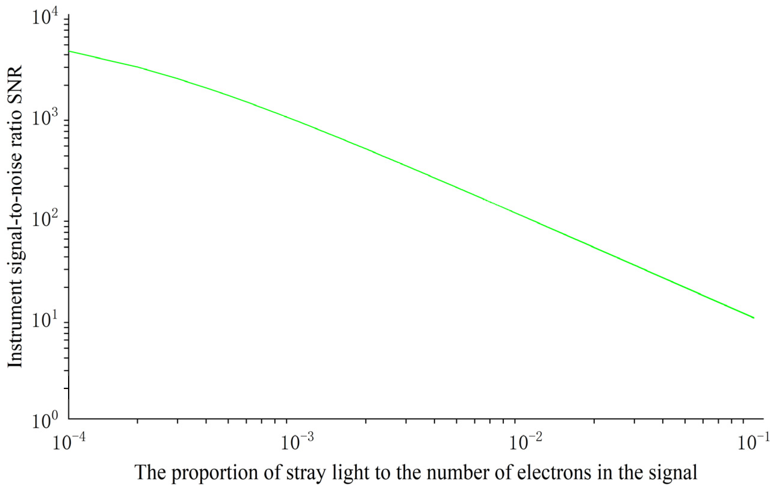
4.2. Analysis and Calculation of Stray Light Suppression Index

According to the theory of radiation transmission in water, assuming $E_S(\lambda )$ represents the spectral irradiance at the sea surface, and $T_s$ is the transmittance at the sea-air interface, the downward spectral irradiance at a depth $z$ below the sea surface is given by the following:

$$E_d(\lambda ,z)=T_s\times E_S(\lambda )e^{-K_d(\lambda )z}$$

(14)

$T_c$ represents the transmittance of the front optical system of the underwater spectral radiometer, entering the spectral irradiance at the entrance pupil of the spectrometer as follows:

$$E_{d1}(\lambda ,z)=T_c\times T_s\times E_S(\lambda )e^{-K_d(\lambda )z}$$

(15)

The entrance radiance of the underwater spectral radiometer would be the following:

$$L_s\left(\lambda \right)=E_{d1}(\lambda ,z)/\pi$$

(16)

F represents the F-number of the optical system, and ${\tau }_o\left(\lambda \right)$ is the grating diffraction efficiency, then the spectral irradiance received by the detector is given by the following:

$$E_d\left(\lambda \right)=\frac{\pi {\tau }_o(\lambda )L_s\left(\lambda \right)}{4F^2}$$

(17)

The area of a detector pixel is denoted by $A_d$, during the integration time $T_{\mathrm{int}}$, the energy received by the detector can be represented as follows:

$$\begin{array}{c}Q(\lambda )=E_d(\lambda )\times A_d\times T_{\mathrm{int}}\times \mathsf{\Delta }\lambda \\ =\frac{\pi {\tau }_o(\lambda )L_s(\lambda )}{4F^2}\times A_d\times T_{\mathrm{int}}\times \mathsf{\Delta }\lambda \end{array}$$

(18)

Considering the quantum efficiency of the detector, the number of photoelectrons generated by the detector during the integration time is given by the following:

$$S_e\left(\lambda \right) =\eta \left(\lambda \right)\times Q\left(\lambda \right)/\left(\frac{hc}{\lambda }\right)$$

(19)

Translating the Equations (14)–(18) into Equation (19), the number of photo-generated electrons in the detector is as follows:

$$S_e\left(\lambda ,z\right) =T_c\times T_s\times \frac{A_d}{4F^2}\times \frac{\lambda }{hc}\times T_{\mathrm{int}}\times {\tau }_o\left(\lambda \right)\times E_S\left(\lambda \right)\times \eta \left(\lambda \right)\times \Delta \lambda \times e^{-K_d(\lambda )z}$$

(20)

where $\eta \left(\lambda \right)$ is the quantum efficiency, and $\Delta \lambda$ is the spectral resolution, $h$ is the Planck constant, and $c$ is the speed of light, the definitions of the remaining quantities are given above.

The detector chosen for this system is a silicon photodiode array. Considering only the detector’s dark current noise, the signal-to-noise ratio of the underwater spectral radiometer is as follows:

$$SN{R}_1=\frac{S_e}{\sqrt{S_e+N_{dark}^2}}$$

(21)

Equation (22) gives the specific expression for dark current noise as follows:

$$N_{dark}=\frac{I_{dark}\times T_{\mathrm{int}}}{q}$$

(22)

Let $S_R$ be the number of electrons generated by stray light. The method for calculating the signal-to-noise ratio of the optical system under the influence of stray light is as follows:

$$SNR=\frac{S_e}{S_R+\sqrt{S_e+N_{dark}^2}}$$

(23)

In Ocean Class I water bodies, the 490 nm wavelength of light holds significant importance in aquatic observations, particularly due to its close correlation with the optical properties and biological relevance of water. Taking the downward spectral irradiance of sunlight at 490 nm in oceanic water as an example, analyzing the relationship between the signal-to-noise ratio of the system and the proportion of stray light, the relevant parameters are as follows:

• The solar zenith angle is 0 degrees.
• Surface solar spectral irradiance $E_S(490)=1.2 {\mathrm{w}/\mathrm{cm}}^2.\mathsf{\mu }\mathrm{m}$
• Air-to-sea interface transmittance $T_s=0.98$
• Diffuse attenuation coefficient in oceanic-type water $K(490)={0.05 \mathrm{m}}^{-1}$
• The instrument’s position below the sea surface is z = 20 m
• Pixel area $A_{\mathrm{d}}=2.5 \mathrm{mm}\times 25 \mathsf{\mu }\mathrm{m}$; Quantum efficiency $\eta \left(\lambda \right)=0.5$
• The transmittance of the optical system for irradiance measurement: $T_{\mathrm{c}}=0.02\%$

$T_c$ is the result of the cosine corrector transmittance combined with fiber optic bundle coupling.

• Grating diffraction efficiency ${\tau }_o\left(\lambda \right)=0.4$
• Detector dark current $I_{dark}=0.3\mathrm{pA}$

When the proportion of stray light to signal light changes during an integration time of 1 s, the variation in the system’s signal-to-noise ratio is as shown in Figure 9.

From Figure 9, it can be observed that when the stray light signal is less than 1% of the signal light magnitude, the signal-to-noise ratio of the underwater spectral radiometer exceeds 10², meeting the instrument’s design requirements.

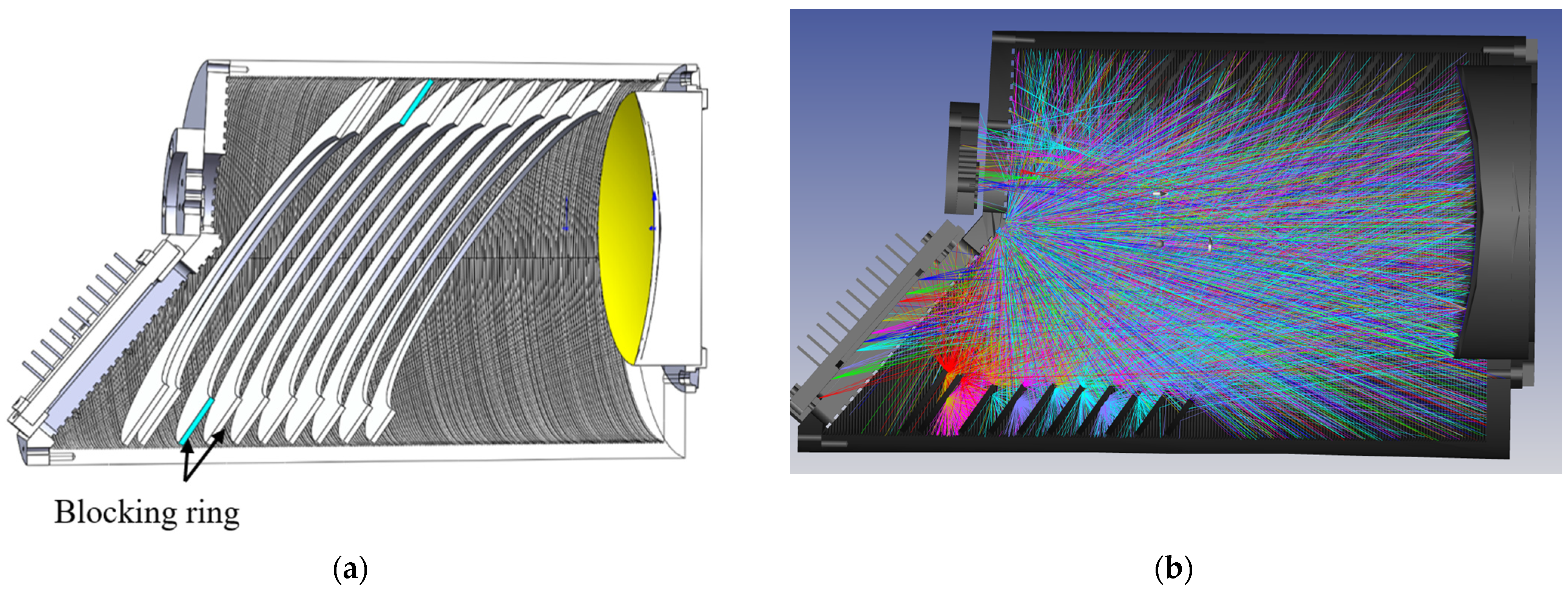
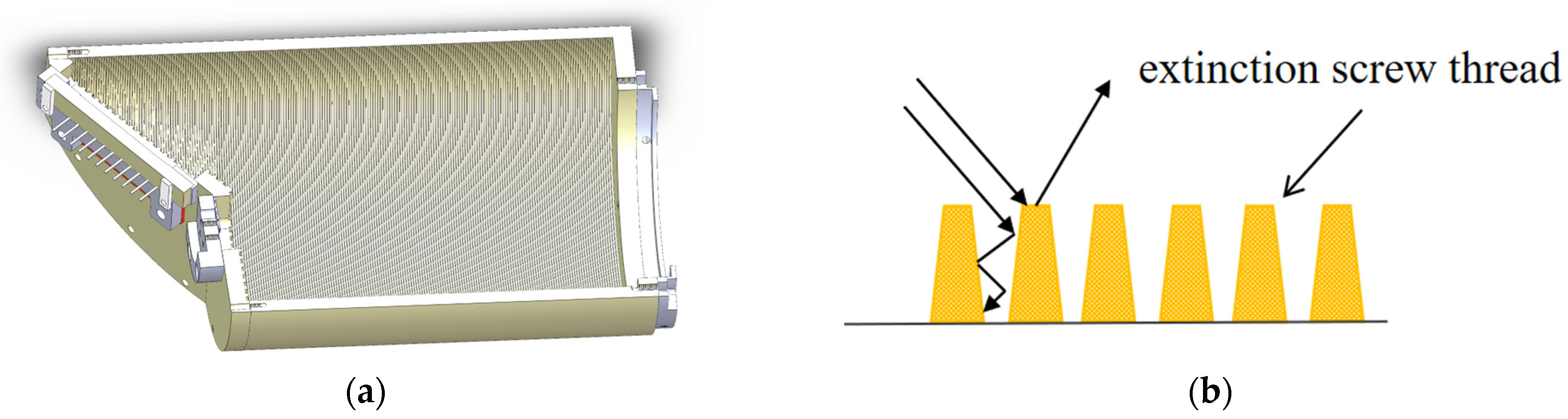
4.3. Stray Light Suppression Methods

According to the grating diffraction equation, the second-order diffraction spectrum in the 400–475 nm range overlaps with the first-order diffraction spectrum in the 800–950 nm range, sharing the same diffraction angle, and directly falls onto the image plane of the detector, Figure 10a shows the spectral overlap on the detector. To mitigate the interference from this portion of stray light, based on the optical system simulation results, the distribution area where the second-order diffraction spectrum overlaps on the detector surface was determined, and the specific mapping positions of wavelengths on the detector are illustrated in Figure 10b. A long-wave bandpass film was applied to the optical window surface corresponding to this area to eliminate the impact of the short-wave second-order spectra.

Although the light of other diffraction orders and the remaining spectrum of the second-order diffraction spectrum cannot directly reach the detector surface, a considerable part of the light will still reach the detector surface after repeated reflections from the optical and mechanical components of the spectrometer. Through optical tracing, the key surface of the source of stray light in the optical system can be found, and the extinction thread is designed to roughen the mechanical surface, so as to reflect or scatter on the mechanical surface to prevent stray light from falling on the detector surface [20]. The physical picture of the extinction thread and the principle diagram of the extinction screw thread to suppress stray light are shown in Figure 11.

In order to further prevent stray light from entering the optical system, several light baffles (light stops) are installed within the shading hood. The function of the light baffle is to completely eliminate primary stray light. The stray light entering the light baffle is blocked and absorbed by the inner walls, while the remaining stray light is reflected into adjacent light baffles to block it. In this way, primary stray light is completely eliminated before entering the optical lens. The light baffles and the walls of the shading hood together form a semi-enclosed light trap, which is used to block the transmission path of indirect stray light (reflected light, scattered light) and reduce the transmission energy multiple times. This is particularly effective for stray light at large angles outside the axis [21]. Figure 12b is a schematic diagram of light ray tracing after adding the light-shielding ring.

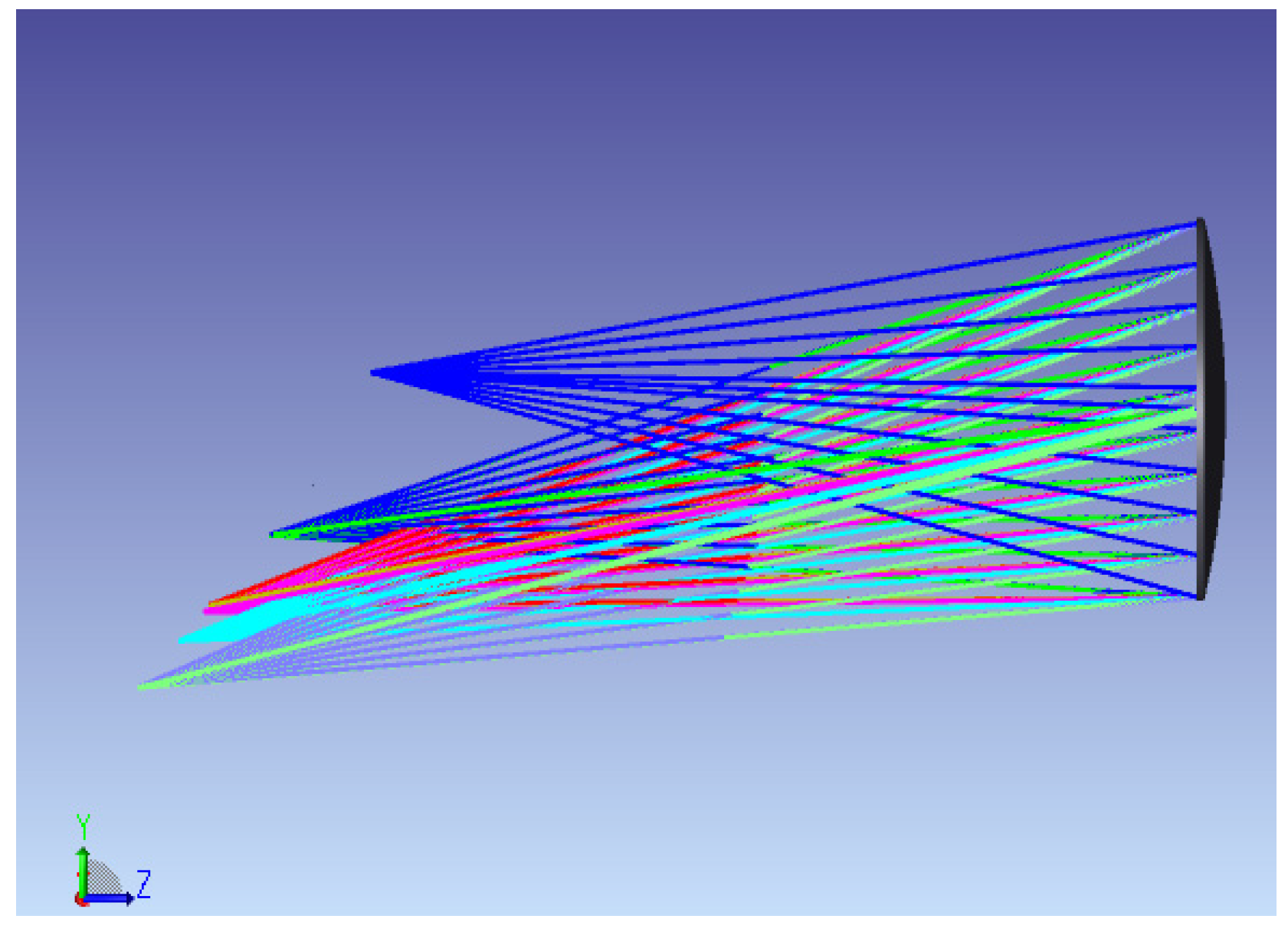
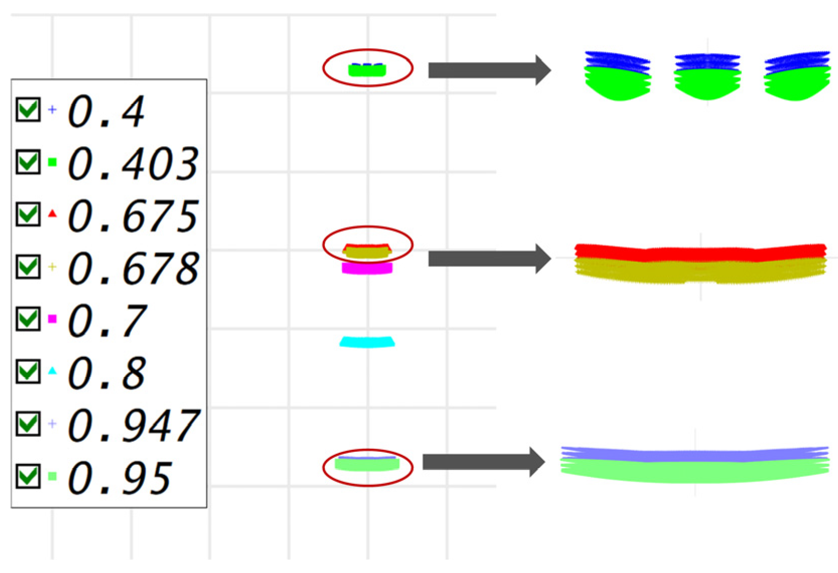
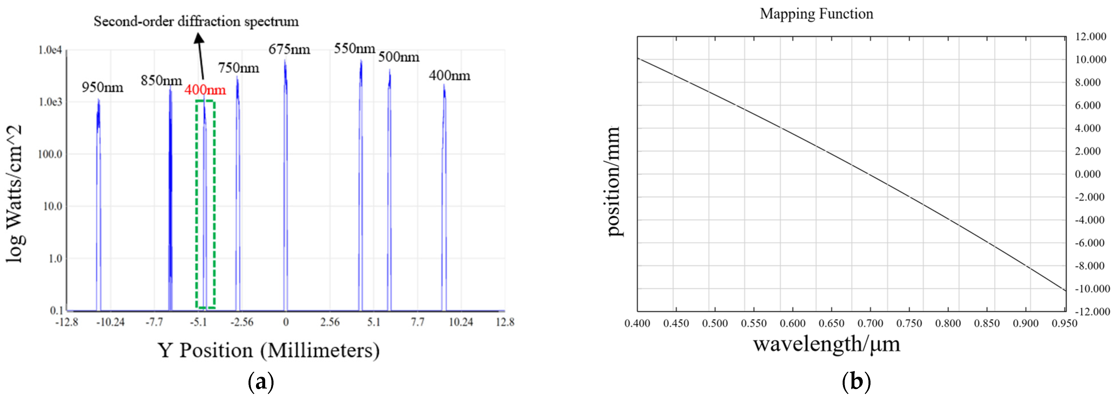
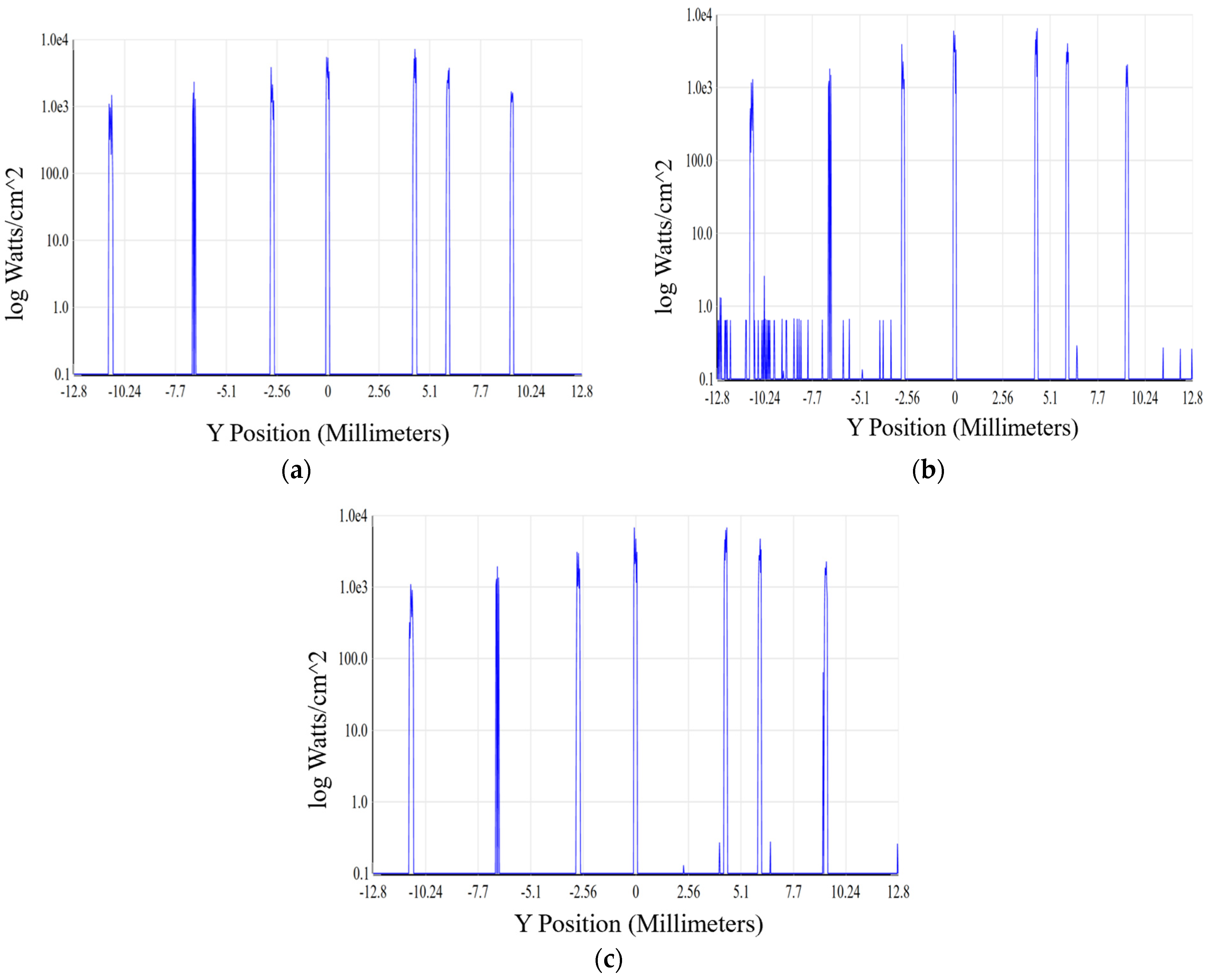
4.4. Simulation Results Analysis

The ray tracing is based on the principles of geometric optics and optical laws, simulating the propagation of light rays within optical systems to achieve research and analysis of the performance and behavior of optical systems. The non-sequential mode is a more rigorous method of geometric ray tracing. In this mode, the scattering, reflection, and absorption processes of light on object surfaces are fully considered. Therefore, simulation analysis of stray light in instruments is typically based on the non-sequential mode. According to the system simulation parameters, ray tracing of the optical and mechanical structure of the spectrometer module was carried out in Zemax with a non-sequential structure. The total diffraction efficiency of the grating is 90%, with the main diffraction orders being −1, 0, +1, and +2, and their respective proportions being 1:2:4:2. Other diffracted light is scattered and absorbed. Other critical surfaces undergo blackening treatment, with a surface absorptance of 90% and a Lambertian scattering model with a scattering function of 0.8. Nine light sources are placed at positions corresponding to the slit size to characterize the incident light within the entire slit area. The energy of each of the nine light sources is 1 W. The ray tracing relative threshold is set to 1.0 × 10⁻⁸.

As shown in Figure 13, the cross-section analysis diagram of the detector surface irradiance under the different configurations of the spectrometer is given. The peak wavelength in the diagram represents the seven target wavelengths set during the optical tracing process, and the other small peaks represent the distribution of stray light. Figure 13a shows the irradiance distribution of the detector surface under ideal conditions, and Figure 13b shows the irradiance of the detector surface after the mechanical structure surface is blackened. It is worth noting that compared with the ideal optical system, the detector also receives a considerable amount of stray light in addition to receiving signals from the target wavelength. Figure 13c shows the distribution of stray light on the detector surface after extinction threading and the addition of blocking ring treatment on the mechanical inner surface of the spectrometer (see Figure 12 for the specific mechanical structure). Compared with the smooth surface only after blackening, the stray light suppression level is significantly improved, and the stray radiation of the spectrometer can be controlled at the order of 10⁻⁴. The influence of stray light on the system is reduced, and the effect of stray light suppression meets the design requirements of the system.

5. Experiment and Results

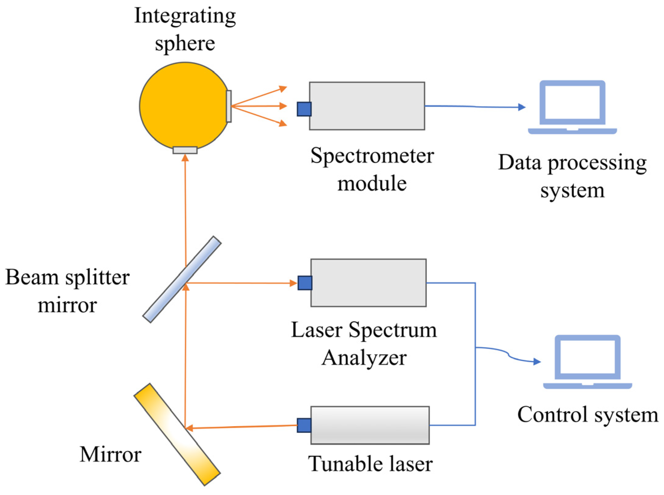
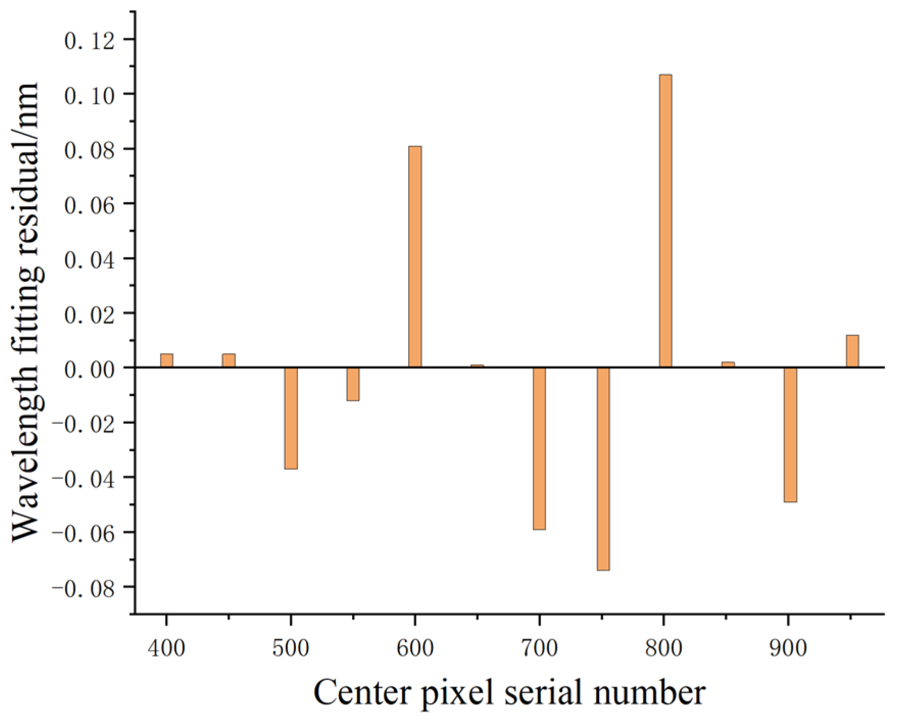
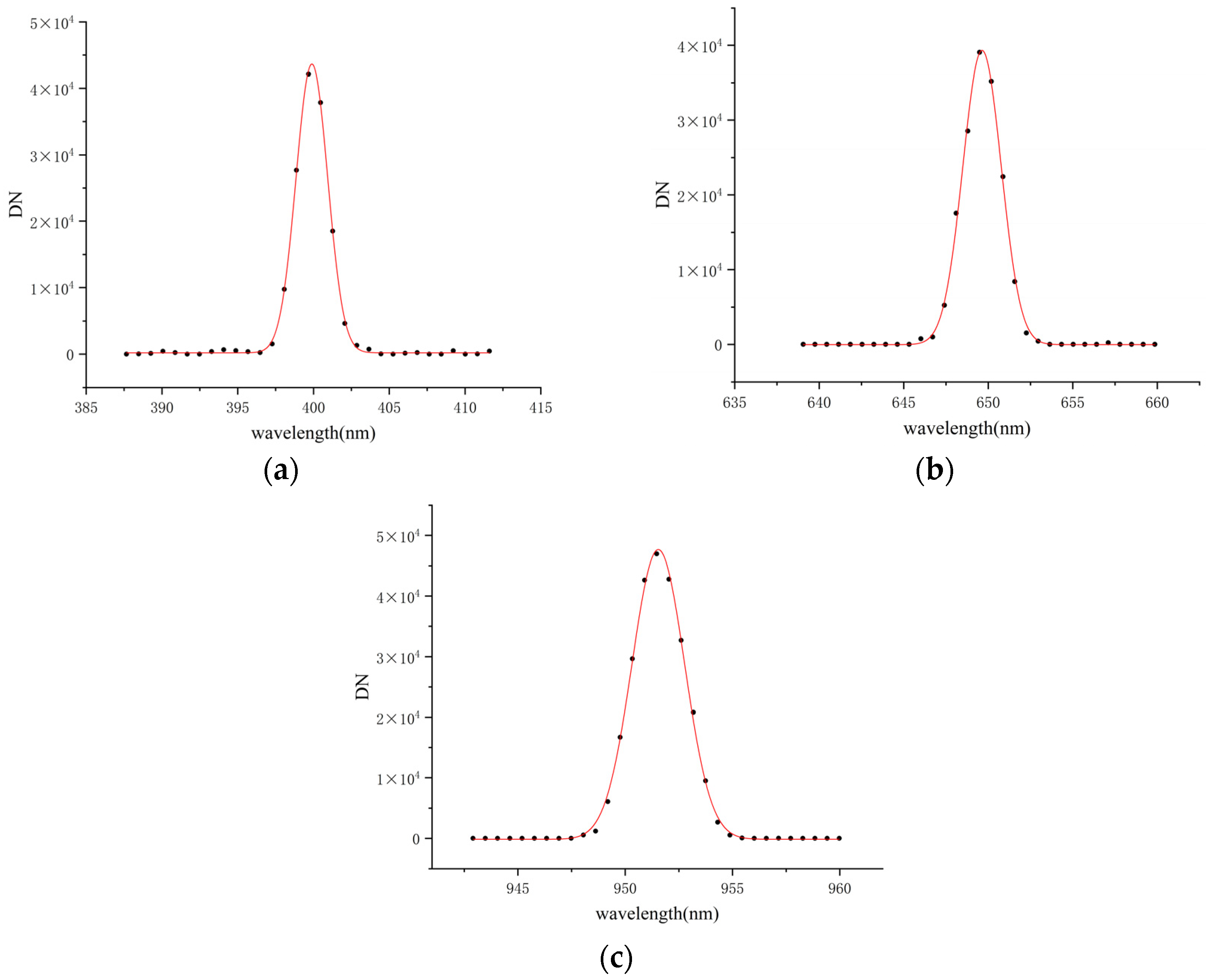
5.1. Wavelength Calibration

A tunable laser was used to calibrate the laboratory spectrum of an underwater spectrometer. The tunable laser adopts EKSPLA NT242, which can output a continuously tunable laser wavelength in the spectral range of 210–2600 nm, covering all bands required for wavelength calibration. The repetition frequency of the laser is 1 kHz, and the line width is better than 5 cm⁻¹. In the process of spectral calibration, the laser spectrum analyzer is used to monitor the change in laser output wavelength. The spectral calibration system is shown in Figure 14. After passing through the reflector, the Laser beam is divided by the beam splitter, one beam enters the Laser Spectrum Analyzer (LSA) for wavelength monitoring, the wavelength measurement accuracy is better than 0.01 nm, and the other beam passes through the integrating sphere and is measured by the underwater spectrometer. The main control computer controls the switching of the laser wavelength and the data acquisition of the spectrometer. Once the laser’s output wavelength stabilizes, the measurement parameters from the laser spectrum analyzer are read, providing the true emission wavelength of the laser.

Based on the spectral mode of the underwater spectrometer, the dispersion has a certain uniformity. Twelve groups of spectral lines were selected equally in 400–950 nm for wavelength calibration. For the measurement of each beam of monochromatic light, the corresponding pixel position is obtained by Gaussian fitting of the response value of each spectral channel, and the corresponding relationship between the spectral pixel number and the detection wavelength is determined. Specific data are shown in

Table 3. Mapping between wavelength and pixel serial number.

Numerical Order	Wavelength/nm	Central Pixel
1	399.916	132.298
2	449.895	195.813
3	499.849	261.162
4	549.789	328.254
5	599.740	397.166
6	649.612	468.180
7	699.526	541.292
8	751.034	618.966
9	801.193	696.694
10	851.443	777.586
11	901.524	860.939
12	951.564	947.142

.

The wavelength and central pixel in the above table were fitted by using the origin. After multiple fitting analyses, the residual sum of squares of the 5th-degree polynomial fitting was the smallest, so the 5th-degree polynomial was chosen as the final fitting result. The specific expression is shown as follows:

$$\begin{array}{l}\lambda =1.13536\times {10}^{-14}{n}^5-5.12284\times {10}^{-11}{n}^4+9.32479\times {10}^{-8}{n}^3- 2.13197\times {10}^{-4}{n}^2\\ +0.85011n+290.97428\end{array}$$

(24)

Figure 15 shows the histogram of the residual distribution of the quintic multinomial fitting model. Fitting residuals of 12 calibration wavelengths are given. The results show that the wavelength scaling residuals of the center coordinates fitted by Gaussian are distributed within ±0.11 nm.

After the wavelength calibration, the spectral resolution of the underwater spectrometer is verified. As shown in Figure 16, the response code values of each spectral channel and the half-peak full width of the response curve can be expressed as the spectral resolution of the spectrometer at this wavelength when three groups of specific wavelengths of monochromatic light incident.

According to

Table 4. Spectrometer calibration wavelength and spectral resolution.

WAVE/nm	FWHM/nm
399.902	2.458
449.918	2.688
499.862	2.891
549.795	2.805
599.634	2.823
649.584	2.670
699.513	2.432
751.032	2.362
801.181	2.217
851.428	2.272
901.501	2.422
951.597	2.869

, the spectral resolution of the spectroradiometer at 400–950 nm is better than 3 nm.

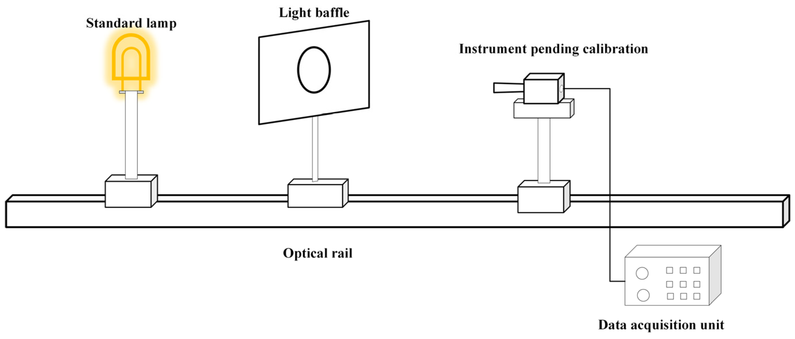
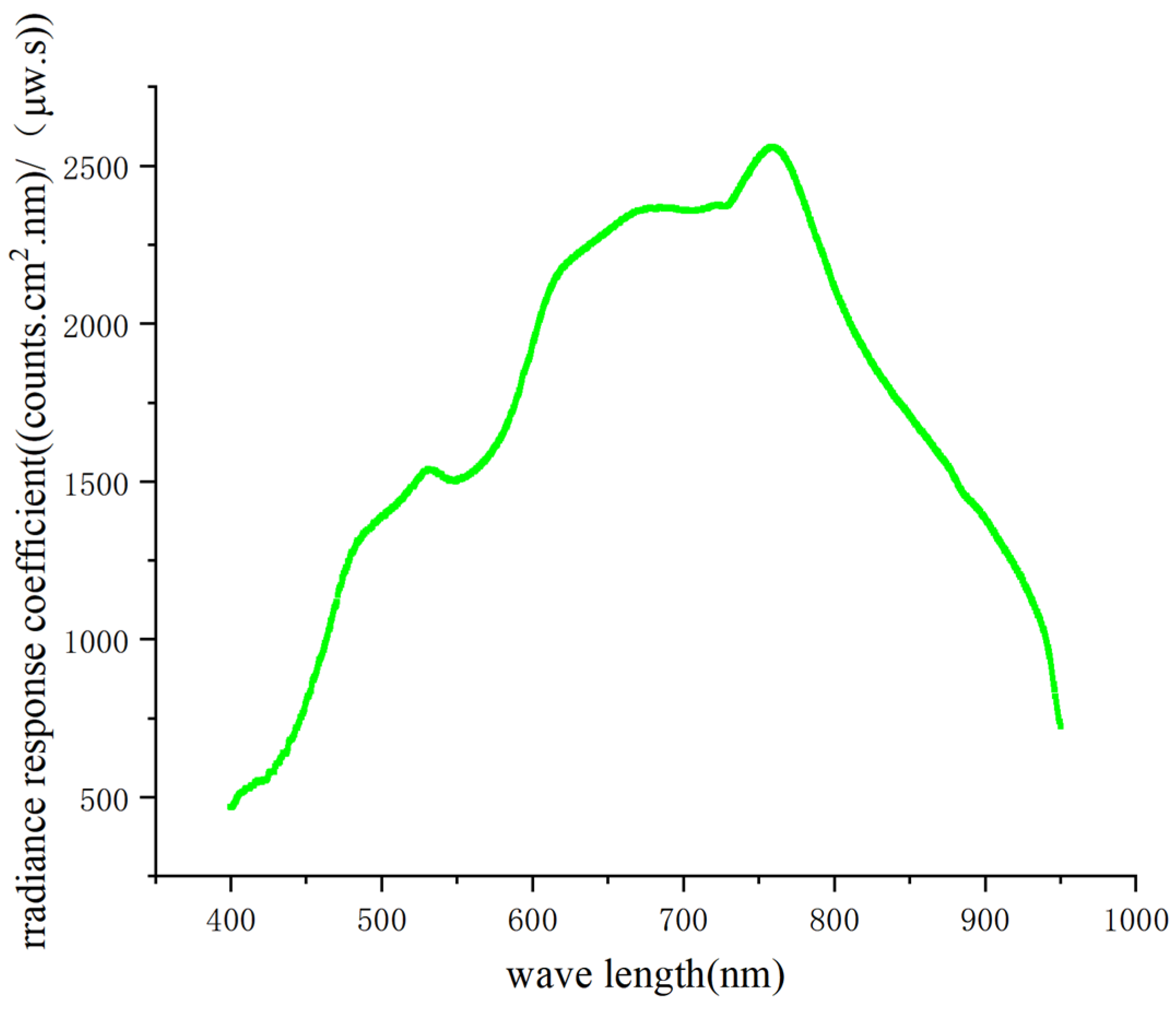
5.2. Radiometric Calibration

The underwater spectrometer is calibrated in the laboratory by the standard irradiation lamp calibration method. The standard lamp used is a 1000 W quartz halogen tungsten lamp, whose spectral range covers the measurement band of the underwater spectrometer and whose spectral irradiance can be traced to the national high-temperature blackbody radiation reference source. The irradiance calibration using standard lamps is shown in Figure 17. The standard irradiance lamp uses the standard constant-current power supply to provide the calibration light source according to the measurement specification, and the underwater spectrometer is measured at the standard distance. The distance measurement uses the horizontal laser rangefinder, which not only ensures collimation but also provides a distance measurement accuracy better than 1 mm. An anti-stray stop wrapped in black cloth is placed between the spectrometer and the calibration light source, and the experiment is completed in the optical darkroom to achieve the suppression of space stray light and reduce the error introduced by it to the calibration.

The spectral irradiance response coefficient $R(\lambda )$ can be obtained by calibrating the quantitative relationship between the output value and the incident spectral irradiance of the instrument at different wavelengths. The corresponding expression is shown in Formula (25):

$$R(\lambda )=\frac{S(\lambda )}{E(\lambda )}$$

(25)

$E(\lambda )$ represents the spectral irradiance of the standard lamp at the response wavelength, and $S(\lambda )$ is the normalized function of the detector output signal. The spectral responsiveness curve obtained according to the above formula is shown in Figure 18.

5.3. Uncertainty Analysis

From Equation (25), it can be seen that the uncertainty sources in laboratory radiation calibration mainly include the uncertainty of the calibration source itself and the uncertainty introduced by instrument measurements. The uncertainty of the calibration source is provided by the calibration certificate, and by consulting the calibration certificate, it can be determined that the uncertainty of the spectral irradiance of the calibration source is better than 1% in the range of 400–950 nm. The uncertainty of the spectral irradiance caused by the stable current driving the spectral irradiance standard lamp is 0.1%.

The spectral irradiance received by the instrument is influenced by the distance between the instrument and the standard lamp, following the inverse square law. Utilizing a high-precision laser ranging sensor to measure the distance between the center of the filament of the standard lamp and the optical detection point of the instrument, when the distance between them is 500 mm, the maximum error value observed during three measurement sessions is 1 mm. Hence, the uncertainty caused by the calibration distance is less than 0.4%.

During spectral irradiance calibration, the calibration device is placed on an optical experimental platform. The reflection of light from the optical experimental platform and other instruments entering the probe of the spectral radiometer is one of the important sources of spatial background stray light. To assess the impact of this stray radiation on measurement results, first, the standard lamp is observed using the spectral radiometer, and the output code value of the radiometer is recorded. Then, the standard lamp light source is blocked using a black shield, and the output code value of the instrument is recorded currently. The ratio of these two measurement results represents the response of the radiometer caused by spatial background stray light. For this calibration system, the uncertainty introduced by spatial background stray light is approximately 0.2%.

The measurement stability of the spectral radiometer system is primarily influenced by the signal-to-noise ratio (SNR) of the output signal, which is determined by the relative standard deviation of multiple measurements during calibration (measurement standard deviation/measurement mean). By taking multiple measurements of the calibration light source within a short period of time to obtain the sample’s mean and standard deviation, the signal-to-noise ratio (SNR) of the instrument, denoted as $R_{SN}$, can be represented by Equation (26). The reciprocal of the signal-to-noise ratio represents the uncertainty introduced by the system noise.

$$R_{SN}=\frac{x_p}{S_{\sigma }}$$

(26)

In the above equation, $x_p$ represents the mean value of the sample data, and $S_{\sigma }$ represents the standard deviation of the sample data. According to the evaluation, the calibration uncertainty introduced by the system noise is about 0.3~0.9% in the calibration band. According to the uncertainty synthesis formula, the laboratory calibration uncertainty of the instrument ranges from 1.14% to 1.42% in the 400–950 nm band. The uncertainties of irradiance calibration of underwater spectroradiometer are shown in

Table 5. Irradiance calibration uncertainty.

Uncertainty Sources	Uncertainty
Standard light spectrum irradiance	1%
Stabilized current supply	0.1%
Calibration distance and angle	0.4%
Spatial stray light	0.2%
System noise	0.3~0.9%
Combined uncertainty	1.14~1.42%

.

6. Conclusions

The text describes the design of an in situ underwater spectral radiometer for remote sensing of water color. The system uses a concave holographic grating as a dispersive element, enabling spectral observations within the range of 400–950 nm with a spectral resolution better than 3 nm. The mechanical structure of the underwater spectral radiometer has been completed, employing a method that bonds the grating to a watertight casing, reducing unnecessary mechanical components and ensuring a compact and lightweight design. Furthermore, utilizing Zemax non-sequential mode, stray light analysis has been conducted for the underwater solar spectral radiometer to provide means for stray light suppression. Various methods have been employed, including coating the detector surface with a layer, blackening critical mechanical surfaces, adding light-absorbing threads on the inner wall, and increasing the shading hood. These measures effectively suppress stray radiation to the order of 10⁻⁴, significantly reducing the system’s stray light signal and improving the system’s signal-to-noise ratio. The prototype was developed, and wavelength calibration experiments were carried out with a tunable laser. The experimental results show that the spectral resolution of the instrument meets the design requirements. The spectral irradiance calibration experiment is carried out to obtain the spectral response characteristic curve of the detector, which provides data support for underwater experiments.

References

1. Lin, C.; Yang, H.; Chen, Y.; Jin, X.; Chen, B.; Li, W.; Ren, Z.; Leng, S.; Ding, D. Modern Marine pasture construction and de-velopment—the academic review of the 230th Double Qing Forum. Sci. Found. China 2021, 35, 143–152. [Google Scholar] [CrossRef]
2. Zhang, Y.; Qin, B.; Chen, W.; Gao, G.; Chen, Y. Experimental study on underwater light intensity and primary productivity caused by variation of total suspended matter. Adv. Water Sci. 2004, 15, 615–620. [Google Scholar] [CrossRef]
3. Siegel, D.A.; Westberry, T.K.; O’Brien, M.C.; Nelson, N.B.; Michaels, A.F.; Morrison, J.R.; Scott, A.; Caporelli, E.A.; Sorensen, J.C.; Maritorena, S.; et al. Bio-Optical Modeling of Primary Production on Regional Scales: The Bermuda BioOptics Project. Deep Sea Res. Part II Top. Stud. Oceanogr. 2001, 48, 1865–1896. [Google Scholar] [CrossRef]
4. Zhang, T.; Chen, S.; Xue, C. Research progress of optical properties measurement technology of Marine water body. Atmos-Pheric Environ. Opt. 2020, 15, 23–39. [Google Scholar] [CrossRef]
5. Tian, L.; Li, S.; Sun, X.; Tong, R.; Song, Q.; Li, Y.; Sun, Z. Development of a Floating Water Spectral Measurement System Based on Sky Light Occlusion Method. Spectrosc. Spectr. Anal. 2020, 40, 2756. [Google Scholar] [CrossRef]
6. Li, W.; Tian, L.; Guo, S.; Li, J.; Sun, Z.; Zhang, L. An Automatic Stationary Water Color Parameters Observation System for Shallow Waters: Designment and Applications. Sensors 2019, 19, 4360. [Google Scholar] [CrossRef] [PubMed]
7. Braga, F.; Fabbretto, A.; Vanhellemont, Q.; Bresciani, M.; Giardino, C.; Scarpa, G.M.; Manfè, G.; Concha, J.A.; Brando, V.E. Assessment of PRISMA Water Reflectance Using Autonomous Hyperspectral Radiometry. ISPRS J. Photogramm. Remote Sens. 2022, 192, 99–114. [Google Scholar] [CrossRef]
8. Zhang, X.; Li, C.; Zhou, W.; Liu, C.; Xu, Z.; Cao, W.; Yang, Y. Research on the Diffuse Attenuation Coefficient in the South China Sea Based on Volume Scattering Function and Absorption Coefficient. J. Trop. Oceanogr. 2023, 42, 86–95. [Google Scholar]
9. Li, X. Water-related optics. Sci. Sin. Informationis 2024, 54, 227. [Google Scholar] [CrossRef]
10. de Sa, E.S.; Desa, B.A.E. Design of an In-Water Spectrograph for Irradiance Measurements in the Ocean. Opt. Eng. 1991, 30, 1576–1582. [Google Scholar] [CrossRef]
11. Cao, W.; Guo, Y.; Yang, Y.; Ke, T.; Jin, X.; Yu, B.; Zhong, Q. Multiband Underwater Spectral Radiometer. High-Tech. Commun. 2002, 12, 96–101. [Google Scholar] [CrossRef]
12. Shang, Z.; Lee, Z.; Dong, Q.; Wei, J. Self-Shading Associated with a Skylight-Blocked Approach System for the Measurement of Water-Leaving Radiance and Its Correction. Appl. Opt. 2017, 56, 7033–7040. [Google Scholar] [CrossRef] [PubMed]
13. Gordon, H.R.; Ding, K. Self-Shading of in-Water Optical Instruments. Limnol. Oceanogr. 1992, 37, 491–500. [Google Scholar] [CrossRef]
14. Wu, T.; Cao, W. Research on the Shadow Effect and Its Correction Method in Underwater Radiance Measurements. Acta Oceanol. Sin. 2003, 25, 42–51. [Google Scholar]
15. Li, C.; Ke, T.; Cao, W.; Yang, Y.; Lu, G.; Guo, C.; Deng, C. Design of an anchor chain-type underwater multispectral radiometer. Opt. Tech. 2004, 30, 665–668. [Google Scholar] [CrossRef]
16. Wang, X.; Li, Z. Design and Performance Test of Gershun Tube Spectral Radiometer. Acta Opt. Sin. 2017, 37, 0612002. [Google Scholar] [CrossRef]
17. Ramkilowan, A.; Chetty, N.; Lysko, M.; Griffith, D. Optical Detectors for Integration into a Low Cost Radiometric Device for In-Water Applications: A Feasibility Study. J. Indian Soc. Remote Sens. 2013, 41, 531–538. [Google Scholar] [CrossRef]
18. Wu, J.; Zhao, L.; Chen, Y.; Zhou, C.; Wang, T.; Wang, Y. Design of Wide-Spectrum High-Resolution Flat-Field Concave Holo-graphic Grating Spectrometer. Acta Opt. Sin. 2012, 32, 83–87. [Google Scholar]
19. Kong, P.; Tang, Y.; Bayin Heg Li, W.; Cui, J. Optimal design of zero-astigmatism wide-band flat field holographic concave grating. Spectrosc. Spectr. Anal. 2012, 32, 565–569. [Google Scholar] [CrossRef]
20. Shu, Z.; Han, Z.; Wu, Y.; Lin, Z.; Zhang, H.; Wang, M. Stray light analysis and optimization design for optical system of space detection camera. Appl. Opt. 2023, 44, 982–991. [Google Scholar] [CrossRef]
21. Wang, H.; Chen, Q.; Ma, Z.; Yan, H.; Lin, S.; Xue, Y. Development and Prospects of Stray Light Suppression and Evaluation Techniques (Invited). Acta Photonica Sin. 2022, 51, 56. [Google Scholar] [CrossRef]
Figure 1. Self-shadow in the instrument field of view.
Applsci 14 03172 g001
Figure 2. The overall structure of the underwater spectral radiometer.
Applsci 14 03172 g002
Figure 3. Common structure of a miniature spectrometer. (a) Cross-type C-T structure; (b) Flat-field concave holographic grating structure.
Applsci 14 03172 g003
Figure 4. Flat-field concave holographic grating light path.
Applsci 14 03172 g004
Figure 5. Micro-spectrometer optical path diagram.
Applsci 14 03172 g005
Figure 6. Micro-spectrometer full-field point array diagram.
Applsci 14 03172 g006
Figure 7. The mechanical structure of the underwater spectral radiometer.
Applsci 14 03172 g007
Figure 8. Distribution of various diffraction orders. (a) Distribution of +1 order diffraction light; (b) Distribution of 0 order diffraction light; (c) Distribution of −1 order diffraction light; (d) Distribution of +2 order diffraction light.
Applsci 14 03172 g008
Figure 9. Stray light-to-signal electron ratio and its relationship with signal-to-noise ratio.
Applsci 14 03172 g009
Figure 10. (a) The phenomenon of overlapping second-order spectra in a grating; (b) Mapping of wavelengths onto the detector.
Applsci 14 03172 g010
Figure 11. (a) Design of the structure for the extinction screw; (b) Schematic diagram of the extinction screw.
Applsci 14 03172 g011
Figure 12. (a) Light-shielding ring structure. (b) Ray tracing diagram after adding the light-shielding ring.
Applsci 14 03172 g012
Figure 13. Irradiance received by the detector. (a) The irradiance on the detector surface in an ideal optical system; (b) The irradiance on the detector surface after surface blackening treatment; (c) The irradiance on the detector surface after adding the extinction screw thread and the light-shielding ring.
Applsci 14 03172 g013
Figure 14. Wavelength calibration system.
Applsci 14 03172 g014
Figure 15. Wavelength residual distribution histogram.
Applsci 14 03172 g015
Figure 16. Spectral bandwidths. (a) Spectral bandwidth at wavelength 400 nm. (b) Spectral bandwidth at wavelength 650 nm. (c) Spectral bandwidth at wavelength 950 nm.
Applsci 14 03172 g016
Figure 17. Schematic diagram of spectral irradiance calibration for standard lamp.
Applsci 14 03172 g017
Figure 18. Spectral irradiance scaling coefficient curve.
Applsci 14 03172 g018