Abstract
Unemployment, a significant economic and social challenge, triggers repercussions that affect individual workers and companies, generating a national economic impact. Forecasting the unemployment rate becomes essential for policymakers, allowing them to make short-term estimates, assess economic health, and make informed monetary policy decisions. This paper proposes the innovative GA-LSTM method, which fuses an LSTM neural network with a genetic algorithm to address challenges in unemployment prediction. Effective parameter determination in recurrent neural networks is crucial and a well-known challenge. The research uses the LSTM neural network to overcome complexities and nonlinearities in unemployment predictions, complementing it with a genetic algorithm to optimize the parameters. The central objective is to evaluate recurrent neural network models by comparing them with GA-LSTM to identify the most appropriate model for predicting unemployment in Ecuador using monthly data collected by various organizations. The results demonstrate that the hybrid GA-LSTM model outperforms traditional approaches, such as BiLSTM and GRU, on various performance metrics. This finding suggests that the combination of the predictive power of LSTM with the optimization capacity of the genetic algorithm offers a robust and effective solution to address the complexity of predicting unemployment in Ecuador.
1. Introduction
The unemployment rate is a crucial indicator for evaluating economic activity; it is closely linked to a country’s economic cycle and well-being. Its high variability can trigger significant impacts in emerging nations, and a high unemployment rate can cause contraction, recession, or depression in emerging economies [1]. Despite the complexity associated with predicting the unemployment rate, this key indicator must be considered, as its values allow for assessing a nation’s economic health and generate considerable interest in various sectors, including governments, businesses, and researchers.
The unemployment rate prediction emerges as a fundamental tool with multiple strategic applications. This economic indicator is used by various actors in society, including political leaders who use it as a measure that contributes to decision-making and the design of policies aimed at the national economic planning of a country; human resource managers for the development of appropriate policies related to human resources; financial analysts for the prediction of the economic trend of a target market; foreign investors seeking to invest in a country that provides political, social, and economic stability; as well as the general public, interested in knowing the health of a particular economy.
The need to predict the unemployment rate arises from the importance of this indicator in the economic, political, and social spheres. Economically, unemployment trends can indicate changes in labor demand, financial stability, and consumption; politically, these figures can influence the approval or rejection of government policies and the public’s confidence in institutions; and in the social sphere, unemployment can generate tensions and challenges in community cohesion, affecting the quality of life and general well-being. Understanding and anticipating unemployment trends is essential to implementing effective measures to mitigate their adverse effects, such as developing job training programs, promoting employment opportunities, and protecting workers’ rights. In this sense, the complexity inherent to this prediction process, especially in non-stationary and nonlinear economic environments, requires advanced and flexible intelligent approaches [2]. In recent years, various approaches to predicting the unemployment rate have been explored, including statistical models, econometrics, intelligent computational models, and hybrid prediction models; however, in Ecuador, where there is a limited data set in terms of availability and temporal coverage compared to other countries, this presents a significant challenge for adapting the unemployment prediction models to this specific context.
Although significant progress has been made through the correct implementation of predictive models of the unemployment rate, there are gaps in the existing prediction models, such as the ability to accurately capture and anticipate the effects of events even when the data may not fully reflect the reality of the labor market [3]. In order to solve the gap presented, we need to take some actions, such as: (i) selecting the optimal architecture of intelligent models to improve prediction accuracy and managing inherent uncertainty in data (vague and incomplete data); (ii) developing computationally efficient methods to ensure that complex models can handle large sets of reasonable data and execution times for the exploration of new modeling techniques that improve the margin of precision [4]; (iii) and the prediction models should be able to capture the complex dynamics of the labor market and adapt to structural changes in this environment [5].
To effectively adapt models to these specific conditions in the local context [6], this study focuses on developing an unemployment rate prediction model designed specifically for Ecuador. A hybrid approach is proposed that combines recurrent neural networks (RNN), specifically the long short-term memory (LSTM) network approach, with genetic algorithms (GA). This combination allows the complexities of sequential and nonlinear data to be captured, efficiently optimizing model parameters.
Specific research questions guiding this study include: What is the predictive performance of the genetic algorithm with long short-term memory (GA-LSTM), bidirectional LSTM (BiLSTM), and gated recurrent units (GRU) approaches for predicting the unemployment rate in Ecuador? How do the LSTM network parameters determined by the genetic algorithm influence the accuracy of the predictions?
The document is organized as follows: Section 1 describes the introduction; Section 2 relates works; Section 3 describes the methodology and data used to predict the unemployment rate in Ecuador; and Section 4 and Section 5 show the experimental results and discussion. Section 6 concludes and describes the practical implications of the study.
2. Related Works
This section will review related works on models applied to unemployment rate prediction. Macroeconomic data is obtained from various sources, such as government databases, economic firms, banks, and social networks; the latter is used in novel methods for nowcasting economic forecasts and more timely forecasting of economic indicators. For example, Bokanyi. E. et al. [6] demonstrated how unemployment and employment statistics are reflected in daily Twitter activity. Ryu P. [7] used social media data to predict unemployment in South Korea, combining sentiment analysis and grammar tagging with ARIMA, ARIMAX, and ARX models. Furthermore, Vicente M. et al., Pavlicek J., and Kristoufek L. [8,9] showed how the Google Trends index improves unemployment forecasts in Spain and the Visegrad Group, respectively. D’Amuri F. and Marcucci J. [10] found that the Google index (GI) improves quarterly unemployment predictions in the US. Xu W. et al. [11] developed a data mining framework using neural networks (NN) and support vector regressions (SVR) to forecast US unemployment, outperforming traditional forecasting approaches. Other studies have highlighted the potential of search engine queries to predict economic indicators [12,13,14].
Over time, several models have been developed to predict the unemployment rate, including traditional statistical and econometric models, intelligent computational models, and hybrid models.
Davidescu A. et al. [3] determined the best model to forecast the Romanian unemployment rate. The monthly unemployment rate was used from January 2000 to December 2020. These data were obtained from Eurostat, specifically from the European Union Labor Force Survey (EU-LFS). Several models were considered for forecasting, including seasonal autoregressive integrated moving average (SARIMA), self-exciting threshold autoregressive (SETAR), Holt–Winters, ETS (error, trend, seasonal), and neural network autoregression (NNAR). The experimental configuration for the Holt–Winters multiplicative model was smoothing parameters: Alpha (level) = 0.6928, Beta (trend) = 0.0001, Gamma (seasonal) = 0.0001, AIC = 630.187, AICc = 633.278, and BIC = 687.566. For the NNAR model, the configuration NNAR(1,1,k)12 was used, where k varies from 1 to 14, and for the SARIMA model, the configuration SARIMA(0, 1, 6)(1, 0, 1)12 was used. According to the root mean squared error (RMSE) and mean absolute error (MAE) values, the NNAR model showed better forecast performance. However, based on the mean absolute percentage error (MAPE) metric, the SARIMA model demonstrated higher forecast accuracy. Furthermore, the Diebold-Mariano test revealed differences in forecast performance between SARIMA and NNAR, concluding that the NNAR model is the best for modeling and forecasting the unemployment rate.
On the other hand, Vosseler A. and Weber E. [15] focused on forecasting the unemployment rate in Germany using the data set of unadjusted monthly unemployment rates of the 16 federal states of Germany, as well as the aggregate series for West and East Germany, during the sample period from January 1991 to February 2013. The Bayesian model averaging with periodic autoregressive (BMA-PAR) was proposed, together with seasonal autoregressive moving average (SARMA), seasonal MEANS (PMEANS), and Bayesian PAR (BPAR). In the experimental configuration, five simulation experiments were carried out to generate trajectories and evaluate different model specifications for stochastic processes such as PAR(1), SAR(1), and SARMA(1, 0) × (1, 1), among others, with specific parameters for each simulation design, and the BMA-PAR model was compared with the BPAR(1) and SARMA(0, 11) × (1, 0)12 models. PAR models were found to have advantages in cases of periodic unit roots. Furthermore, the results support using a model combination (BMA-PAR) to improve predictive accuracy compared to a single model (BPAR).
Wozniak M. [16] addressed the problem of determining the best model for forecasting the unemployment rate in Greater Poland. As a data set, monthly panel data were used for 35 LAU1s of Greater Poland over 123 months (January 2005 to March 2015), with an evaluation period of 13 months (April 2015 to April 2016). Notably, a monthly frequency of time series was used instead of the quarterly or annual frequency commonly used. The vector autoregressive (VAR), spatial VAR (VARS), neural network (NN), and neural network seasonal (NNS) models were used, and, as proposed, the spatial vector autoregressions (SpVAR) and spatial neural network (SpNN) models were used. Spatial models were compared with their non-spatial and seasonal equivalents, highlighting that including a spatial component in the models significantly improves the accuracy of the forecasts. The overall performance of SpVAR was 30% better than that of spatial artificial neural networks (SpANN).
Katris C. [5] determined the best models to forecast the unemployment rate in several countries from different regions (Mediterranean, Baltic, Balkan, Nordic, and Benelux) for different forecast horizons. Monthly data on seasonally adjusted unemployment rates were used for 22 countries in the regions above. The period covered was from January 2000 to December 2014, considering predictions of one step, three steps, and twelve steps forward for the following 12 months until December 2017. The fractional autoregressive integrated moving average (FARIMA), FARIMA with generalized autoregressive conditional heteroskedasticity (FARIMA/GARCH), artificial neural network (ANN) models, support vector machines (SVMs), and multivariate adaptive regression splines (MARS) were proposed. The models were configured as follows: (a) in the autoregressive moving average (ARMA) and FARIMA model, the order of the model (p, q) was first determined using the Bayesian information criterion (BIC) to select the best combination, then the parameters were estimated for the FARIMA model; (b) in the FARIMA/GARCH model, a procedure similar to the FARIMA model was followed, but the model fit and a GARCH(1, 1) model were considered to capture the conditional variance of the errors; (c) In the ANN model, the resampling rate (k = 1), the number of input variables (1–4 lagged variables), the number of nodes in the hidden layer (1–10 nodes), the training epochs (500 periods), and the sigmoid activation function were determined; (d) in the SVM model, a high-dimensional representation of the input space and the model with the lowest RMSE were used; and (e) in the MARS model, a recursive partitioning procedure was used to build the model using two stages: the forward and backward step. It was found that there is no single globally accepted model and that both forecast horizon and geographic location must be considered to select an appropriate approach. FARIMA models were the preferable option for one-step-ahead forecasts; while neural network approaches achieved comparable results for more extended periods (h = 12), neural network approaches achieved comparable results with FARIMA-based models. It was observed that for a three-step forecast horizon (h = 3), the Holt–Winters model was more suitable, and it is suggested that the selection of the most suitable forecast approaches for different forecast horizons needs further investigation.
Ramli N. et al. [17] focused on forecasting Malaysia’s unemployment rate. To make the forecast, Malaysia’s unemployment rate is used from 1982 to 2013. The use of fuzzy time series (FTS) is proposed with a natural partitioning approach considering introducing a fuzzy time series model using data in the form of trapezoidal fuzzy numbers and a natural partitioning length approach, using two types of fuzzy relations: first and second order, and that the proposed model can produce predicted values under different degrees of confidence. The study shows that the type of fuzzy relationship affects the forecast performance and that the proposed method can provide several forecast intervals with different degrees of confidence.
Olmedo E. [18] determined the best model to forecast the Spanish unemployment rate. Several models are proposed: barycentric, VAR, and, as proposed, linear regression and neural networks using the seasonally adjusted monthly unemployment rates provided by EUROSTAT for 11 European countries, including Spain, covering the period from January 1987 to October 2011. In the experimental setup, the proposed reconstruction function and neural network are adjusted, calculating the normalized mean square error (NMSE) for embedding dimensions from 2 to 10 and a different number of neighbors (1 to 150) in the first case and 2 to 10 nodes in the second. The parameters are selected individually in the training phase for each country. The study concludes that the linear regression predictor can improve linear techniques for forecasting in certain countries, especially in long-term forecasting. Furthermore, it is observed that the results provided by the VAR model and the barycentric predictor worsen as the time horizon increases. At the same time, linear regression and neural networks show better results, especially in long-term forecasts.
Chakraborty. T. et al. [2] determined the best model to forecast unemployment in several countries, including Canada, Germany, Japan, the Netherlands, New Zealand, Sweden, and Switzerland. Several models were used for prediction, including autoregressive integrated moving average (ARIMA), ANN, autoregressive neural network (ARNN), SVM, ARIMA with support vector machine (ARIMA-SVM), ARIMA with artificial neural network (ARIMA-ANN), and ARIMA with autoregressive neural network (ARIMA-ARNN), with monthly and quarterly data of seasonally adjusted unemployment rates for the mentioned countries, obtained from open access data repositories such as FRED Economic Data sets and the OECD data repository. The ARIMA model is fitted to the data, and the ARNN model is then trained on the ARIMA residuals to capture the residual nonlinearities for each country. Then, the ARIMA forecast results and the residual ARNN forecasts are summed to obtain the final forecast values. The results are compared with other models, and performance metrics such as RMSE, MAE, and MAPE are used to evaluate the accuracy of the predictions. The results indicate that the proposed hybrid ARIMA-ARNN model combines the ability of ARIMA models to capture linearity with the ability of ARNN models to capture nonlinearities in the ARIMA residuals, resulting in better forecast accuracy in comparison with other individual and hybrid models.
Deng W. et al. [4] determined the best model to forecast the US unemployment rate. The study proposes a combined multi-granularity model based on fuzzy trend forecasting, automatic clustering, and particle swarm optimization (PSO) techniques, using the monthly civil unemployment rate from 1 January 1948 to 1 December 2013, as a data source, which includes the unemployment rate, the average duration of unemployment, and the employment-to-population ratio. In the experimental setup, three experiments are performed using different data sets and comparison methods. Automatic clustering algorithms generate different interval lengths, and then fuzzy time series techniques and granular computing theory are applied to forecast fuzzy trends. The results indicate that the proposed model significantly improves the forecasting accuracy of the civil unemployment rate in the USA.
Likewise, Mohammed F. and Mousa M. [19] determined the best model to forecast the US unemployment rate. The proposed hybrid model is a stochastic linear autoregressive moving average with an exogenous variable and GARCHX (ARMAX-GARCHX) using the bivariate time series data set, including US unemployment and exchange rates. The monthly data spans from January 2000 to December 2017 for the training set, and the last twelve observations from January to December 2018 are used as a test set to obtain the out-of-sample forecast and for validation. In the experimental setup, generalized autoregressive conditional heteroskedasticity (GARCH) and generalized autoregressive conditional heteroscedasticity with exogenous variable (GARCHX) models are applied to capture heteroscedasticity and nonlinearity in the conditional variance of ARMAX. Appropriate GARCH and GARCHX models are selected based on minimum Akaike information criterion (AIC), BIC, and HQ (Hannan and Quinn) criteria. The stochastic linear autoregressive moving average with exogenous variable with GARCH (ARMAX-GARCH) and ARMAX-GARCHX hybrid models are compared with individual models and evaluated using error measures such as MAE, MAPE, and RMSE. In the research, the hybrid model ARMAX-GARCHX is perceived to be more effective than other rival single and twin hybrid models for the data under study.
Shi L. et al. [20] determined the best model to forecast the unemployment rate in selected Asian countries. In the study, the ARIMA-ARNN hybrid model is proposed against the reference models ARIMA, ANN, SVM, and hybrid combinations such as ARIMA-ANN and ARIMA-SVM. Unemployment data from seven developing Asian countries—Iran, Sri Lanka, Bangladesh, Pakistan, Indonesia, China, and India—is used and comes from the FRED financial index database. In the experimental setup, the ARIMA model is fitted for each selected country using criteria such as AIC and log-likelihood to select the best model. Subsequently, the ARIMA residuals are modeled using ARNN, which allows the residual nonlinearities present in the data to be captured. The “predict” package of the R-Studio environment is used to fit the ARIMA model, and graphical analysis techniques, such as autocorrelation function (ACF) and partial autocorrelation function (PACF) plots, are used to determine the optimal parameters of the ARIMA model. Once the best ARIMA model for each country has been selected, the results of the ARIMA and ARNN models are combined to generate accurate forecasts of the unemployment rate. Furthermore, performance metrics such as MAE, MAPE, and RMSE are used to evaluate the quality of the models. The results show that the hybrid ARIMA-ARNN model outperformed competitors for developing economies in Asia.
Yurtsever M. [21] investigated the unemployment rate forecast in the United States, the United Kingdom, France, and Italy. To do this, he proposed a hybrid LSTM-GRU model, which combines the long short-term memory (LSTM) with gated recurrent unit (GRU) methodologies, two algorithms widely used in deep learning for time series forecasts that used a data set of the monthly unemployment rate from January 1983 to May 2022 for the four countries mentioned, obtained from the OECD website. The data was divided into training and test sets at a ratio of 70% and 30%, respectively. The data were normalized between 0 and 1 using the min-max scaler. The model architecture consists of an LSTM layer with 128 hidden neurons, a GRU layer with 64 hidden neurons, and a dense layer with one output neuron. The LSTM-GRU hybrid model better predicted the unemployment rate for the United States, the United Kingdom, and France, except Italy, where the GRU model alone performed better. The results indicated that the hybrid model was more effective in most cases.
Finally, Ahmad. M. et al. [22] determined the best model to forecast the unemployment rate in selected European countries, specifically France, Spain, Belgium, Turkey, Italy, and Germany. Monthly unemployment rate data from the FRED economic data set, available online, were used. Classic models such as ARIMA and machine learning models such as ANN and SVM were considered. Furthermore, hybrid approaches such as ARIMA-ARNN, ARIMA-ANN, and ARIMA-SVM were proposed. The data were divided into training and test sets, and several hybrid models and approaches were applied to forecast the unemployment rate in the six countries. Criteria such as the AIC (Akaike Information Criterion) were used to select the best ARIMA models for each country. The hybrid models combined the linear predictions of ARIMA with the nonlinear predictions of neural network models, or SVM. The results of all models were compared using performance metrics such as RMSE, MAE, and MAPE. The ARIMA-ARNN hybrid model performed well in France, Belgium, Turkey, and Germany, while the ARIMA-SVM hybrid model was outstanding in Spain and Italy. These results indicate that the choice of the best model may vary depending on the country and the specific characteristics of the unemployment data. The Table 1 summarizes the aforementioned.

Table 1.
Summary of studies applied to unemployment rate prediction.
Unlike previous studies, a neural network model and genetic algorithm have been developed to predict the unemployment rate in Ecuador using macroeconomic indicators. The GA-LSTM prediction method combines an LSTM network with GA. The appropriate network parameters are initially designed for the LSTM network to solve the prediction problem. Then, we use the GA heuristic search method to select the size of the optimal time windows and architectural factors of the LSTM network. The data are preprocessed and normalized before prediction. In this context, we evaluate whether the predictions of the monthly unemployment rate of Ecuador can be improved using the hybrid GA-LSTM system compared to recurrent networks of the BiLSTM and GRU types.
3. Methodology
In order to test the proposed model, a quantitative approach has been applied. This section is detailed in the following six items: (i) Section Materials and Methods gives a theoretical explanation of the algorithms; (ii) data collection explains the process for picking up data; (iii) data preprocessing shows the preprocessing techniques that were applied; (iv) determining significant variables that were used for predicting the unemployment rate; (v) building prediction methods; and (vi) performance evaluation of methods.
3.1. Materials and Methods
Genetic algorithms (GAs) are a class of optimization algorithms inspired by biological evolution. Sourabh Katoch et al. [23] highlight the resemblance of GAs to natural genetics. These algorithms use an iterative initialization process, fitness evaluation, selection, crossover, and mutation to generate optimal output results. In this study, GA was used to optimize the hyperparameters of the LSTM model. In the optimization problem, the GA algorithm starts with an initial population of solutions encoded as bit strings [0 and 1]. Each population member represents a specific combination of two key parameters for the LSTM model: the window size and the number of LSTM units. These solutions then compete against each other based on their fitness, which is evaluated by the prediction accuracy of the LSTM model. Fitter individuals have a higher probability of being selected to reproduce and produce offspring. During reproduction, solutions are combined and mutated, generating new solutions that may be even more effective for the problem at hand. Over time, the GA algorithm converges towards an optimal solution or close to it, that is, towards the optimal combination of parameters for the LSTM model that maximizes its predictive ability on the training data set.
LSTM is a special type of RNN that was designed to solve the vanishing gradient problem of classical RNN networks. LSTM networks are composed of modules (also called cells). An LSTM module internally consists of three gates (i.e., forget, input, and output) that regulate the flow of information in an LSTM module. The LSTM has the ability to remove or add information to the cell state, which is carefully regulated by structures called gates. The forgetting gate consists of a sigmoid layer and a multiplication operation similar to the output gate, which additionally has a hyperbolic tangent operation, while the input gate has two layers: the sigmoid and the hyperbolic tangent, as well as multiplication and addition operations. The forgetting gate controls when information is forgotten or remembered using a sigmoid function. The input gate helps to update the state of the cell; the current input and previous state information pass through the sigmoid function and tangent function (tanh), which will update and decrement the values, respectively, to regulate the network; furthermore, the sigmoid output will decide what information is important to keep from the tangent output. Based on the information on the hidden door and the entrance door, the state of the cell, as well as the multiplication and product operations, are calculated to obtain the new cellular state. Finally, the output gate decides what the next hidden state should be.
The GA-LSTM hybrid model is required in unemployment rate prediction due to the benefits of combining these models. GA models are useful for parameter optimization and finding global solutions, while LSTM models are effective in capturing sequential patterns in data. Therefore, the combination of GA and LSTM was considered due to the need to improve the predictive ability of the unemployment rate as well as the possibility of optimizing the hyperparameters of LSTM using GA to achieve optimal results.
To adjust the GA and LSTM models, data preprocessing was considered within the methodology, which included the collection of data from different Ecuadorian organizations, the cleaning of missing data, and the analysis and treatment of outliers. Likewise, the hybrid model was optimized by adjusting the LSTM parameters, that is, the window size and the number of LSTM units. Once the configuration of the GA-LSTM model was determined, the evaluation metrics mean squared error (MSE), MAE, MAPE, and the paired t-test were used to evaluate its performance.
The novelty of the proposed methodology is its unique application, which is the combination of GA and LSTM to a specific data set for the prediction of the unemployment rate. To the best of our knowledge, the GA-LSTM hybrid model has not been applied to the prediction of the unemployment rate.
The type of applied research is non-experimental with a quantitative approach. In this section, the variables and the GA-LSTM model that will be used to obtain the unemployment rate in Ecuador are described, specifically the collection and pre-processing of the data, the significant variables that affect unemployment, the hybrid prediction method, and the statistical techniques that will be used to predict the unemployment rate in Ecuador. The models we use are BiLSTM, GRU, and the hybrid GA-LSTM model.
This unemployment rate prediction research used the process described in Figure 1, which is composed of five phases for the prediction process.
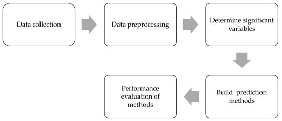
Figure 1.
Phases of the prediction process.
3.2. Data Collection
In this research, the monthly data on the economic indicators of inflation, minimum wage, gross domestic product (GDP), gross fixed capital formation (GFCF), and unemployment rate in Ecuador from January 2002 to December 2019 were prepared by the Central Bank of Ecuador (BCE), the National Institute of Statistics and Censuses (INEC), and the Ministry of Labor of Ecuador; part of this data is available on official websites, while others were provided by the aforementioned organizations for the purposes of unifying the information that was required in this investigation. The figures for inflation, GDP, and GFCF were obtained from the Central Bank of Ecuador, the minimum wage from the Ministry of Labor of Ecuador, and the unemployment rate from the National Institute of Statistics and Censuses of Ecuador (INEC).
The features of inflation, minimum wage, GDP, and GFCF were selected from official sources in order to guarantee the coherence and reliability of the analyses. This choice is based on its close relationship with the unemployment rate. These indicators have proven to be of great relevance since they exert direct or indirect influence on the dynamics of the labor market, with a significant impact on unemployment trends.
3.3. Data Preprocessing
The necessary preprocessing techniques that were applied to ensure the quality of the data were the analysis to check the existence of outliers and the need to treat them, the matching of the range of observations in the data set, and the normalization of the input values (X). These techniques are described below:
The process of preparing the data for subsequent detailed analysis consisted of performing data cleaning by removing missing observations from the data set. In this sense, the five indicators obtained were the inflation rate, the minimum wage, GDP, GFCF, and the unemployment rate; the GDP and the GFCF had a range of data from 2000 to 2020 and the inflation rate, minimum wage, and unemployment rate from 2002 to 2020, so it was decided to match the range of years and omit the year 2020 to correspond to the time of the COVID-19 coronavirus pandemic and be considered valid outliers. Likewise, the minimum wage was deflated based on 2007. No missing values were found in the data set.
To determine outliers in characteristics, the interquartile range (IQR) technique was used using the 1.5 IQR rule, which designates any value greater than and any value less than as an outlier (Table 2).
Table 2.
Determining outliers in features.
The unemployment rate is an economic indicator that refers to the portion of people who are actively looking for work but cannot find work. This measure of the prevalence of unemployment can be a good indication of the economic situation of the country [24]. A low unemployment rate is generally a sign of a good economy. The data set has 216 observations, four input variables, and the unemployment rate, which is the output variable (target). There is no defined way to divide the data into training, validation, and testing. In the literature, most researchers have suggested splitting the data as 60:20:10, 70:20:10, or 80:10:10 [25]. Therefore, we have divided the data set as follows: for the GA-LSTM prediction model, 80% of the data is for training, 10% for validation, and 10% for testing purposes; for the rest of the prediction models, 90% of the data is for training and 10% for testing purposes. This division allows us to predict the last 22 months of the unemployment rate using the individual algorithms (BiLSTM and GRU) and the last 19 months of this economic indicator using the hybrid GA-LSTM algorithm due to the sliding length of the temporal sequence of data (window size of 3). Before training the proposed models, the input data were standardized using the StandardScaler class of Scikit-learn’s preprocessing module, where the mean is removed and the data are scaled to unit variance, as follows:
where indicates the normalized value, represents the actual value, is the mean of the training samples or zero, and is the standard deviation of the training samples or one.
3.4. Determine Significant Variables
The unemployment rate is affected by many factors. Therefore, it is necessary to consider all these economic indicators in the prediction system, such as GDP, value added of primary, secondary, and tertiary industries, consumer price index (CPI), investment in fixed assets, total imports and exports, total retail sales of consumer goods, financial expenses, number of urban residents, disposable income of urban residents, balance of savings deposits of urban and rural residents, the value aggregate of the entire industry of the city, population number, inflation rate, and average gross monthly salary [17,26,27]. Based on the relevant research, 4 factors have been selected as indicators of the prediction model: the inflation rate, the national minimum wage, the GDP, and the GFCF.
The Pearson correlation coefficient was used to measure the relationship between the predictor variables and the target variable (Table 3). It is calculated as the covariance between two characteristics, x and y, divided by the product of their standard deviations.
Table 3.
Significant variables.
The monthly view revealed a statistically significant linear relationship between the minimum wage and the unemployment rate, GDP and the unemployment rate, and the GFCF and the unemployment rate (with a negative relationship). The inflation rate shown here is not correlated with the characteristics of the unemployment market (Figure 2).
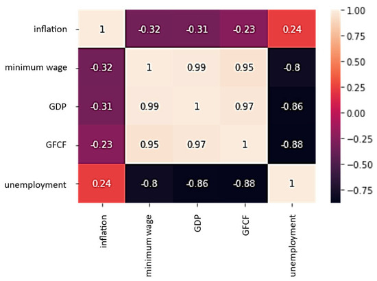
Figure 2.
Heat map of unemployment rate vs. inflation, minimum wage, GDP, and GFCF.
Based on the above tests, the final columns selected for machine learning are minimum wage, GDP, and GFCF, and the target column is the unemployment rate.
3.5. Build Prediction Methods
The BiLSTM, GRU, and GA-LSTM prediction methods used in this study are briefly described below.
3.5.1. Bidirectional LSTM (BiLSTM)
A BiLSTM is a type of recurrent neural network where the signal is propagated backward and forward in time, i.e., it allows additional training by traversing the input data twice: from left to right and from right to left [28]. BiLSTM has demonstrated good results in many fields, such as natural language processing, semantic segmentation of the QRS complex, prediction or forecasting of time series, and phoneme classification, among others.
As the output sequence of the forward LSTM layer is commonly obtained as the unidirectional one, the output sequence of the reverse LSTM layer is calculated using the reverse inputs from time to time . These output sequences are then fed to the function to combine them into an output vector [29]. Similar to the LSTM layer, the final output of a BiLSTM layer can be represented by a vector, , in which the last element, , is the estimated unemployment rate for the next iteration.
3.5.2. Gated Recurrent Unit (GRU)
The GRU are similar to the LSTM; they were created to solve the vanishing gradient problem; for this, they use two gates (restart and update) instead of the three gates that LSTM uses. The reset gate is used to determine how much information from the past is forgotten, and the update gate decides what information to discard and what new information to add. In the GRU structure, the reset gate selects information from the previous state to be discarded, and the update gate selects new information from the input vector and the previous state to be added to a new state. The candidate for the future hidden state is found by the candidate state gate [30]. Compared with an LSTM-based model, a GRU-based model has a simpler structure and fewer tensor operations (about 25% less) due to the fusion of the cell state and the hidden state, making it easier to train the model and making it a very suitable candidate for integrated implementations [31].
3.5.3. A Hybrid Intelligence of LSTM and the Genetic Algorithm (GA)
Evolutionary algorithms (EA) are stochastic search and optimization methods that are based on genetic inheritance and ideas from Darwinian evolution. The paradigms of evolutionary computing are evolutionary programming, evolutionary strategies, and genetic algorithms. In this sense, genetic algorithms are optimization methods used to solve nonlinear, non-differentiable, discontinuous, or multimodal optimization problems. These algorithms are applied to solve optimization, classification, and regression problems [32]. Its operation generally consists of starting with an initial generation of candidate solutions, randomly generated or another method, which is tested with the objective function; then the following generations are produced, which evolve from the first generation through the typical genetic operators of selection, crossing, and mutation. Chromosomes, which represent a better solution to the objective problem, have a few more opportunities to “reproduce” and “survive” than those chromosomes that have poorer and “weaker” solutions. The “goodness” of a solution is usually defined with respect to the current population [33].
Evolutionary algorithms have been widely applied to neural networks, and various hybrid approaches have also been used for economic time series prediction. Genetic algorithms allow the learning algorithm to be improved by acting as a network training method, feature subset selection, and neural network topology optimization, as well as reducing the complexity of the feature space [34].
Figure 3 shows the hybrid GA-LSTM approach to find the time window size and the number of LSTM units for the prediction of the unemployment rate in Ecuador. Determining the time window and the number of LSTM units is quite important for the performance of the algorithm. If the window size is too small, the model will neglect important information, or if it is too large, the model will overfit the training data.
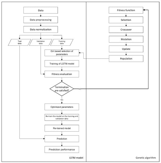
Figure 3.
Procedure of the GA-LSTM hybrid model for the prediction of the unemployment rate.
Initially, the study consisted of designing the appropriate network parameters for the LSTM network. We use an LSTM network to solve the prediction problem using the feedforward architecture. This architecture consists of a sequential input layer, a Keras LSTM layer, and a dense output layer. GA investigates the optimal number of hidden neurons in the LSTM layer. In the GA-LSTM model, the hyperbolic tangent function is used as an activation function for the input nodes and the LSTM nodes, while the linear function is used as an activation function at the output node. The hyperbolic tangent function is a scaled sigmoid function and returns the input value in a range between −1 and 1, and the linear activation function (identity) is directly proportional to the input, allowing the output to vary continuously and linearly. The activation function of the output node is designated as a linear function because our goal is the prediction of next month’s unemployment rate, which can be formulated as a regression problem. The initial network weights are set as random values, and the network weight is adjusted using the “Adam” stochastic optimization method; this optimization algorithm was developed by Kingma and Ba. Among its characteristics, it stands out that it is simple to implement, it is computationally efficient, it has few memory requirements, it is suitable for problems that are large in terms of data and/or parameters, and it is appropriate for non-stationary objectives, among others [35].
We then employ the GA heuristic search method to investigate the optimal size of the time windows and the architectural factors of the LSTM network. Various time window sizes and different numbers of units are applied in the LSTM layer to evaluate the fitness of GA. Populations are composed of possible solutions and are initialized with random values before genetic operators start exploring the search space. The chromosomes used in this study are encoded in binary bits that represent the size of the time window and the number of LSTM units; specifically, each chromosome is represented by nine bits, of which five bits are for the window size and four bits for the number of units. Once the population is initialized, the crossover operations are used for pairing, mutation to rearrange the chromosomes, and the roulette selection algorithm to select the parents and find the superior solution. Solutions are evaluated using a predefined fitness function, and the best-performing chromosomes are selected for breeding. The fitness function evaluates how close a given solution is to the optimal solution of the desired problem. This function is a crucial part of the GA, so it has been chosen carefully. In this research, we use RMSE to calculate the fitness of each chromosome, and the subset of architectural factors that produced the smallest RMSE is selected as the optimal solution. If the output of the breeding process satisfies the termination criteria, the derived optimal or near-optimal solution is applied to the predictive model. Otherwise, the selection, crossover, and mutation processes of the genetic algorithm are repeated. To acquire a superior solution for the problem, genetic parameters such as crossover rate, mutation rate, and population size can affect the outcome. Previous research has suggested setting genetic algorithm parameters to specific values, such as a population of (4, 10, 20), a crossover probability of (0.7, 0.4, 0.6), and a mutation probability of (0.15, 0.1, 0.3) [36,37,38]. There is no established consensus on the optimal population size, and crossover and mutation values are generally in the range of 0 to 1. These studies have provided an initial basis for setting up and evaluating various combinations of genetic algorithm values, thus seeking to find the optimal configuration of model parameters that allows for improving the predictive performance of the test data. In this study, we have adopted an approach based on the above findings by setting a population size of 4, a crossover rate of 0.6, and a mutation rate of 0.4 in the experiment. As a stopping condition, the number of generations is assigned to 10.
To determine if the LSTM network architecture is suitable for prediction, several experiments were performed, varying the hyperparameters and evaluating the performance of the model. This involved building and training multiple LSTM models with different configurations, evaluating their performance using the RMSE metric, and selecting the best-performing model. This iterative approach allows us to identify the optimal combination of hyperparameters that maximizes the predictive capacity of the model for a specific task. Using this systematic approach, we use an LSTM network with a sequential input layer followed by an LSTM hidden layer and a dense output layer, and GA investigates the optimal number of neurons in each hidden layer. Subsequently, the parameter optimization process in the GA-LSTM model was carried out rigorously to improve the predictive ability of the unemployment prediction task. We started by importing a variety of essential libraries and modules to manipulate data, design the LSTM neural network, and run the genetic algorithm. Furthermore, we imported the unemployment time series data in CSV format and prepared it by dividing it into sequences of specific length to be used as input for the LSTM network. We define a training and evaluation function that creates and trains the LSTM network for each individual of the genetic algorithm, using the RMSE metric to evaluate the training accuracy on a validation set. The structure of the genetic algorithm was defined with the DEAP library, specifying characteristics such as gene size, population, crossover, mutation, and selection operations. We run the genetic algorithm to evolve the population and select the best individual from the last generation as the best solution. These optimal parameters, such as the window size and the number of units of the LSTM network, were used to build and train the neural network. The choice of these parameters was based on the need to maximize the performance of the model and improve its ability to capture complex patterns in unemployment time series data.
Integrating an LSTM neural network with a GA involves combining the learning capability of the neural network to model sequential data with the optimization capability of the genetic algorithm to search for the best set of hyperparameters for the neural network. The specific steps involved in this process are detailed below:
- Import the libraries and modules necessary for prediction. This includes libraries for manipulating data (NumPy, Pandas, and Scikit-learn), plotting data (Matplotlib), neural networks (Keras), and genetic algorithms (DEAP), as well as extra libraries for manipulating bit structures (Bitstring) and generating random binary values using the Bernoulli distribution (SciPy).
- Import the time series data; the time series will be used for model training and evaluation. The unemployment data are expressed in a comma-separated value (CSV) format.
- Prepare the data set; the data are divided into sequences of specified length (window size), which will be used as input for the LSTM neural network. In addition, the corresponding input and output data are prepared.
- Define the training and evaluation function “train_evaluate” that creates and trains the LSTM neural network for a given individual of the genetic algorithm. This function returns the training accuracy using the RMSE metric on a validation set.
- Define the structure of the genetic algorithm; the DEAP library is used to define the structure of the genetic algorithm. Characteristics of individuals are defined, such as gene size, population, crossover, mutation and selection operations, and the fitness evaluation function of each individual in the population.
- Run the genetic algorithm to evolve the population over several generations. During each generation, individuals are crossed, mutated, and selected for fitness.
- Select the best individual from the last generation as the best solution found by the genetic algorithm. The optimal parameters of this individual are specified (number of windows and number of units of the LSTM model) by setting the values in the variables “window_size_bits” and “num_units_bits”.
- Use the best solution found to build and train the LSTM neural network with the optimal parameters. The model is trained using the training data set, and its performance is evaluated using the test data set. During training, the cross-validation technique is used, where 10% of the training data is reserved as a validation set. This process allows model performance to be monitored on unseen data while tuning hyperparameters to avoid overfitting and improve model generalization.
- Finally, the results obtained by the model are graphed. The model predictions are compared with the actual values of the time series.
The described process allows integrating an LSTM neural network with a genetic algorithm to optimize the hyperparameters of the model and improve its predictive capacity in the unemployment prediction task.
The Python code for our hybrid GA-LSTM prediction method is released on the GitHub repository “unemployment rate prediction” at https://github.com/kevinmero/Unemployment-rate-prediction (accessed on 19 February 2024).
3.6. Performance Evaluation of Methods
To evaluate the prediction performance of the GA-LSTM model before the BiLSTM and GRU reference approaches, the criteria described by Chung and Shin (2018) were used in our research, consisting of the mean square error (MSE), the mean absolute error (MAE), and the mean absolute percentage error (MAPE) [39]. These evaluation measures can be calculated as follows:
where residual error = ; is the actual output; is the predicted output; and is the number of predictions.
The paired t-test formula is as follows [40]:
where is the observed mean difference; is the standard error of the observed mean difference; and n is the number of differences.
The selection of the evaluation metrics MSE, MAE, and MAPE in unemployment prediction allows a comprehensive evaluation of the performance of the proposed model.
The MSE is used to calculate the means of the squared differences between the observed values and the predicted values, providing a measure of the spread of the squared errors and their average. On the other hand, the MAE is used to determine the mean of the absolute differences between the observed values and the predicted values, which is useful to evaluate the overall accuracy of the model in terms of absolute deviation. In addition, the MAPE is responsible for measuring the average percentage differences between the observed values and the predicted values. It is especially useful in tasks where sensitivity to relative variations is more important than sensitivity to absolute variations [41].
In general, even small discrepancies in the values of these metrics can influence decisions and actions taken in the economic and social spheres. It is vital to consider the limitations of these metrics: compared to MAE, MSE may be more affected by outliers due to its quadratic nature; MAE may not accurately reflect model performance if the data set used for testing contains many outlier values; and with respect to MAPE, its use is restricted to strictly positive data by definition, as well as its bias towards low forecasts, which makes it inappropriate for predictive models where large errors are expected [42].
4. Results
In this section, all algorithms are coded in Python (version 3.8.16). Our models were implemented using the Python Keras deep learning library (version 2.9.0) and the TensorFlow backend (version 2.9.2). Additionally, other major packages such as NumPy (version 1.21.6), Pandas (version 1.3.5), and Matplotlib (version 3.2.2) were used to process, manipulate, and visualize data; Deap (version 1.3.3) and Bitstring (version 4.0.1) were required in the LSTM-GA model as an evolutionary computing framework and for binary data management. All experiments were carried out on a personal computer with an Intel Core i7-8750H processor (Intel, Santa Clara, CA, USA), a 2.20 GHz CPU (×64), 16 GB of RAM, and the Windows 10 operating system. The hybrid algorithm processes 216 observations in an approximate runtime of around 5 min. The Google Collaboratory (Colab) cloud service is used, and the Anaconda platform, specifically the GA-LSTM algorithm, was made and executed on Google Colab. Stand-alone algorithms were built in Anaconda (version 2.3.2) due to usage limits and the availability of Colab hardware at no cost. Colab from Google Research is ideal for application in data science projects related to machine learning, deep learning, and data analysis. The main identified advantages of this product are that it requires no configuration, free access to computational resources (such as executing code in a GPU runtime environment), and easy sharing of online content. On the other hand, the Anaconda platform is used for scientific computing, such as data science and machine learning, and has thousands of scientific Python packages and libraries that facilitate the development and maintenance of the system [43].
The hyperparameter tuning of neural models is important because it optimizes the learning process [44]. Therefore, the corresponding parameter values significantly influence the performance of BiLSTM, GRU, and GA-LSTM. For the hybrid algorithm, the parameters are set as follows: the population is 4, the crossover probability is 0.6, the mutation probability is 0.4, and the number of generations is 10. Meanwhile, the parameters of LSTM are set as follows: the number of hidden layers is 1, the number of hidden units is 12, the window number is 3, the batch number is 10, and the number of epochs is 5.
In the case of the individual algorithms, combinations were tested using the GridSearchCV technique present in the Scikit-learn library: the number of hidden layers is (1, 2), the number of hidden units is (2, 3, 4, 5, 6, 7, 8), the batch number is (2, 4, 8, 10, 12, 14), the number of epochs is (32, 34, 36, 60, 65, 70, 75, 80), and the optimizers are (RMSprop, Adam).
In the experiments, we apply the hybrid GA-LSTM algorithm to the first 80% of the data as a training set, the next 10% of the data as a validation set, and the rest of the data set as test data. With respect to prediction evaluations, we have considered some of the indices used to evaluate the performance of the algorithms in the experiments, specifically the MSE, MAE, and MAPE indices, as well as the paired t-test.
This study applies a genetic algorithm to examine the optimal architectural parameters, window size, and units that feed the LSTM neural network, obtaining results through a genetic search. The best time window size for unemployment rate prediction chosen by GA has been 3; in other words, it is more effective to analyze the unemployment rate using information from the last three months of unemployment to predict the unemployment rate. Furthermore, the optimal number of LSTM units obtained that constitute the hidden layer has been 12 units.
We trained the hybrid model with the best parameters, applied the input embedding of the last three-time steps, and optimized the architecture to verify the effectiveness of the GA-LSTM model on the holdout data. The result derived from the GA-optimized LSTM network is measured by calculating the three mentioned performance indices of the actual unemployment rate and the output of the proposed hybrid model.
The results of BiLSTM, GRU, and GA-LSTM are presented below in Table 4. It should be noted that we chose the best results of the individual algorithms by testing various combinations, as previously discussed.
Table 4.
The performance measure of models for predicting the unemployment rate.
According to the data presented in Table 5, the MSE, MAE, and MAPE metrics were used following the reference of Chung and Shin (2018); in this sense, they must be interpreted as follows:
Table 5.
Performance of metrics.
The smaller the MSE, MAE, and MAPE values, the better the prediction effect of the model.
The results reveal quantitative data that allows us to obtain the following findings:
- (a)
- As shown in Table 4, machine learning models can establish unemployment prediction models with reasonable results according to MAPE values. However, GA-LSTM performs better than BiLSTM and GRU. For MSE, the best result of GA-LSTM is 0.052, while the results of BiLSTM and GRU are 0.130 and 0.072, respectively. Meanwhile, for MAE, the best result of GA-LSTM is 0.200, while for BiLSTM and GRU, the best results are 0.291 and 0.220, respectively. For MAPE, GA-LSTM is also better. Furthermore, when the NHL is 2, the results are always better in the GRU model compared to BiLSTM.
- (b)
- The performance of GA-LSTM is better in MSE, MAE, and MAPE metrics; GRU, with two hidden layers, is the next model that presents the best predicted results.
- (c)
- The features selected in the study for GA-LSTM and the individual BiLSTM and GRU models achieved a good result.
- (d)
- The proposed GA-LSTM works well with the configurations (1, 12, 3) for the number of hidden layers, units, and windows, respectively.
Additionally, the data were analyzed using the paired t-test formula. The paired t-test is a proper statistical technique to determine whether the mean of the differences between two paired contexts (two prediction models) is different from 0. The hypothesis to be tested is that the paired predictive models do not have identical performance. The statistical significance of the test is determined by looking at the p-value. The hypothesis would be validated with p-values close to zero for the paired predictive models, while values close to 1 would invalidate the hypothesis. A 1% significance level was used to validate the proposed hypothesis using a t-test (p-value ≤ 0.01).
The results of the t-test validate the hypothesis for most of the proposed models, except in the cases of GA-LSTM (one layer) vs. GRU (two layers) and BiLSTM (one layer) vs. BiLSTM (two layers), where there is not enough evidence to conclude that there is a significant difference. Therefore, from a statistical point of view, the performance of these two proposed model case exceptions is very comparable.
Likewise, there is no statistically significant difference between the actual scores obtained from the scale and the scores obtained with the GA-LSTM (one layer) approach (t(18) = −2.81; p > 0.01). This result shows no difference between the unemployment rate scores estimated by GA-LSTM (one layer) and the actual scores. Therefore, the real scores and the artificial scores of GA-LSTM (one layer) are close, and the GA-LSTM 1L model predicts results close to the real unemployment rate scores. For comparative models, the real scores and the artificial scores are not close to each other.
Figure 4 shows the actual values and estimated values of the BiLSTM, GRU and GA-LSTM prediction models.
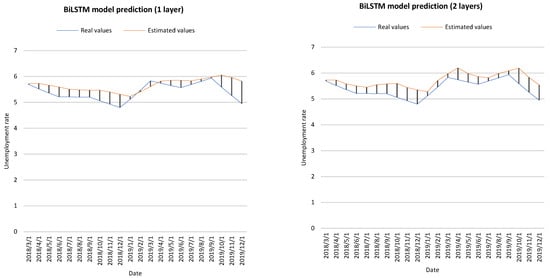
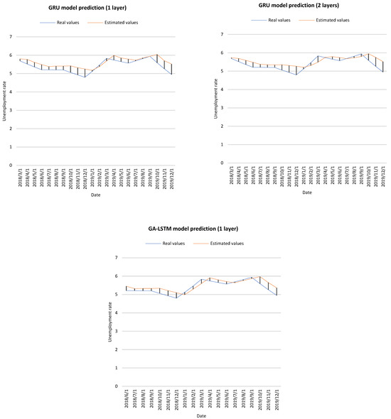
Figure 4.
Prediction results of different approaches.
5. Discussion
The above results show that the proposed GA-LSTM approach has performed well in predicting the unemployment rate in Ecuador. The approach’s advantages compared to the individual models in the study are that GA allows for the automatic finding of the best parameters (i.e., optimal combination) for the LSTM algorithm. Finding the optimal values in machine learning (ML) is a great challenge because the hyperparameters in the algorithms control various aspects of the training of the data. This task in past research has primarily depended on the expertise of the researchers; however, it should be considered that time and computational limitations make it impossible to sweep a parameter space to find the optimal set of input variables for an algorithm [39]. Furthermore, satisfactory results can be obtained with a small number of features (three in this study) and a limited sample.
The strengths and weaknesses of the models used in the study are shown below (Table 6).
Table 6.
Comparison of the BiLSTM, GRU, and GA-LSTM models.
The comparison table provides a clear view of the strengths and weaknesses of the three recurrent neural network models, i.e., BiLSTM, GRU, and GA-LSTM. It is observed that each model has distinctive characteristics that make it suitable for different contexts and applications. BiLSTM excels at capturing long-term dependencies in sequential data, while GRU offers a simpler architecture and faster training times, making it preferable in situations where computational efficiency is critical. On the other hand, the hybrid GA-LSTM approach combines the search space exploration capability of genetic algorithms with the long-term dependency capture capability of LSTM, resulting in superior performance in terms of prediction accuracy. Unemployment rate compared to the other two models. Despite its higher complexity and computational requirements, the GA-LSTM hybrid model shows a promising ability to improve the accuracy of unemployment rate prediction.
Regarding the limitations of this study, it is essential to highlight some assumptions and restrictions that could affect the generalization of the findings to other contexts. First, the research focused exclusively on predicting the unemployment rate in Ecuador, which could limit the applicability of the results to other countries or regions with different economic and social conditions. Furthermore, the data set’s small size could affect the trained models’ robustness, especially when considering additional variability factors that could influence the unemployment rate. Selected input characteristics, such as minimum wage, gross domestic product (GDP), and gross fixed capital formation (GFCF), may not fully capture the complexity of the factors influencing unemployment, which could limit the ability of the model to generalize to other contexts where different variables might be more relevant. Finally, although the GA-LSTM approach showed good results in this study, training on larger data sets could require considerable time due to its computational complexity. Consequently, it is recognized that generalization of the findings to other contexts should be done with caution, considering these limitations and the need to validate the model in different contexts before its practical implementation.
The selection of input data used in prediction systems is a critical issue. Inflation, minimum wage, GDP, and GFCF characteristics were selected from official sources to ensure consistency and reliability of the analyses. However, some possible limitations or biases in the data set are the variability in the availability of certain data (periods of missing data) and the fact that the selected economic indicators may not fully capture all the factors that influence unemployment trends.
6. Conclusions
The present work evaluated the accuracy of the hybrid GA-LSTM system and the deep learning neural networks BiLSTM and GRU to predict the unemployment rate in Ecuador. Three characteristics influencing the unemployment rate were considered and used to train the model. The proposed neural network models were based on three measures, MSE, MAE, and MAPE, to predict the unemployment rate. The predictions generated by the proposed models were calculated and compared with actual data; the GA-LSTM, BiLSTM, and GRU models demonstrated a high level of accuracy in capturing the various changes within the data set. However, because the differences are minor between the actual values and those predicted by the model, a paired t-test was required to make an informed decision. The results showed that the performance of the GA-LSTM models (one layer) vs. GRU (two layers) and BiLSTM (one layer) vs. BiLSTM (two layers) is very comparable. Likewise, the t-test allows testing whether the predictive accuracy of the prediction models differs significantly from the fundamental values of the unemployment rate. The hybrid GA-LSTM model (one layer) predicts results close to the actual unemployment rate scores. The predictions were calculated from the sample for 22 months based on the BiLSTM and GRU neural network models and 19 months in the case of the GA-LSTM hybrid model.
In terms of economic policy, the results can help anticipate future trends in the level of unemployment in the country. Thus, those responsible for economic and labor policy can have advanced information on the behavior of the labor market in the coming months and develop support programs for the unemployed. Likewise, with accurate predictions of the level of unemployment, governments can implement preventive measures against unemployment even before it occurs, either through the efficient allocation of public resources, incentives for the creation of new jobs, or the improvement of labor laws. That allows companies the possibility of increasing their labor supply.
Regarding the relevance of these results, their importance lies in their usefulness as inputs for carrying out more in-depth research on the labor market in general and unemployment in particular, since it is necessary to consider what factors can influence unemployment predictions and thus propose more effective economic policies. Finally, these results can raise awareness in society about the moments in which the level of unemployment can increase, and thus families would be better informed to adjust their budgets in the face of an imminent rise in the level of unemployment.
The importance of selecting an appropriate neural network architecture to evaluate the accuracy of unemployment prediction was fundamental, that is, deciding on the appropriate number of input nodes and hidden nodes, because it plays a vital role in evaluating the accuracy of neural network prediction. Different combinations of time window size and number of memory cell units can be tried to predict monthly unemployment performance. However, it requires a lot of time and experience on the part of researchers, so a genetic algorithm was adopted to optimize the hyperparameters of the hybrid model. Choosing a suitable neural network architecture is crucial when building unemployment rate prediction models, so one should be careful when choosing an unemployment rate prediction model.
One of the main limitations of our study lies in the inherent complexity of the labor market in Ecuador since there have been abrupt changes in the unemployment environment. Moreover, there is no open data with detailed information on the local unemployment rate provided by official institutions. Therefore, we had to do a PDF transcript of the economic reports, including the pandemic period.
It is important to note that while unemployment prediction is valuable in anticipating economic trends, policymakers must also understand the underlying causes of unemployment and develop strategies to address it effectively. Therefore, future research should focus on further analyzing the factors that influence labor market dynamics in Ecuador and how policies can mitigate unemployment and promote labor inclusion.
Although unemployment prediction models can be valuable tools for policymakers and researchers, it is crucial to recognize their limitations and complement the analysis with a broader focus on understanding the causes and consequences of unemployment in Ecuador. Future research should consider not only improving prediction accuracy but also developing more effective strategies to address unemployment and promote job stability in the country. It is also intended to investigate the application of GA-LSTM modeling compared to other hybrid models for predicting economic indicators in several data sets from other countries.
Another possible extension of the work is to explore other hybrid model architectures such as ARIMA-ARNN, ARIMA-LSTM, ARIMA-GRU, ARMAX-GARCHX, ARIMA-SVM, and ARIMA-LR, among others, in the prediction of economic indicators. Furthermore, applying the GA-LSTM methodology to a broader range of economic indicators, such as GDP, consumer price index, producer price index, exchange rate, stock market, energy consumption, house price, construction cost index, employment rate, and inflation, is crucial. This diversified approach would allow for a comprehensive evaluation of the effectiveness of the GA-LSTM model in predicting a variety of key economic indicators, from economic growth to consumer confidence and public debt. Expanding the scope of the methodology would provide us with a more complete and accurate view of the economic landscape, which is essential to addressing current and future economic challenges.
Author Contributions
Conceptualization, N.S. and J.P.-D.; methodology, K.M., J.M. and S.V.; software, K.M.; validation, J.M. and S.V.; formal analysis, K.M., J.M. and S.V. investigation, K.M., N.S., J.M. and S.V.; resources, J.P.-D.; data curation, K.M. and J.P.-D.; writing—original draft preparation, K.M.; writing—review and editing, K.M., N.S., J.M. and S.V.; visualization, J.M. and S.V.; supervision, J.M. and S.V. All authors have read and agreed to the published version of the manuscript.
Funding
The research has received funding from the Universidad Técnica de Manabí and Pontificia Universidad Católica del Ecuador.
Institutional Review Board Statement
Not applicable.
Informed Consent Statement
Not applicable.
Data Availability Statement
The data presented in this study are openly available from GitHub at the following link: https://github.com/kevinmero/Unemployment-rate-prediction/tree/main/data (accessed on 19 February 2024).
Conflicts of Interest
The authors declare no conflicts of interest.
Abbreviations
| RNN | Recurrent neural networks |
| LSTM | Long short-term memory |
| GA | Genetic algorithm |
| GA-LSTM | GA with long short-term memory |
| BiLSTM | Bidirectional LSTM |
| GRU | Gated recurrent units |
| GI | Google index |
| NN | Neural network |
| SVR | Support vector regressions |
| EU-LFS | European Union Labor Force Survey |
| SARIMA | Seasonal autoregressive integrated moving average |
| SETAR | Self-exciting threshold autoregressive |
| ETS | Error, trend, seasonal |
| NNAR | Neural network autoregression |
| RMSE | Root mean squared error |
| MAE | Mean absolute error |
| MAPE | Mean absolute percentage error |
| BMA-PAR | Bayesian model averaging with periodic autoregressive |
| SARMA | Seasonal autoregressive moving average |
| PMEANS | Seasonal (or periodic) MEANS |
| BPAR | Bayesian PAR |
| VAR | Vector autoregressive |
| SVAR | Spatial VAR |
| NN | Neural network |
| NNS | Neural network seasonal |
| SpVAR | Spatial vector autoregressions |
| SpNN | Spatial neural network |
| SpANN | Spatial artificial neural network |
| FARIMA | Fractional autoregressive integrated moving Average |
| FARIMA-GARCH | FARIMA with generalized autoregressive conditional heteroskedasticity |
| ANN | Artificial neural network |
| SVM | Support vector machine |
| MARS | Multivariate adaptive regression splines |
| ARMA | Autoregressive moving average |
| BIC | Bayesian information criterion |
| FTS | Fuzzy time series |
| NMSE | Normalized mean square error |
| ARIMA | Autoregressive integrated moving average |
| ARNN | Autoregressive neural network |
| ARIMA-SVM | ARIMA with support vector machine |
| ARIMA-ANN | ARIMA with artificial neural network |
| ARIMA-ARNN | ARIMA with autoregressive neural network |
| PSO | Particle swarm optimization |
| ARMAX-GARCHX | Stochastic linear autoregressive moving average with exogenous variable with GARCHX |
| GARCH | Generalized autoregressive conditional heteroskedasticity |
| GARCHX | Generalized autoregressive conditional heteroscedasticity with exogenous variable |
| AIC | Akaike information criterion |
| HQ | Hannan and Quinn |
| ARMAX-GARCH | Stochastic linear autoregressive moving average with exogenous variable with GARCH |
| ACF | Autocorrelation Function |
| PACF | Partial autocorrelation function |
| LSTM-GRU | Long short-term memory with gated recurrent unit |
| GAs | Genetic algorithms |
| MSE | Mean squared error |
| GDP | Gross domestic product |
| GFCF | Gross fixed capital formation |
| IQR | Interquartile range |
| CPI | Consumer price index |
| EA | Evolutionary algorithms |
| ML | Machine learning |
References
- Li, Z.; Xu, W.; Zhang, L.; Lau, R.Y.K. An Ontology-Based Web Mining Method for Unemployment Rate Prediction. Decis. Support Syst. 2014, 66, 114–122. [Google Scholar] [CrossRef]
- Chakraborty, T.; Chakraborty, A.K.; Biswas, M.; Banerjee, S.; Bhattacharya, S. Unemployment Rate Forecasting: A Hybrid Approach. Comput. Econ. 2021, 57, 183–201. [Google Scholar] [CrossRef]
- Davidescu, A.A.; Apostu, S.-A.; Paul, A. Comparative Analysis of Different Univariate Forecasting Methods in Modelling and Predicting the Romanian Unemployment Rate for the Period 2021–2022. Entropy 2021, 23, 325. [Google Scholar] [CrossRef] [PubMed]
- Deng, W.; Wang, G.; Zhang, X.; Xu, J.; Li, G. A Multi-Granularity Combined Prediction Model Based on Fuzzy Trend Forecasting and Particle Swarm Techniques. Neurocomputing 2016, 173, 1671–1682. [Google Scholar] [CrossRef]
- Katris, C. Prediction of Unemployment Rates with Time Series and Machine Learning Techniques. Comput. Econ. 2020, 55, 673–706. [Google Scholar] [CrossRef]
- Bokanyi, E.; Labszki, Z.; Vattay, G. Prediction of Employment and Unemployment Rates from Twitter Daily Rhythms in the US. Epj Data Sci. 2017, 6, 14. [Google Scholar] [CrossRef]
- Ryu, P.-M. Predicting the Unemployment Rate Using Social Media Analysis. J. Inf. Process. Syst. 2018, 14, 904–915. [Google Scholar] [CrossRef]
- Vicente, M.R.; López-Menéndez, A.J.; Pérez, R. Forecasting Unemployment with Internet Search Data: Does It Help to Improve Predictions When Job Destruction Is Skyrocketing? Technol. Forecast. Soc. Chang. 2015, 92, 132–139. [Google Scholar] [CrossRef]
- Pavlicek, J.; Kristoufek, L. Nowcasting Unemployment Rates with Google Searches: Evidence from the Visegrad Group Countries. PLoS ONE 2015, 10, e0127084. [Google Scholar] [CrossRef]
- D’Amuri, F.; Marcucci, J. The Predictive Power of Google Searches in Forecasting US Unemployment. Int. J. Forecast. 2017, 33, 801–816. [Google Scholar] [CrossRef]
- Xu, W.; Li, Z.; Cheng, C.; Zheng, T. Data Mining for Unemployment Rate Prediction Using Search Engine Query Data. Serv. Oriented Comput. Appl. 2013, 7, 33–42. [Google Scholar] [CrossRef]
- Smith, P. Google’s MIDAS Touch: Predicting UK Unemployment with Internet Search Data. J. Forecast. 2016, 35, 263–284. [Google Scholar] [CrossRef]
- Mihaela, S. Improving Unemployment Rate Forecasts at Regional Level in Romania Using Google Trends. Technol. Forecast. Soc. Chang. 2020, 155, 120026. [Google Scholar] [CrossRef]
- Dilmaghani, M. Workopolis or The Pirate Bay: What Does Google Trends Say about the Unemployment Rate? J. Econ. Stud. 2019, 46, 422–445. [Google Scholar] [CrossRef]
- Vosseler, A.; Weber, E. Forecasting Seasonal Time Series Data: A Bayesian Model Averaging Approach. Comput. Stat. 2018, 33, 1733–1765. [Google Scholar] [CrossRef]
- Wozniak, M. Forecasting the Unemployment Rate over Districts with the Use of Distinct Methods. Stud. Nonlinear Dyn. Econom. 2020, 24, 20160115. [Google Scholar] [CrossRef]
- Ramli, N.; Ab Mutalib, S.M.; Mohamad, D. Fuzzy Time Series Forecasting Model with Natural Partitioning Length Approach for Predicting the Unemployment Rate under Different Degree of Confidence. In Proceedings of the 24th National Symposium on Mathematical Sciences (sksm24): Mathematical Sciences Exploration for the Universal Preservation; Salleh, Z., Hasni, R., Rudrusamy, G., Lola, M.S., Salleh, H., Rahim, H.A., AbdJalil, M., Eds.; American Institute of Physics: Melville, NY, USA, 2017; Volume 1870, p. 040026. [Google Scholar]
- Olmedo, E. Forecasting Spanish Unemployment Using Near Neighbour and Neural Net Techniques. Comput. Econ. 2014, 43, 183–197. [Google Scholar] [CrossRef]
- Ahmmed Mohammed, F. Applying Hybrid Time Series Models for Modeling Bivariate Time Series Data with Different Distributions for Forecasting Unemployment Rate in the USA. J. Mech. Contin. Math. Sci. 2019, 14. [Google Scholar] [CrossRef]
- Shi, L.; Khan, Y.A.; Tian, M.-W. COVID-19 Pandemic and Unemployment Rate Prediction for Developing Countries of Asia: A Hybrid Approach. PLoS ONE 2022, 17, e0275422. [Google Scholar] [CrossRef]
- Yurtsever, M. Unemployment Rate Forecasting: LSTM-GRU Hybrid Approach. J. Labour Mark. Res. 2023, 57, 18. [Google Scholar] [CrossRef]
- Ahmad, M.; Khan, Y.A.; Jiang, C.; Kazmi, S.J.H.; Abbas, S.Z. The Impact of COVID-19 on Unemployment Rate: An Intelligent Based Unemployment Rate Prediction in Selected Countries of Europe. Int. J. Financ. Econ. 2023, 28, 528–543. [Google Scholar] [CrossRef]
- Katoch, S.; Chauhan, S.S.; Kumar, V. A Review on Genetic Algorithm: Past, Present, and Future. Multimed. Tools Appl. 2021, 80, 8091–8126. [Google Scholar] [CrossRef] [PubMed]
- Tatarczak, A.; Boichuk, O. The Multivariate Techniques in Evaluation of Unemployment Analysis of Polish Regions. Oeconomia Copernic. 2018, 9, 361–380. [Google Scholar] [CrossRef]
- Zou, H.F.; Xia, G.P.; Yang, F.T.; Wang, H.Y. An Investigation and Comparison of Artificial Neural Network and Time Series Models for Chinese Food Grain Price Forecasting. Neurocomputing 2007, 70, 2913–2923. [Google Scholar] [CrossRef]
- Cheng, Y.; Hai, T.; Zheng, Y.; Li, B. Prediction Model of the Unemployment Rate for Nanyang in Henan Province Based on BP Neural Network. In Proceedings of the 13th International Conference on Natural Computation, Fuzzy Systems and Knowledge Discovery (icnc-Fskd); Liu, Y., Zhao, L., Cai, G., Xiao, G., Li, K.L., Wang, L., Eds.; IEEE: New York, NY, USA, 2017; pp. 1023–1027. [Google Scholar]
- Miskolczi, M.; Langhamrova, J.; Fiala, T. Unemployment and Gdp. In Proceedings of the International Days of Statistics and Economics; Loster, T., Pavelka, T., Eds.; Melandrium: Slany, Czech Republic, 2011; pp. 407–415. [Google Scholar]
- Siami-Namini, S.; Tavakoli, N.; Namin, A.S. The Performance of LSTM and BiLSTM in Forecasting Time Series. In Proceedings of the 2019 IEEE International Conference on Big Data (Big Data), Los Angeles, CA, USA, 9–12 December 2019; pp. 3285–3292. [Google Scholar]
- Cui, Z.; Ke, R.; Pu, Z.; Wang, Y. Deep Bidirectional and Unidirectional LSTM Recurrent Neural Network for Network-Wide Traffic Speed Prediction. arXiv 2019, arXiv:1801.02143v2. [Google Scholar] [CrossRef]
- Zarzycki, K.; Ławryńczuk, M. Advanced Predictive Control for GRU and LSTM Networks. Inf. Sci. 2022, 616, 229–254. [Google Scholar] [CrossRef]
- Rouhi Ardeshiri, R.; Ma, C. Multivariate Gated Recurrent Unit for Battery Remaining Useful Life Prediction: A Deep Learning Approach. Int. J. Energy Res. 2021, 45, 16633–16648. [Google Scholar] [CrossRef]
- Lugo Reyes, S.O. Chapter 21—Artificial Intelligence in Precision Health: Systems in Practice. In Artificial Intelligence in Precision Health; Barh, D., Ed.; Academic Press: Cambridge, MA, USA, 2020; pp. 499–519. ISBN 978-0-12-817133-2. [Google Scholar]
- Whitley, D. A Genetic Algorithm Tutorial. Stat. Comput. 1994, 4, 65–85. [Google Scholar] [CrossRef]
- Kim, K.; Han, I. Genetic Algorithms Approach to Feature Discretization in Artificial Neural Networks for the Prediction of Stock Price Index. Expert Syst. Appl. 2000, 19, 125–132. [Google Scholar] [CrossRef]
- Kingma, D.P.; Ba, J. Adam: A Method for Stochastic Optimization. arXiv 2017, arXiv:1412.6980. [Google Scholar] [CrossRef]
- Stajkowski, S.; Kumar, D.; Samui, P.; Bonakdari, H.; Gharabaghi, B. Genetic-Algorithm-Optimized Sequential Model for Water Temperature Prediction. Sustainability 2020, 12, 5374. [Google Scholar] [CrossRef]
- Thi Kieu Tran, T.; Lee, T.; Shin, J.-Y.; Kim, J.-S.; Kamruzzaman, M. Deep Learning-Based Maximum Temperature Forecasting Assisted with Meta-Learning for Hyperparameter Optimization. Atmosphere 2020, 11, 487. [Google Scholar] [CrossRef]
- Kara, A. Multi-Step Influenza Outbreak Forecasting Using Deep LSTM Network and Genetic Algorithm. Expert Syst. Appl. 2021, 180, 115153. [Google Scholar] [CrossRef]
- Chung, H.; Shin, K. Genetic Algorithm-Optimized Long Short-Term Memory Network for Stock Market Prediction. Sustainability 2018, 10, 3765. [Google Scholar] [CrossRef]
- Tello, R.; Crewson, P.E. Hypothesis Testing II: Means. Radiology 2003, 227, 1–4. [Google Scholar] [CrossRef] [PubMed]
- De Myttenaere, A.; Golden, B.; Le Grand, B.; Rossi, F. Mean Absolute Percentage Error for Regression Models. Neurocomputing 2016, 192, 38–48. [Google Scholar] [CrossRef]
- Chicco, D.; Warrens, M.J.; Jurman, G. The Coefficient of Determination R-Squared Is More Informative than SMAPE, MAE, MAPE, MSE and RMSE in Regression Analysis Evaluation. PeerJ Comput. Sci. 2021, 7, e623. [Google Scholar] [CrossRef] [PubMed]
- Alvarellos, A.; Figuero, A.; Sande, J.; Peña, E.; Rabuñal, J. Deep Learning Based Ship Movement Prediction System Architecture. In Proceedings of the Advances in Computational Intelligence; Rojas, I., Joya, G., Catala, A., Eds.; Springer International Publishing: Cham, Switzerland, 2019; pp. 844–855. [Google Scholar]
- Mateus, B.C.; Mendes, M.; Farinha, J.T.; Assis, R.; Cardoso, A.M. Comparing LSTM and GRU Models to Predict the Condition of a Pulp Paper Press. Energies 2021, 14, 6958. [Google Scholar] [CrossRef]
- Qazi, A.; Fayaz, H.; Wadi, A.; Raj, R.G.; Rahim, N.A.; Khan, W.A. The Artificial Neural Network for Solar Radiation Prediction and Designing Solar Systems: A Systematic Literature Review. J. Clean. Prod. 2015, 104, 1–12. [Google Scholar] [CrossRef]
- Pirani, M.; Thakkar, P.; Jivrani, P.; Bohara, M.H.; Garg, D. A Comparative Analysis of ARIMA, GRU, LSTM and BiLSTM on Financial Time Series Forecasting. In Proceedings of the IEEE International Conference on Distributed Computing and Electrical Circuits and Electronics (ICDCECE), Ballari, India, 23–24 April 2022; pp. 1–6. [Google Scholar]
- Shenfield, A.; Howarth, M. A Novel Deep Learning Model for the Detection and Identification of Rolling Element-Bearing Faults. Sensors 2020, 20, 5112. [Google Scholar] [CrossRef]


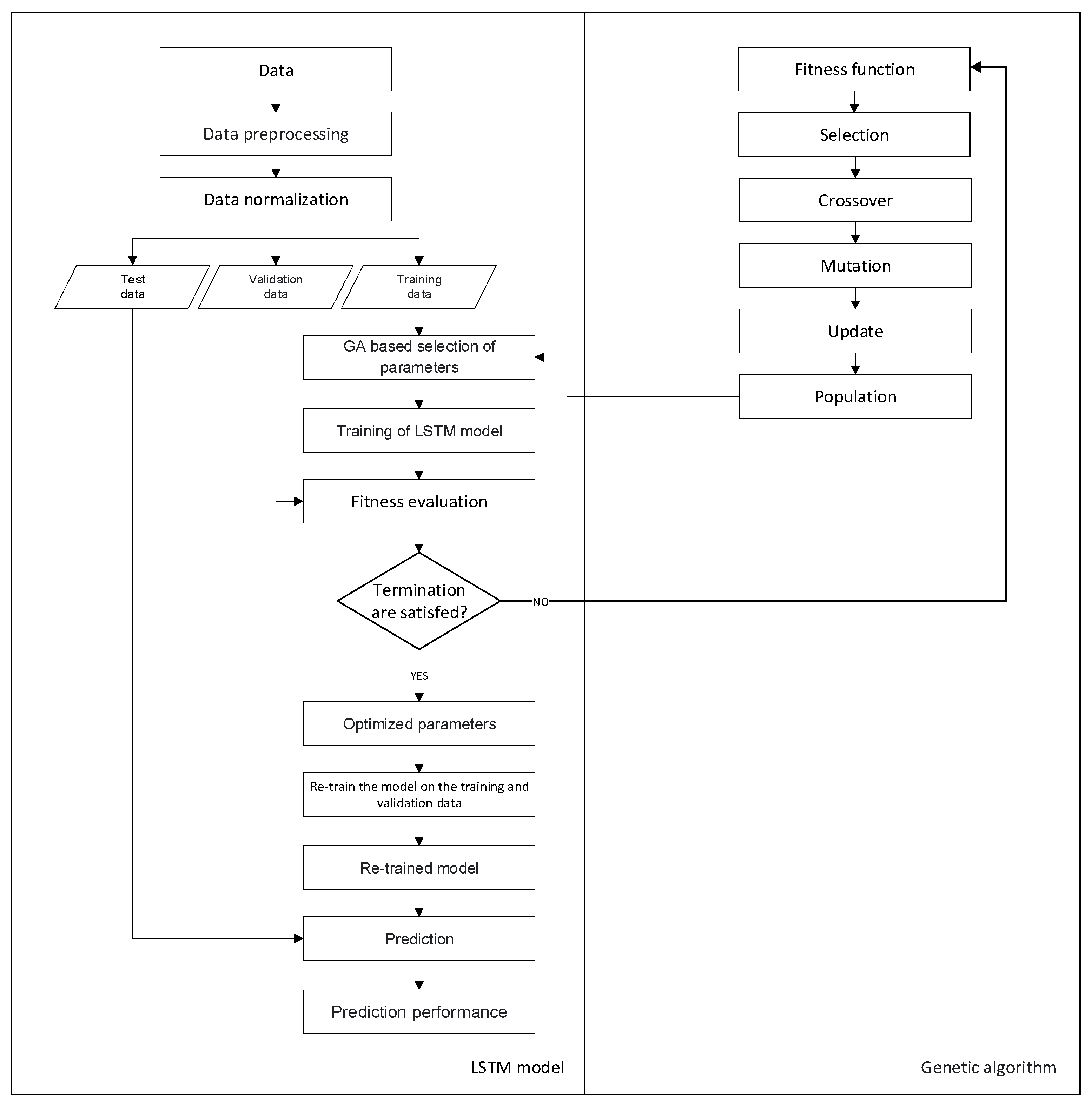
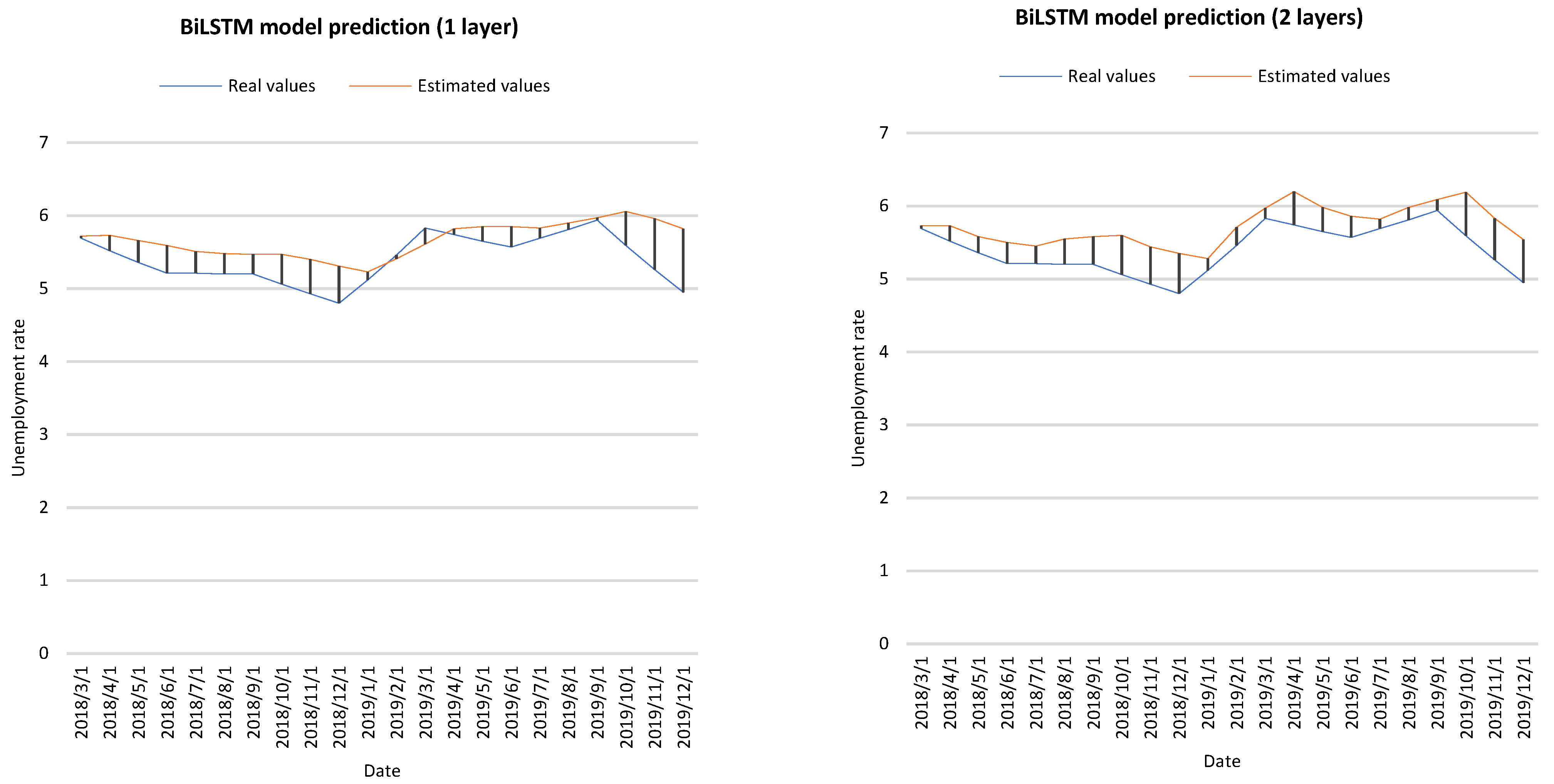
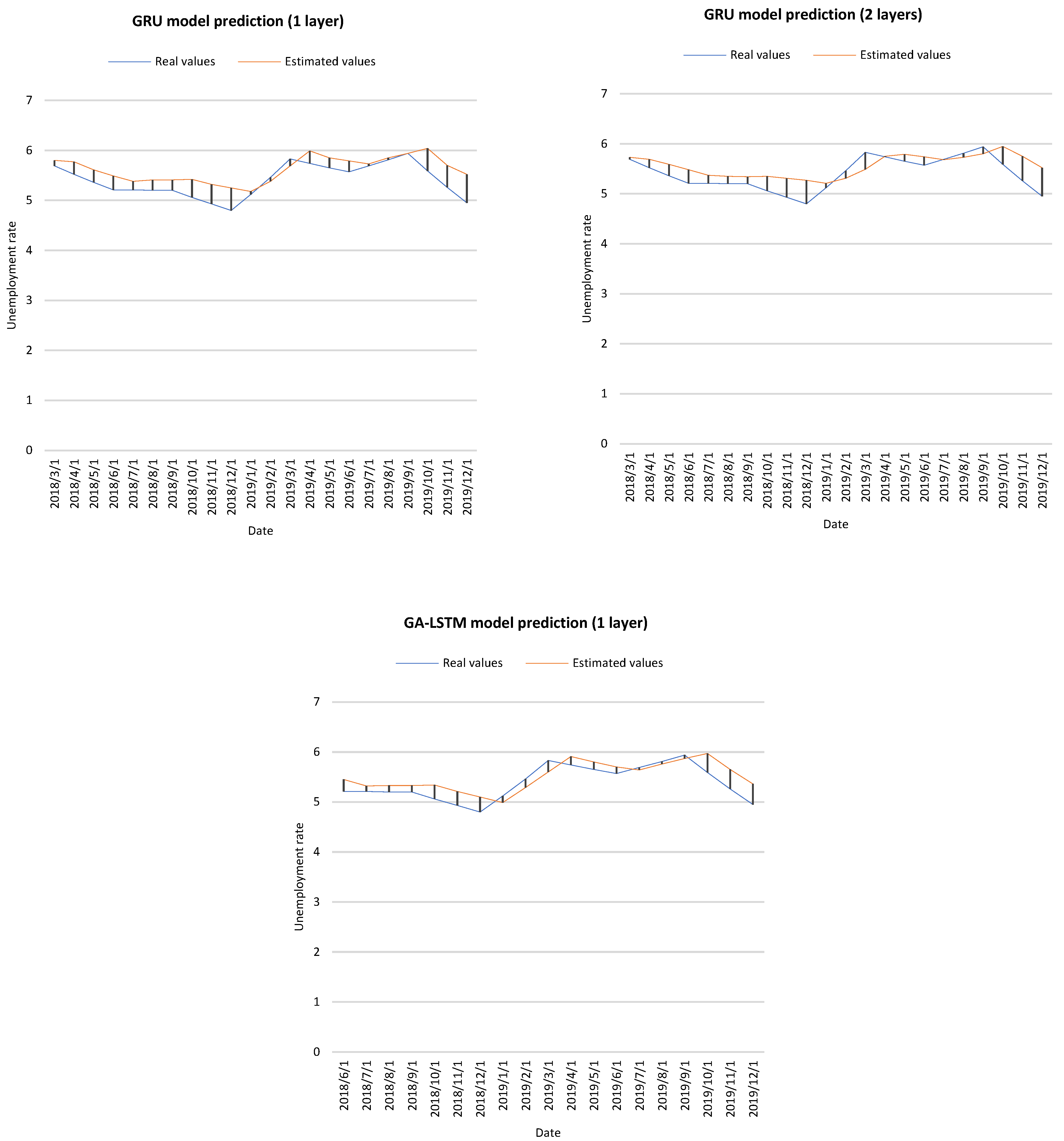
Disclaimer/Publisher’s Note: The statements, opinions and data contained in all publications are solely those of the individual author(s) and contributor(s) and not of MDPI and/or the editor(s). MDPI and/or the editor(s) disclaim responsibility for any injury to people or property resulting from any ideas, methods, instructions or products referred to in the content. |
© 2024 by the authors. Licensee MDPI, Basel, Switzerland. This article is an open access article distributed under the terms and conditions of the Creative Commons Attribution (CC BY) license (https://creativecommons.org/licenses/by/4.0/).