Predicting Rutting Development Using Machine Learning Methods Based on RIOCHTrack Data

Abstract

As the main cause of asphalt pavement distress, rutting severely affects pavement safety. Establishing an accurate rutting prediction model is crucial for asphalt pavement maintenance, pavement structure design, and pavement repair. This study explores five machine learning methods, namely Support Vector Regression (SVR), Artificial Neural Network (ANN), Gradient Boosting Decision Tree (GBDT), Random Forest (RF), and Extra Trees, to predict the development of rutting depth using data from RIOHTRack. The model’s performance is measured by comparing the performance evaluation indicators of different models, such as the coefficient of determination, root mean square error, mean absolute error, and mean absolute percentage error. The results demonstrate that integrated learning techniques such as RF, GBDT, and Extra Trees works best with R² = 0.9761, 0.9833, and 0.9747. Moreover, the GBFT model can capture the trend of the measured rutting progression curve better than the mechanistic-empirical (M-E) model. The analysis of feature importance reveals that, in addition to external factors such as temperature and axle load, the aggregate of the asphalt concrete layer and air void crucially affect rutting. The higher the base strength, the smaller the rutting depth. The proposed model is highly straightforward and serves as an accessible analysis tool for engineers in practice.

1. Introduction

Rutting is the cumulative plastic deformation of the pavement structure under the repeated action of vehicle loads, and it generally occurs during hot seasons. The accumulation of rutting may lead to the asphalt pavement being uneven and slippery, which not only affects comfort and driving safety but also severely endangers the integrity and stability of the road structure [1].

Rutting directly reflects the health status of the pavement. Traditionally, controlling the development of rutting and formulating maintenance strategies as early as possible required extensive work in evaluating pavement performance and establishing rutting prediction models.

Empirical methods involve analyzing the influencing factors of rutting by collecting test data from test roads or indoor experiments. Statistical methods are then applied to establish the relationships between rutting depth and pavement structure, material parameters, climate, and load [2]. Ref. [3] Huang developed a rutting prediction model considering asphalt pavement thickness using data from an indoor scaled loading test. Because the model established through the empirical method does not consider the overall response of the pavement structure and the mechanical parameters of the material, the prediction of rutting performance is very poor. Moreover, it can only be applied to specific environments. When the application conditions change, such as road construction, weather environment, and failure mechanism, which differ from the conditions where the model is established, one cannot expect to obtain meaningful results.

The mechanical empirical method model considers the mechanical properties of the pavement structure and pavement materials. It adopts the elastic layered system theory or viscoelastic theory for calculating the mechanical response of the pavement according to the deformation characteristics of the mixture and establishes the empirical relationship between pavement rutting and material properties, pavement structure, and load times based on a combination of indoor and outdoor tests [4]. This method has been widely utilized in pavement research. The AASHTO2002 prediction model is the most representative. The MEPDG mechanical empirical design method was proposed to calculate the permanent deformation of different structural layers based on elastic layered system theory [5]. With the increasing popularity of MEPDG in North America, researchers discovered that its accuracy in predicting asphalt pavement performance, especially rutting, was not high. Numerous researchers have used different types of data to calibrate the rutting prediction model proposed by MEPDG. The mechanical empirical model, which is extensively utilized, comprehensively accounts for the mechanical properties of materials. In addition, many researchers proposed their own mechanical empirical models. Zhang [6] established an RD prediction model using the measured rutting data of nine typical highways in the seasonal frozen area of China based on MEPDG theory. Chen [7] established a mechanical empirical model based on the data of the full-scale pavement test loop for predicting the rutting development law of different pavement structures and analyzed the influence of the subgrade type on rutting. Ji [8] proposed an exponential-type rutting prediction model based on dynamic stability, shear stress, cumulative axle load, climate, and vehicle speed. Ref. [9] Deng proposed two mechanistic-empirical models. In order to calibrate, validate, and assess the sensitivity of the proposed models, laboratory tests and finite element simulations were conducted on asphalt mixtures subjected to moving loads. Ref. [10] Similarly, Liu used a modified Burgers finite-element model to establish a rutting prediction model and verified it through scaled and full-scale loading tests. However, in the mechanical empirical model, the performance of the asphalt mixture was not fully considered, and influencing factors such as porosity, gradation, and asphalt content were ignored.

With the collection and storage of massive test data, big data artificial intelligence technology is being increasingly applied to road engineering. Machine learning methods and big data have been applied to pavement performance prediction. The most widely used among them is ANN. Wang [11] collected more than 5000 long-term performance data points from the United States and Canada, established an ANN model to predict pavement rutting, and adopted the random forest (RF) algorithm to optimize input variables. Ref. [12] developed ANN to improve the prediction ability of rutting. Gong [13] used RF to analyze the influence of a hot mixed asphalt mixture on rutting and adopted an ANN model [14] to analyze the rutting depth of the asphalt pavement surface, base, and subbase. Haddad et al. [15] utilized traffic, climate conditions, pavement thickness, and pavement materials as inputs based on the LTPP database to establish a deep neural network model for predicting pavement rutting. In these studies, they only established one model and were unable to compare the predictive performance of several models. In addition, Liu [16] performed long-term research on an asphalt pavement (LTPP) database to select 27 feature variables, including temperature, axle load, pavement structure, and pavement material properties, for rutting prediction and compared four machine learning models (support vector machine (SVM), artificial neural network (ANN), gradient boosting (GB), and multiple linear regression model). Ref. [17] Alnaqbi established several ML methods (regression trees, ANN, SVM, GPR, and ANN) to predict rutting using data from LTPP. However, the database they rely on to build models is LTPP. However, in terms of road structure and materials, there are many differences between North America and China. The generalization ability of ML models depends strongly on the range of datasets. However, a small amount of the published literature has established and compared various machine learning models based on full-scale pavement in China. So it is necessary to establish a research model for common road pavement in China.

Establishing a suitable model requires experimental data. Rutting data can be acquired through indoor rutting tests, full-scale accelerated pavement tests, and operational monitoring of real road pavements [18]. The indoor rutting test is a test method formed by simulating actual wheel loads on road surfaces in the laboratory. Commonly used indoor rutting tests include the Hamburg rutting test, French rutting test, APA test, stability test, and flow value test [19]. Ren et al. [20] investigated the influence of aging and rejuvenation conditions on rutting performance by conducting linear viscoelastic tests. Ren et al. [21] used rutting failure temperature to assess the rutting potential and probed the rutting performance of two types of elastomer/plastic compound-modified bitumen. However, indoor test conditions differ from actual asphalt mixture conditions. The indoor rutting test is easy to operate, and the data is intuitive, but the climate and load conditions of the indoor test are greatly limited, making it difficult to accurately simulate the development of real rutting. Therefore, more and more researchers are committed to collecting operational data on real roads and establishing huge databases, with the most famous being the Long Term Pavement Performance (LTPP) database in the United States [22]. Although LTPP provides massive data support for long-term pavement performance research, the data quality is not satisfactory; moreover, it consumes a considerable amount of time and financial resources. Accelerated loading is mainly achieved using a full-scale pavement test loop, which can simultaneously compare the performance of various pavement structures and materials. Moreover, the test data can be conveniently and efficiently collected and has good integrity. The United States has the largest number of test loops, including the AASHTO test road, the Minnesota test road, Westrack, and the track at the National Center for Asphalt Technology, from which a large amount of data to support research on asphalt pavement service performance and pavement structure design can be collected. In addition, France, Spain, and Japan have their own full-scale pavement accelerated loading loops. Foreign asphalt pavement design systems, pavement structure types, pavement material properties, traffic loads, and natural environments, among other factors, differ considerably from domestic ones, hence, some research outcomes and conclusions based on foreign tests are not suitable for Chinese conditions and road construction characteristics; the design code thus has certain limitations in simulating the service performance of various pavement structures throughout their life cycles. The first full-scale pavement experimental ring track in China, funded and constructed by the Ministry of Transport (Research Institute of Highway Ministry of Transport Track, is located at the road traffic test site of the Ministry of Transport, Majuqiao Town, Tongzhou District, Beijing. Its construction was completed in mid-November 2015, and loading officially began in November 2016. It comprises various pavement structures and materials commonly used in different regions of China and provides technical support for new-generation pavement structure development and material design as well as long-life pavement construction [23]. So far, a large amount of reliable field data has been monitored and collected, including load, climate, pavement structural response, and long-term service performance data on asphalt pavement. At present, there are few studies on rutting prediction using data from RIOHTRack. Kong [24] proposed a modified MEPDG rutting by introducing a growth coefficient based on RIOHTRack data. However, the model needs to be calibrated before use, and the calibrating process requires many parameters. Ref. [25] Zhang proposed multivariate transfer entropy and graphy neural networks to predict rutting. However, the input variables are very limited, only including ESAL, temperature, rutting, and variables related to deflection, without considering material properties, and pavement structure. Ref. [26] established ANN coupled with a genetic algorithm to predict rutting. However, only the effects of temperature, ESAL, and center point deflection on rutting were considered.

This study aims to establish an accurate and effective rutting prediction model for the rutting development law of commonly used domestic pavements and analyze the key factors affecting rutting changes using on-site detection data from RIOHTrack. The findings can provide a reference for making pavement maintenance decisions.

2. Methodology

2.1. Machine Learning Methods

ANN is a computational model designed to simulate the neural network of the human brain. It consists of a series of tightly packed neurons, and each neuron has a certain number of inputs and a unique output [27]. It simulates biological neural networks, has strong adaptability and learning ability, establishes highly nonlinear mapping relationships, and solves both classification and regression problems very well. Hence, it has been widely applied in engineering fields. Comprising an input layer, a hidden layer, and an output layer, it is a type of one-way propagation neural network. A neuron is the basic unit of a neural network. The neurons in each layer are fully connected to the neurons in the next layer through weights and activation functions. After the input signal obtains the output value through the operation of neuron nodes in each layer, the weight of the network parameters is corrected by continuously reducing the error between the real and predicted values. The output variable of the next layer can be obtained by multiplying the input vector by a weight and bias, and an activation function. The calculation formulas are as follows.

$$\mathrm{z}={\mathrm{W}}^{\mathrm{T}}\mathrm{x}+\mathrm{b}$$

(1)

$$\mathrm{h}=\mathrm{g}\left(\mathrm{z}\right)$$

(2)

where x is the input vector, W is the weight matrix, b is the bias vector, z is the linear output function, g(.) is the activation function, and h is the output vector of the activation function.

Support Vector Regression (SVR) is a commonly used supervised machine learning algorithm that makes predictions through the optimization of structural risk [28]. The SVR model was proposed by Vapnik in 1992 [29]. Its popularity and applicability once exceeded those of ANNs. An SVR uses a kernel function to project the original dataset into a higher dimensional space, making it linearly separable. The objective function of SVR is transformed into a quadratic linear programming problem based on the idea of optimal plane classification:

$$\min \left[\frac{1}{2}{\left|\left|w\right|\right|}^2+C\left({{\displaystyle \sum }}_{i=1}^m{\xi }_i+{{\displaystyle \sum }}_{i=1}^m{\xi }_i^{*}\right)\right]$$

(3)

The constraint is:

$$\epsilon +{\xi }_i\le \left|y_i-f\left(x_i\right)\right|\le \epsilon +{\xi }_i^{*}, {\xi }_i\ge 0,{\xi }_i^{*}\ge 0, i=1,\dots ,m$$

In the above equation, C is the penalty coefficient, representing the penalty for exceeding the data points $\epsilon$. The larger the C, the greater the penalty for exceeding the data points $\epsilon$. ${\xi }_i,{\xi }_i^{*}$ are relaxation variables. Therefore, using ${\alpha }_i, {\alpha }_i^{*}$, f(x) can be expressed as

$$f\left(x\right)={\displaystyle \sum }_{i=1}^m\left({\alpha }_i-{\alpha }_i^{*}\right)K\left(x_i,x\right)+b$$

(4)

The commonly used kernel functions include the polynomial kernel function, the radial basis kernel function, and the sigmoid kernel function.

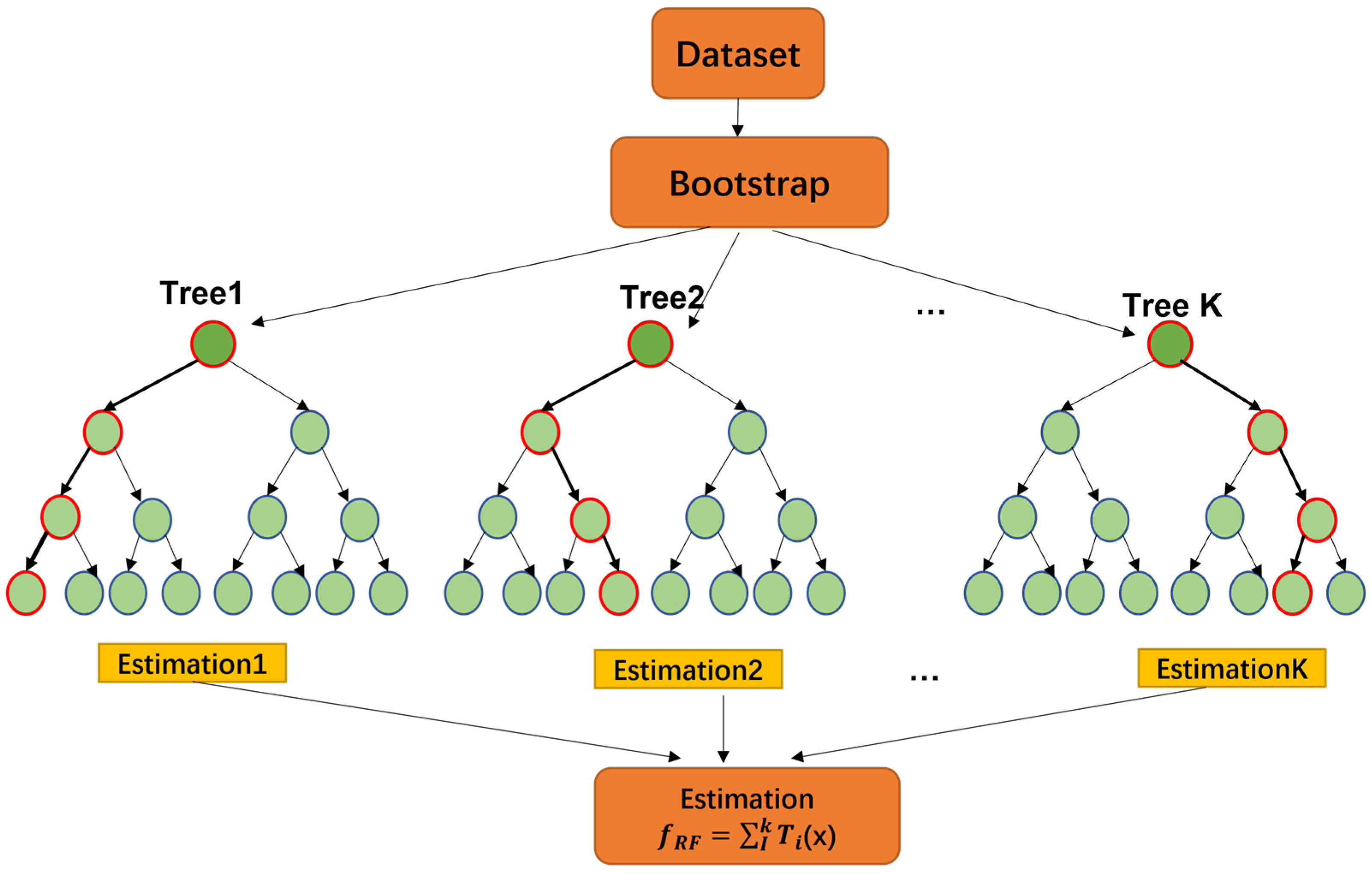
Ensemble learning completes learning tasks by constructing and combining multiple base learners. Boosting and bagging are the most important ensemble learning algorithm models. Bagging randomly samples the original samples and trains the learning model based on the extracted samples. Repeat N times to obtain N base learners, and then obtain the final model by calculating the average error. Boosting is learn multiple weak classifiers by changing the weight distribution of training data and then linearly combining these classifiers to improve overall classification performance.

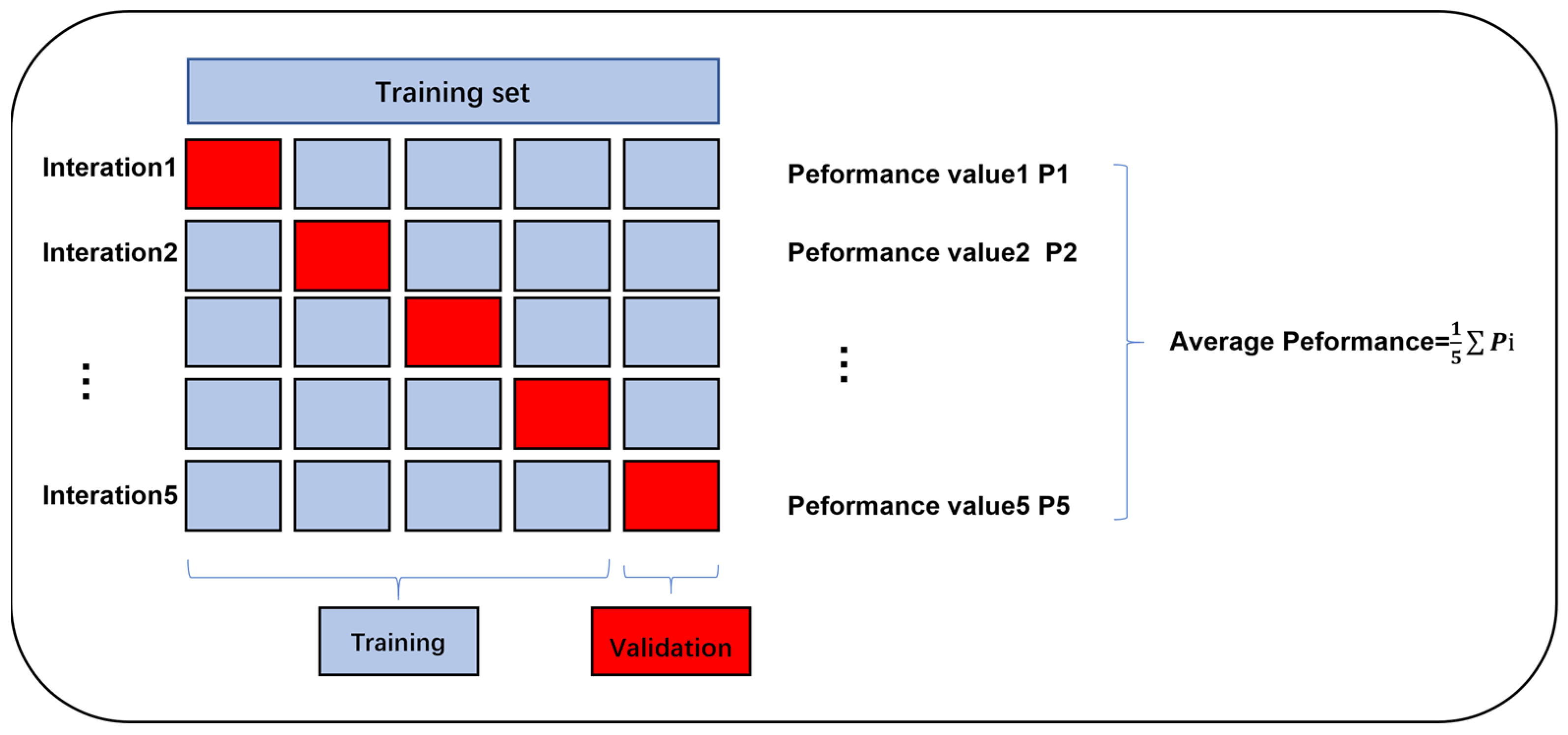
RF and GB are representative models of ensemble learning [30]. Both models are supervised machine learning methods based on decision trees and constructed through integration. In the model training stage, RF, as a typical bagging algorithm, applies random sampling with dropout to the training set for each decision tree. When training a single decision tree, randomly select k features and select the optimal feature from these k features to split the nodes. The training process of RF is shown in Figure 1.

Extra Trees, a variant of RF, was proposed by Geurts in 2006 [31]. Extreme random trees are very similar to random forests, both based on decision trees as the basic unit. Compared to RF, it exhibits a higher level of randomness. When constructing a decision tree, all samples are chosen to train the model, and features are randomly selected during each tree segmentation process. Therefore, the variance of the model will further decrease, but the bias will relatively increase. So the generalization ability of the model may be better than that of random forests in some cases, and to some extent, it can achieve better predictive performance.

The GBDT algorithm is a boosting algorithm that combines GB with CART binary regression trees. This algorithm iteratively learns from the errors made by the previous weak learners to enhance the prediction accuracy. When a prediction error occurs, the learning weight of the sample is increased in the next iteration using the gradient descent algorithm. Consider a training example (X,Y) = {(Xi,Yi)}_i=1^m with m samples, The goal of GBDT is to learn the optimal model F(x) to minimize the specified loss function L(y, f(x)). The procedure of GBDT is as in

Table 1. The procedure of GBDT.

The Procedure of GBDT

Establishes an initial decision tree F0$(x), F_0\left(x\right)=argmin{\displaystyle \sum }_{i=1}^{m}L\left(y_i,c\right)$ When the number of iterations is n times, the residual along the gradient direction can be expressed as: $\widehat{y_i}=-{\left[\frac{\partial L\left(y_i,F\left(x_i\right)\right)}{\partial F\left(x_i\right)}\right]}_{f\left(x\right)=f_{n-1}\left(x\right)}$ $\mathrm{Initialize} \mathrm{the} \mathrm{model} T\left(x_i;\alpha \right)$$\mathrm{by} \mathrm{fitting} \mathrm{sample} \mathrm{data} \mathrm{and} \mathrm{the} \mathrm{parameters} {\alpha }_n$$\mathrm{can} \mathrm{be} \mathrm{obtained} \mathrm{based} \mathrm{on} \mathrm{the} \mathrm{least} \mathrm{squares} \mathrm{method}, {\alpha }_n=argmin{\displaystyle \sum }_{i=1}^m{\left(\widehat{y_i}-\beta T\left(x_i;\alpha \right)\right)}^2$ $\mathrm{Minimize} \mathrm{loss} \mathrm{function} \mathrm{and} \mathrm{update} \mathrm{the} \mathrm{weights} \mathrm{of} \mathrm{the} \mathrm{model}, {\gamma }_n=argmin{\displaystyle \sum }_{i=1}^{m}L(y_i,F_{n-1}\left(x\right)+\gamma T\left(x_i;{\alpha }_n\right)$ $\mathrm{The} \mathrm{final} \mathrm{model} \mathrm{is} \mathrm{updated} \mathrm{as} F_n\left(x\right)=F_{n-1}\left(x\right)+{\gamma }_{n}T\left(x_i;{\alpha }_n\right)$ Meeting the specified number of iterations or termination conditions, the loop will terminate.

2.2. Evaluation Indicators

To compare the accuracy of different algorithms for road rutting prediction, the coefficient of determination (R²), the root mean square error (RMSE), the mean absolute error (MAE), and the mean absolute percentage error (MAPE) were adopted as indicators for evaluating performance. R² represents the proportion of the dependent variable explained by the independent variable; the closer to 1 it is, the better the prediction effect. RMSE represents the deviation between the real and predicted values; the smaller the value is, the closer the predicted value is to the real value. MAE describes the actual error of the predicted value as well as the degree of dispersion of the data. The smaller the value is, the higher the accuracy of the model.

MAPE is a relative measure that utilizes absolute values to avoid positive and negative errors canceling each other out.

$$R^2=1-\frac{{{\displaystyle \sum }}_i^n{\left(y_i-\widehat{y_i}\right)}^2}{{{\displaystyle \sum }}_i^n{\left(y_i-\overline{y}\right)}^2}$$

(5)

$$\mathrm{RMSE}=\sqrt{\frac{{{\displaystyle \sum }}_{i=1}^n{\left(\widehat{y_i}{-y}_i\right)}^2}{n}}$$

(6)

$$\mathrm{MAE}=\frac{1}{n}{\displaystyle \sum }_{i=1}^n|y_i-\widehat{y_i}|$$

(7)

$$\mathrm{MAPE}=\frac{100\%}{n}{\displaystyle \sum }_{i=1}^n\frac{|y_i-\widehat{y_i|}}{y_i}$$

(8)

where n represents the number of samples, y_i represents the test value, and $\widehat{y_i}$ represents the predicted value of the i-th sample. The higher the value of R² is, the lower the RMSE, MAE, and MAPE values, indicating better prediction performance by the model.

2.3. Data Collection

2.3.1. Data from RIOHTrack

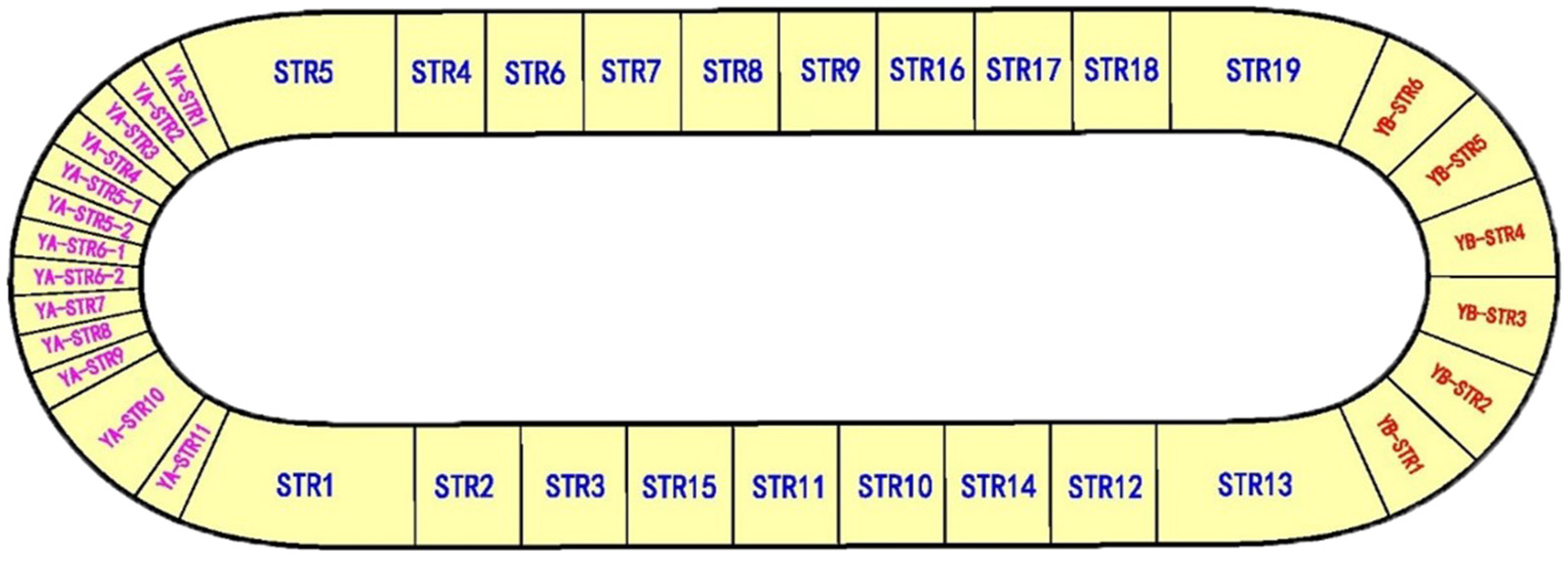
The full-scale pavement track, RIOHTrack, which is based on the climate and geological conditions of North China, was used to study the change law of the service performance (such as rutting) of different pavement structures and materials under the same load. The track has a total length of 2039 m, an elliptical closed curve, and a symmetrical layout. 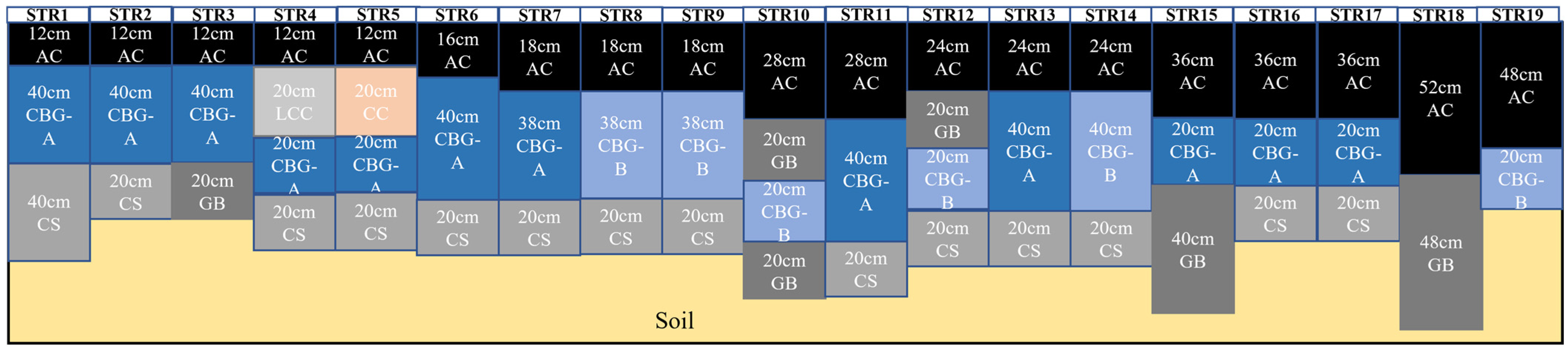It is divided into three parts and 38 test sections (Figure 2). The first part is the main section of the test pavement structure, which covers the straight line and gentle-curve sections of the loop, with a length of 1428 m. A total of 19 types of asphalt pavement structures (STR1–STR19) are laid, from which the rutting data used in this study were primarily obtained. The 19 types of asphalt pavement structures can be divided into four typical structures, namely a rigid base structure, semi-rigid base structure, flexible base structure, and full-depth asphalt pavement (

Table 2. Tested pavement structures.

Type	Struction
Rigid base asphalt pavement	STR1, STR2, STR3, STR6, STR7, STR8, STR9, STR10, STR11, STR12, STR13, STR14
semi-rigid base asphalt pavement	STR4, STR5
Flexible base asphalt pavement	STR15, STR16, STR17
full-depth asphalt pavement	STR18, STR19

). The pavement structure and pavement materials of each test section are shown in Figure 3.

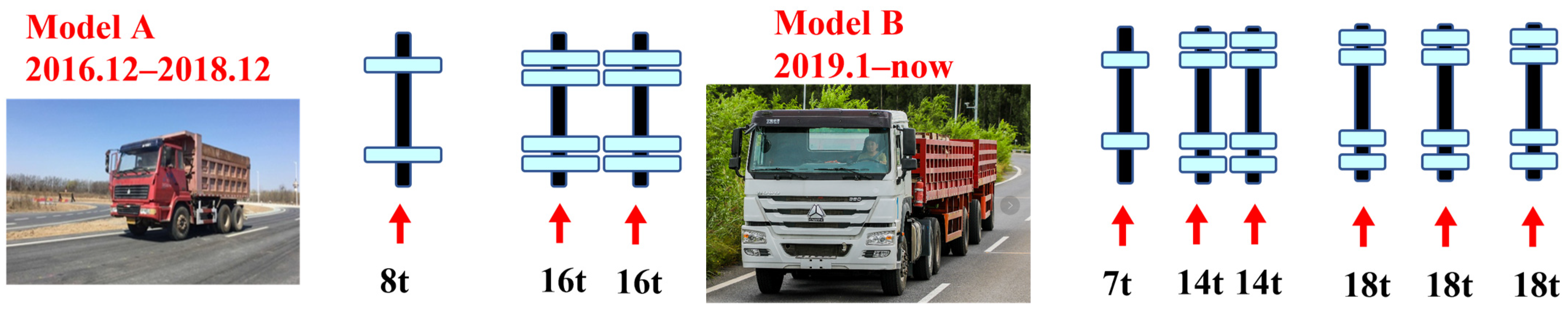
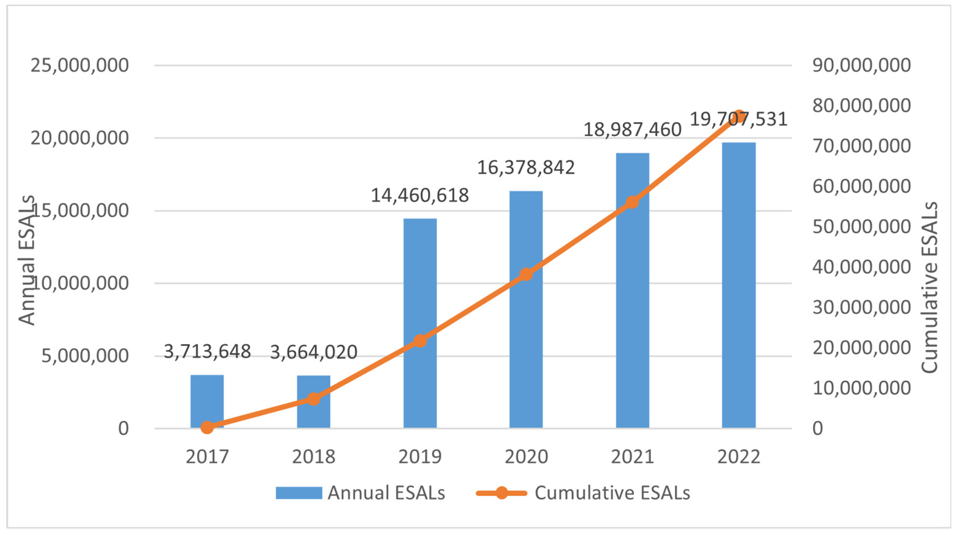
The full-scale track has been loaded and operated since the end of 2016. Four 40-ton Steyr trucks were used for loading. In 2019, they were replaced by six 100-ton trailer trucks. The daily loading mileage was 500 km/vehicle. The vehicle loading mode is shown in Figure 4. The vehicles were operated at a speed of 40–60 km/h, and each loading cycle lasted approximately 11 d. By the end of 2020, the cumulative loading imposed on the track was 2 million kilometers, calculated according to the 4.35 power of the equivalent principle of deflection, which is equivalent to 38 million times the cumulative load on a 10-ton standard axle. The cumulative action times are shown in Figure 5. During the loop loading test, pavement performance metrics, such as rutting, cracking, and skid resistance were measured using a multifunctional inspection vehicle (CICSIII road condition rapid detection system). Simultaneously, climate conditions, including temperature, humidity, and wind, were measured.

2.3.2. Rutting

A multifunctional detection vehicle (CICS) was used to detect the wheel tracks in the lane and obtain data on two-wheel tracks. The method for detecting rutting we used is specified in “Asphalt Pavement Rut Test Regulations”. The detection frequency for each experimental section was set to 5 m, and the average value of all rut depths for this section was calculated as the rut for this section. The maximum rut depth of the left and right wheel tracks were measured and separately calculated, and the average of the left and right rut depths were taken as the rut depth of this experimental section. The rutting data of 19 pavement structures by the end of 2020 were extracted.

2.4. Feature Selection

The input variables, comprising internal and external factors, affect the rutting changes to some extent. The internal factors include pavement structure type and structural layer thickness, as well as modulus, asphalt, aggregate, and mixture properties, whereas the main external factors are the axle load and temperature. The temperature is taken as the daily average temperature during the vehicle loading period. Asphalt type, gradation, and porosity are important to control indicators in the asphalt mixture design process, which greatly affect the anti-rutting performance of the mixture [32]. The input variables after initial selection are listed as follows.

Climate: daily average temperature.

Cumulative axle load: ESALs.

Asphalt mixture upper/middle/lower layers: thickness, modulus, gradation, nominal maximum aggregate size, asphalt penetration, asphalt ductility, asphalt softening point, porosity, asphalt content, and bulk density of asphalt mixture.

Base, subbase, and subgrade: thickness, material type, and modulus.

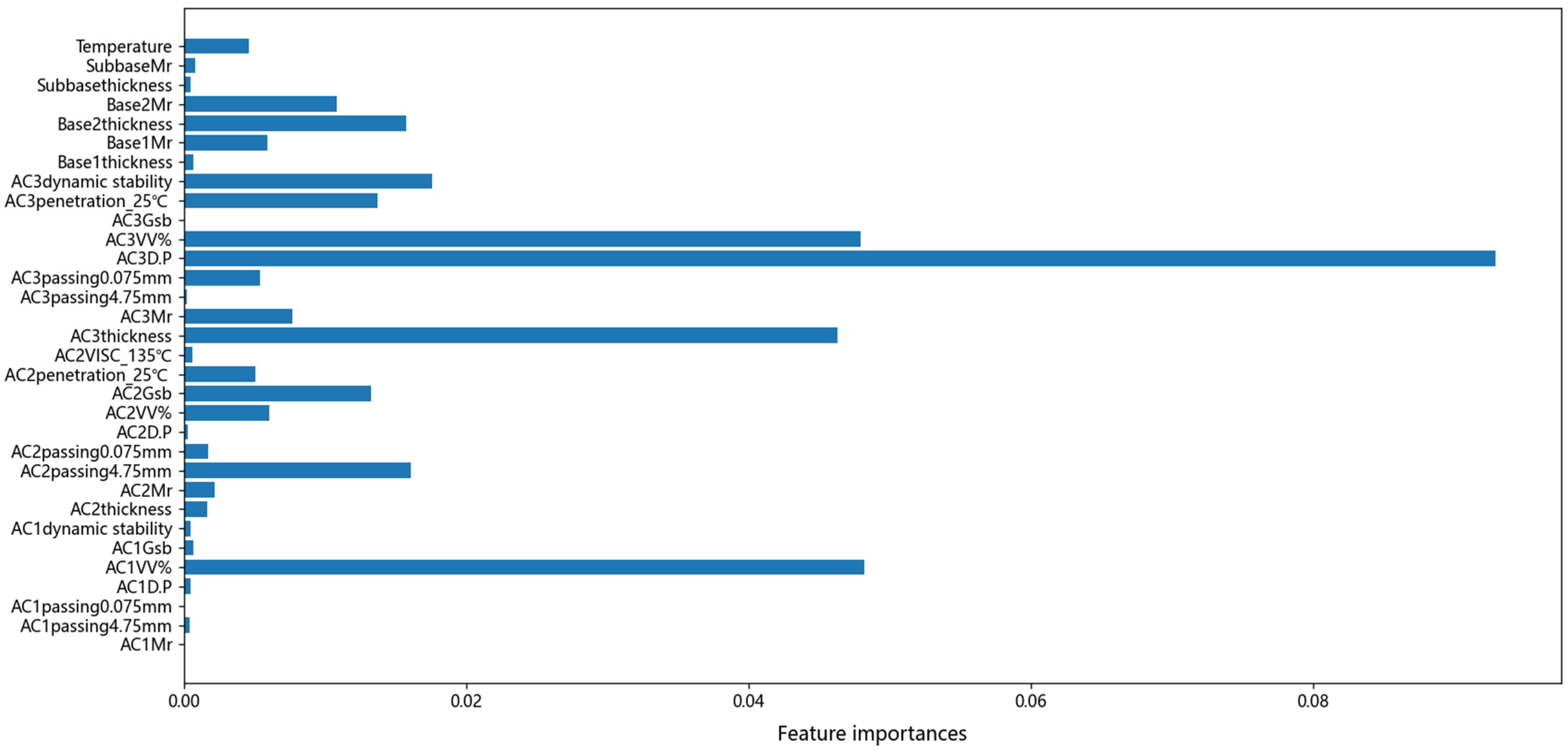
Removing redundant features is crucial as they not only lead to increased computational costs but also affect the computational efficiency of the model and increase the risk of overfitting. Therefore, to improve the computational performance of the model, it is essential to calculate the importance of features and further screen the input variables before training the model. In this chapter, the importance of all variables is calculated using RF, as shown in Figure 6. Thereafter, variables with feature importance of 0 are eliminated, such as AC1penetration_25, AC2dynamic stability, AC3VISC_135, and Subgrade Mr.

Removing unimportant variables does not mean that the remaining variables can be directly used to train the model. It is also necessary to perform multicollinearity diagnosis on the remaining variables and subsequently eliminate any variables exhibiting multicollinearity. This study adopts the reverse elimination method. Reverse elimination is a feature selection method for multiple linear regression, where a significance level of α = 0.05 is first defined, after which all variables are used to fit the model. Next, the variable with the highest p-value is selected and compared with α. If the p-value of the variable is greater than α, the variable is removed. The model is then refitted with the remaining variables, and the process is repeated until all variables are accounted for. The results after variable filtering are listed in

Table 3. Statistical information of variables.

Variables	Min	Max	Mean	Std	Skew	Kurt
AC1Mr	6481	8083	7789	428.7556	−1.6424	2.2024
AC1 passing 4.75 mm (%)	16.4	34.2	30.0	4.6198	−1.3872	1.5642
AC1 passing 0.075 mm (%)	2.2	9.7	7.1052	1.6269	−0.7618	2.4100
AC1D.P	4.29	5.56	5.008	0.3621	0.1112	−0.9678
AC1VV (%)	4.18	13.88	5.33	2.0875	3.5617	11.8116
AC1Gsb	2.3025	2.4919	2.4546	0.0417	−2.4832	6.4980
AC2Mr (MPa)	10,528	17,486	13,940	3310	0.0028	−1.9102
AC2 passing 4.75 mm (%)	24.8	32.1	25.6368	2.0807	0.2630	−0.7595
AC2 passing 0.075 mm (%)	5.4	8.4	6.3421	0.6485	1.4389	2.8774
AC2penetration_25	22.2	63.4	44.8421	19.6062	−0.2422	−1.8696
AC2VISC_135	0.71	2.718	1.9356	0.7661	−0.1036	−1.6625
AC3thickness	0	12	7.2631	5.1600	−0.5472	−1.4564
AC3Mr	0	17218	7990	5861	−0.2806	−1.169
Ac3dynamic stability	0	7701	3071	2615	0.2251	−1.2858
Base2thickness (mm)	12	24	18	3.8942	−0.514	−0.8882
Base2Mr	2000	20,000	4986	5288	2.008	2.331
Subbase thickness (mm)	20	48	23	8.8490	1.9649	2.0135
SubbaseMr	300	20,000	1889	4277	3.9854	13.9700
ESALs(M)	1.04	75.61	28.29	23.90	0.5099	−1.1466
Rutting (0.1 mm)	0	132.1	65.37	23.07	0.3191	−0.3226

.

2.5. Preprocessing

The elimination of outliers within the dataset is crucial for maintaining the integrity and reliability of the data. The popular approaches for outlier detection include probabilistic and statistical modeling, z-score analysis, and box plots. In this study, a kernel density estimation filter was employed to identify such outliers. The proposed method estimates the probability density of each data point and identifies those that have a probability density below a specified threshold(this paper taken 0.05).

The filter was applied to the continuous features, including AC1VV, AC1D.P, AC1Gsb, AC1penetration_25 AC1Dynamic stability, AC2penetration_25, AC2VISC_135, AC3Dynamic stability ESALs (M), and rutting and excluded 38 outliers.

In theory, the number and structure of input variables can affect the model performance. Studying the structure of the variables and optimizing input variables can help improve the precision of the model and lay a foundation for further research. However, categorical variables cannot be directly read by machine learning models, and character data needs to be converted into numerical data. Instead, they can be processed by one-hot vector encoding. In this study, the presence of a stress-absorbing layer is denoted by 1, whereas its absence is denoted by 0. The missing values refer to data that do not exist in the dataset. Due to limitations in detection conditions, collecting complete data is difficult. For instance, due to sensor factors, temperature data on the day of the test (December 2017) were not obtained. Hence, it was replaced by the temperature data of the day before the test. Values whose eigenvalues deviated significantly from the normal range were deleted. The value ranges and measurement units of the feature values in the original data set differed; therefore, they cannot be directly used for analysis. When the difference in each variable is large, if the original value can be directly used for analysis, the role of the variable with a higher value in the comprehensive analysis would be amplified. Similarly, the variables with lower numerical values would have less effect on the output. Thus, to eliminate the degree of impact, all features were standardized before training. Standardization involves scaling the data to a small interval, removing the unit restriction, and converting it into a dimensionless value. In this study, min-max normalization was adopted for the normalization, and mapping to [0, 1] was then conducted as follows.

$$z=\frac{\left(x-x_{min}\right)}{\left(x_{max}-x_{min}\right)}$$

(9)

where z is the standardized value, x is the original data, x_min is the minimum value in the original data, and x_max is the maximum value in the original data.

3. Results and Discussion

3.1. Hyperparameters Selection

Because different hyperparameters may have different effects on the model, the grid search method was adopted to optimize the parameters, and the optimal parameters of the model were screened through cross-validation. The dataset will be divided, with 80% of the data allocated as the training set and the remaining 20% designated as the testing set. It should be emphasized that grid search with cross-validation was performed on the training datasets. Cross-validation [33] randomly divides the training dataset into K parts. K-1 of these subsets are then used for model training, and the remaining datasets are used for evaluation. This process is repeated K times, with each subset acting as the evaluation set once. Finally, the average value of the K test results is determined. For each model, we selected the set of hyperparameters resulting in the highest R² as the optimal value. Consequently, model overfitting can be effectively suppressed and the optimal parameters obtained. This article adopts a 5-fold cross-validation to search for hyperparameters, the process is shown in Figure 7. The mean R² based on a 5-fold cross-validation was used to evaluate the performance of a model.

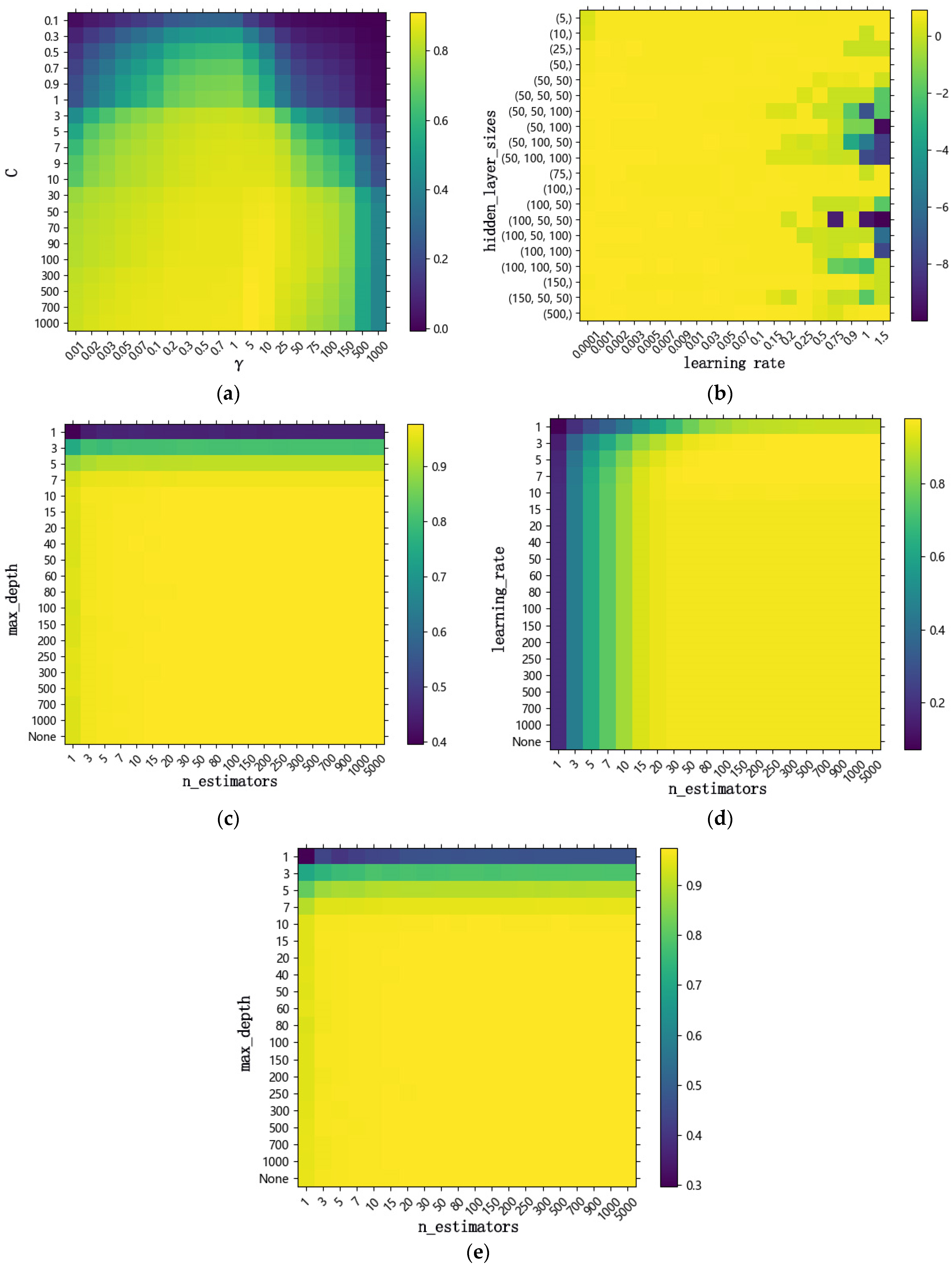
Regarding the selection of hyperparameters in SVR, the kernel function and other parameters can be crucial. ALL the hyperparameters were obtained through 5-fold cross-validation. The form of the kernel function determines the properties of the feature space. Also, different kernel functions correspond to different hyperparameters. The penalty parameter C serves to establish the model’s tolerance for misjudging the target. A higher value of C indicates a lower tolerance for misclassification, resulting in a larger loss function. Epsilon determines the model’s tolerance for errors and controls the smoothness of the regression curve. In general, the larger the epsilon, the higher the smoothness of the model, but the lower the accuracy of the model. The selection of kernel parameters directly governs the model’s fitting ability. With a larger γ, the model becomes more complex and is at a higher risk of overfitting.

Random Forest, GBDT, and Extra Trees are ensemble methods. Ensemble learning is the process of combining several weak learners into one strong learner to improve the performance of a model. The number of estimators (or trees) is a crucial hyperparameter that impacts the accuracy of a model’s predictions. Increasing the maximum number of levels allows the model to gain more information about the data. The number of trees determines the running time of the model. The higher the number of trees, the more times the model needs to be trained. Ensemble learning models are based on decision trees. Max_depth, min_samples_leaf, and min_samples_split are important parameters of a decision tree. The max_depth determines the fitting ability and complexity of the model. An excessive tree depth tends to cause model overfitting.min_samples_leaf represents the minimum number of samples required to construct a decision leaf node. When the number of samples within the node is less than this threshold, pruning operations will be performed. The minimum number of samples required for internal node redistribution (min_samples_split) limits the conditions for the subtree to continue partitioning. The smaller the value, the more refined the model, and the longer the training time. In addition, the learning rate is also important for GBDT, which determines the size of the gradient descent step for each iteration, and a too-high learning rate may cause the model to fail to converge, which determines the rate at which the model reduces the loss function. Too high a learning rate may prevent model convergence.

ANN utilizes many hyperparameters [34], including the number of hidden layers, the number of neurons in each layer, and iterations as well as the activation function and learning rate. The number of hidden layers and hidden neurons are key factors affecting the efficiency of neural networks. The active function affects the output response and model performance.

Table 4. Hyperparameters and mean R² of different methods based on 5-fold cross-validation.

Models	Hyperparameters	Values	Mean R2
SVR	C:	1000	0.9152
	γ	5
	Kernel type	rbf
	epsilon	1
RF	max_depth	None	0.9765
	min_samples_leaf	1
	min_samples_split	2
	n_estimators	300
Extra-trees	max_depth	200	0.9743
	min_samples_leaf	1
	min_samples_split	2
	n_estimators	50
	learning_rate	0.03	0.9800
	n_estimators	250
	max_depth	5
ANN	activation	relu	0.9580
	hidden_layer_sizes	(50, 50, 100)
	learning rate	0.0001
	optimizer	lbfgs

summarizes the evaluation indicators of different algorithm models and the optimal hyperparameters obtained through cross-validation. The search graph for parameters is shown in Figure 8.

3.2. Relationship between Input Variables and Rutting

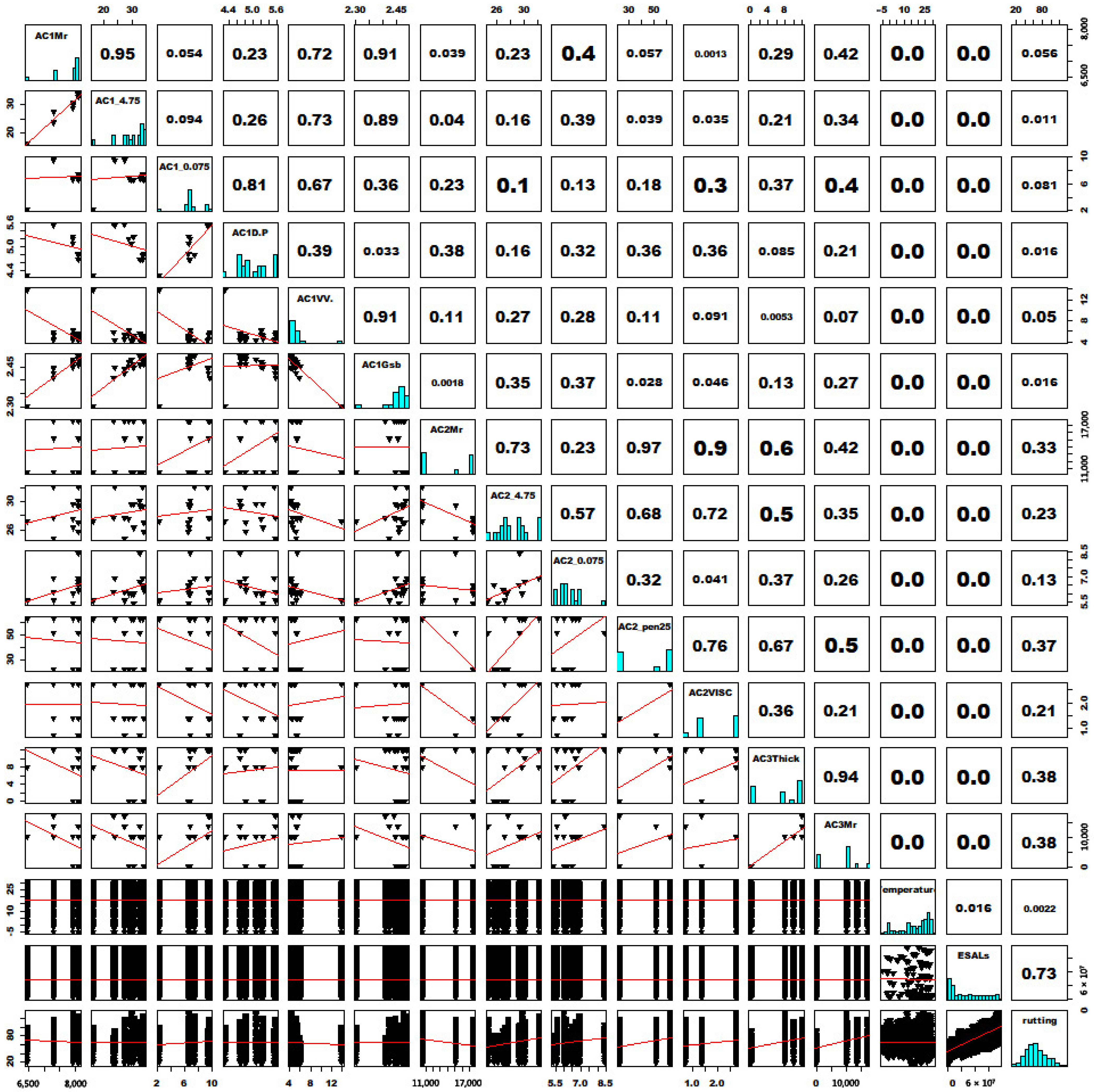
The matrix scatter plot consists of three parts: an upper triangle, a lower triangle, and a diagonal. Each block in the upper triangle represents the correlation coefficients of two variables in the same row and column as the block. The calculation formula is as follows:

$${\rho }_{X,Y}=\frac{cov\left(X,Y\right)}{{\sigma }_X{\sigma }_Y}$$

(10)

where ${\rho }_{X,Y}$ is the Pearson correlation coefficient, $cov\left(X,Y\right)$ is the covariance of two variables, and ${\sigma }_X{\sigma }_Y$ is the standard deviation of the variable. The absolute value of the correlation coefficient indicates the strength of the correlation between two variables. A higher absolute value suggests a stronger correlation between the variables. The lower triangle represents the scatter plot of each pair of variables, and the added line represents a linear correlation trend. Diagonal lines are the histogram that represents the distribution of variables. Figure 9 shows that axle load has the greatest impact on rutting, with a correlation coefficient of 0.73. The impact of temperature is not significant, possibly because the temperature must exceed a certain threshold to have a significant impact on rutting. Therefore, the properties of the lower layer mixture have a greater impact on rutting.

3.3. Performance Comparison

Table 5. Performance indicators of different ML models in test sets.

Model	Performance Indicators
	R2	RMSE	MAE	MAPE
SVR	0.9355	5.9175	3.8224	0.0753
ANN	0.9601	4.6522	3.1729	0.0604
RF	0.9767	3.5570	2.2475	0.0447
GBDT	0.9835	2.9934	1.8687	0.0355
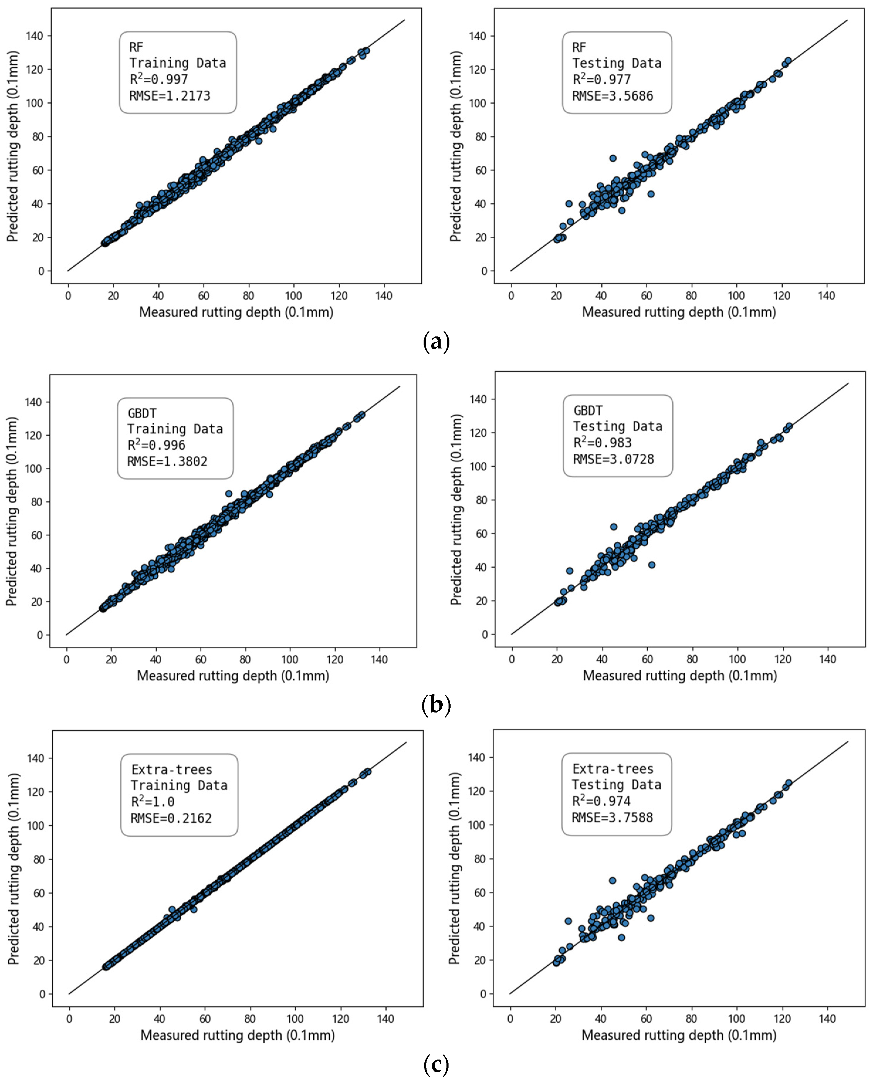
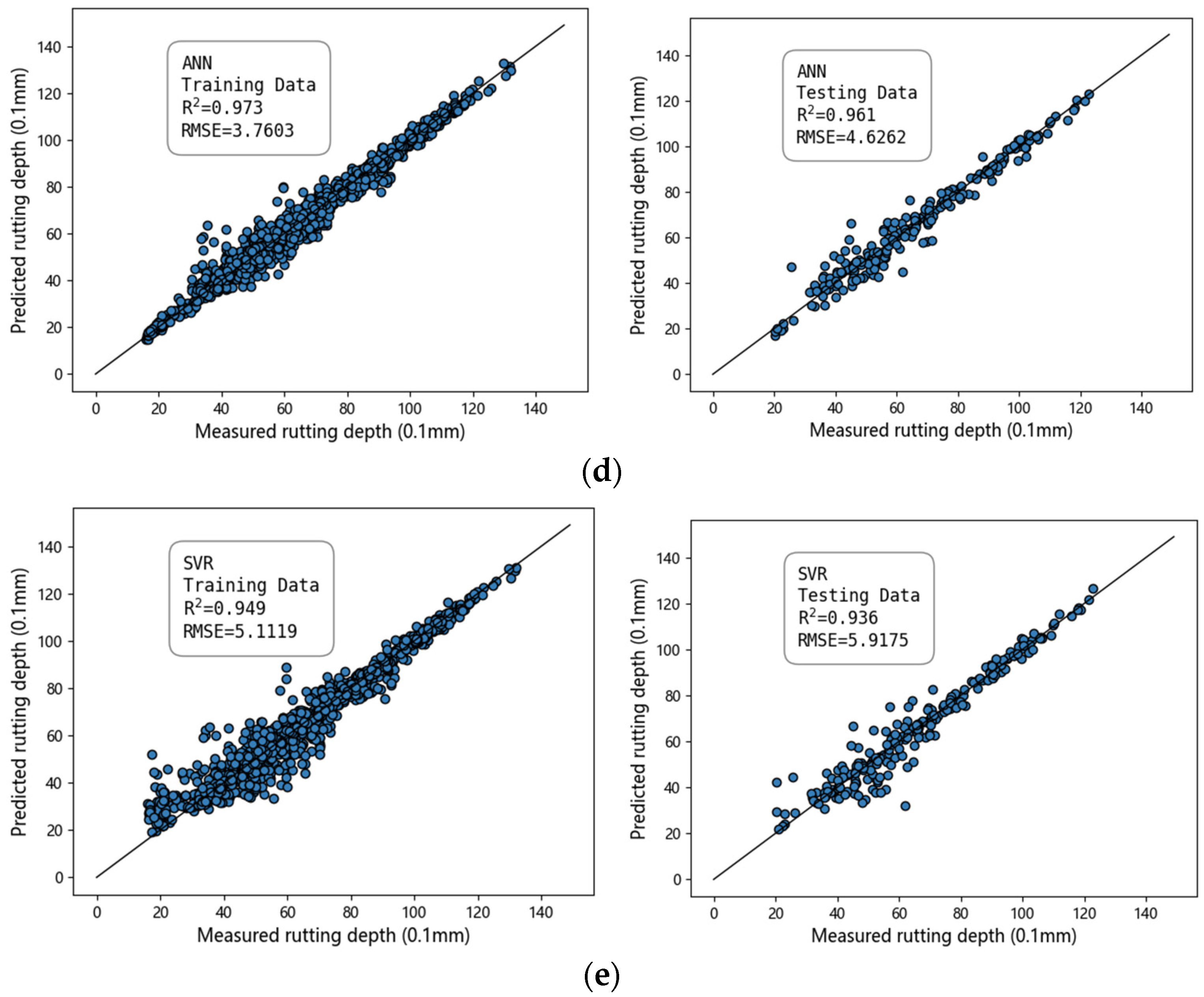
Extra Trees	0.9740	3.7569	2.2937	0.0451

presents the R², RMSE, and MAE values of different prediction models. The higher the value of R² is, the lower the RMSE, MAE, and MAPE values, and the better the model performance. Figure 10 shows the distribution graphs of the predicted and actual values obtained from different algorithms. The more compact the distribution of scattered points around the straight line is, the better the prediction effect. As shown in Figure 8, the tree-based models, namely RF, GBDT, and Extra Trees, demonstrate strong predictive performance, with an R² value of approximately 0.97. However, the training time of the GBDT model was relatively long thrice that of RF and Extra Trees. The prediction performance of ANNs and support vector machines was relatively poor, with R² values of 0.9277 and 0.9346, respectively. This may be attributed to the fact that ANNs require a large amount of data for model training and to improve their accuracy. The limited number of datasets used in this study made it challenging to fully harness the potential performance of neural networks. In contrast, SVR was found to be a weak learner, and prediction performance was also relatively low in this study.

3.4. Comparison with a Mechanistic-Empirical Model

Currently, the M-E rutting prediction models integrated into the pavement are widely utilized by pavement practitioners. Chinese specifications for the design of Highway Asphalt Pavement provide a calculation formula for rutting,

$$R_a={\displaystyle \sum }_{i=1}^n{R}_{ai}$$

(11)

$$R_{ai}=2.31\times {10}^{-8}{k}_{Ri}{T}_{pef}^{2.93}{p}_i^{1.80}{N}_{e3}^{0.48}\left(\raisebox{1ex}{$h_i$}\!\left/ \!\raisebox{-1ex}{$h_0$}\right.\right)R_{0i}$$

(12)

Among them, Ra represents the permanent deformation of the surface layer of the asphalt mixture, R_ai represents the deformation of the i-th layer of the asphalt mixture, n represents the number of layers, and T_pef represents the equivalent temperature of permanent deformation of the asphalt mixture. N_e3^0.48 represents the cumulative number of equivalent axle loads on a lane since the initiation of traffic. It is also referred to as the equivalent single axle loads (ESALs) in this study. Further, h_i is the thickness of the i-th layer (mm), and h₀ is the thickness of the specimen. R is the permanent deformation of the i-th layer of asphalt concrete during the rutting test at a temperature of 60 °C, a pressure of 0.7 MPa, and 2520 loading cycles. K is the correction coefficient, and the calculation formula is as follows:

$$k_{Ri}=\left(d_1+d_2·Z_i\right)·{0.9731}^{Z_i}$$

(13)

$$d_1=-1.35\times {10}^{-4}{h}_a^2+8.18\times {10}^{-2}{h}_a-14.50$$

(14)

$$d_2=8.78\times {10}^{-7}{h}_a^2-1.50\times {10}^{-3}{h}_a+0.90$$

(15)

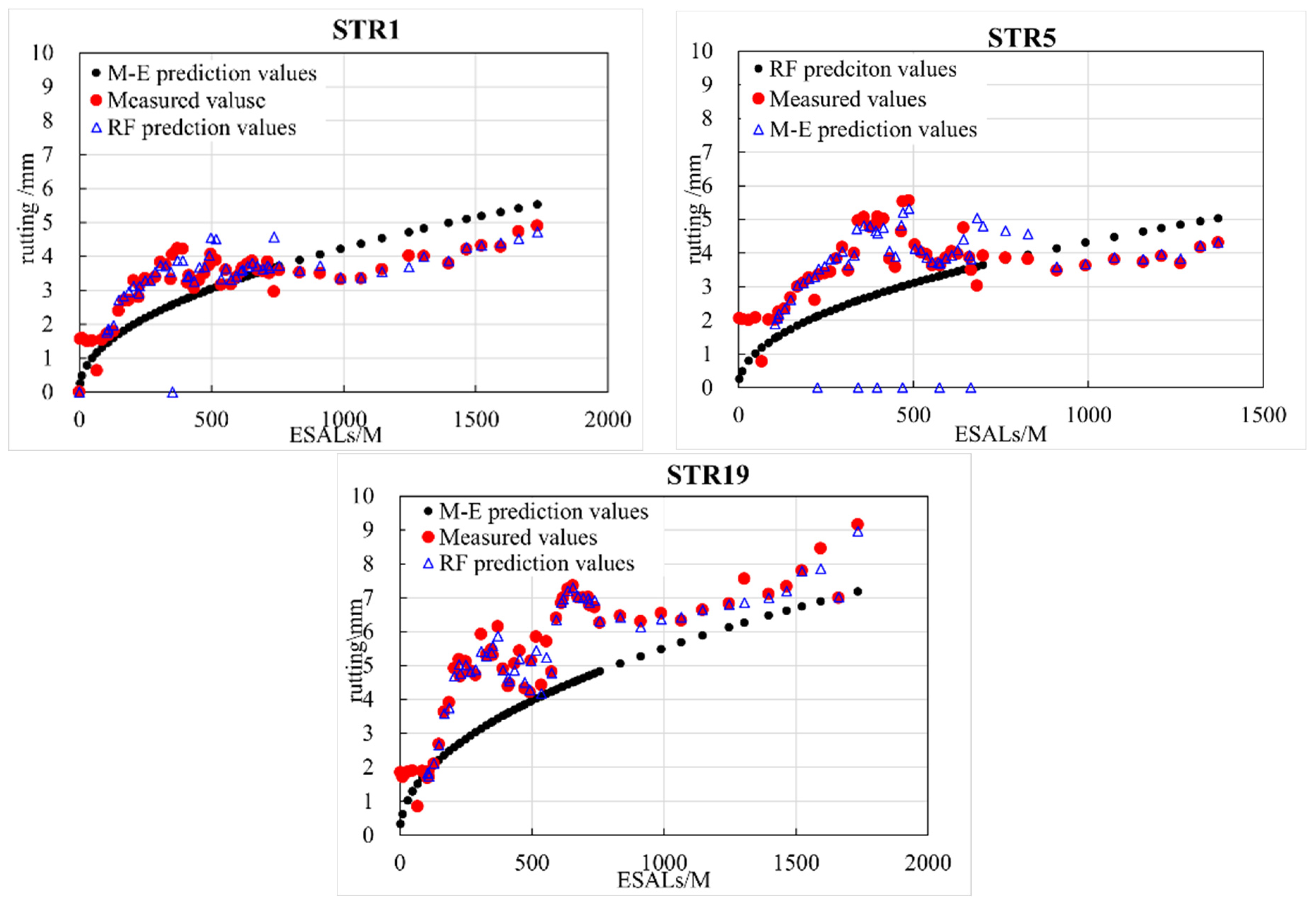
This section utilizes the aforementioned calculation formula to calculate the rut depth of STR1, STR5, and STR9 under different axle loads, which are compared to the rut depths predicted by RF, as shown in Figure 11. The figure shows that the detected rutting depth increases with the increasing ESALs in both prediction models. However, the observed rut depths exhibited an oscillatory increasing trend, but the M-E predicted rutting depth exhibited a monotonic increasing trend, which is not reflective of the actual behavior. The developed GBDT model can achieve higher performance without requiring any local calibration efforts.

The detected rutting tends to peak during the summer months. As winter approaches and ambient temperature decreases, the ruts significantly decrease. This phenomenon can be explained by the density of the asphalt mixture at the rut depressions and bumps being different, which leads to a significant variation in temperature shrinkage performance. In winter, the rutting depressions have a higher density, smaller temperature shrinkage coefficient, and smaller deformation, whereas the bumps have a lower density, larger temperature shrinkage coefficient, and greater deformation. This decreases the difference in deformation between the rut depressions and bumps, resulting in rutting recovery in winter. Tree-based machine learning models, especially RF prediction models, can effectively predict the change patterns of rutting depth, which comprise both linear and fluctuating trends.

The developed GBDT rutting prediction model was compared with other models in terms of generalizability and accuracy. The M-E model is the most widely used in the field of engineering. Before using the M-E model, it is necessary to conduct advanced laboratory testing to obtain the material properties of various asphalt pavement layers. It also needs to carry out locally calibrated work before using. Ref. [35] proposed a variable-order fractional Burgers rutting model by fitting the test data of RIOHTrack. In the paper, rutting can be quantitatively described as the time-varying mechanical deformation, considering the mechanical rheological properties of asphalt mixtures. Ref. [36] proposed a local correction method for the rutting model based on the long-term observation data of RIOHTrack. Both rutting prediction models’ accuracy of all structures is greatly improved but the determination coefficient R² does not exceed 0.95 (R2 in the range of 0.87 to 0.95). While the GBDT model adopted in the paper achieves an R2 of 0.98 without requiring any local calibration efforts. It is difficult to compare the performance metrics of the GBDT model with similar machine-learning models that are available in the literature. Mainly because the dataset on which the model is built is different.

3.5. Analysis of Feature Importance Based on SHapley Additive exPlanations (SHAP)

The analysis of rutting influencing factors can help prevent rutting by controlling key factors. The analysis of feature importance can serve as a simple and effective method for elucidating the interaction between feature and target variables. In order to improve the interpretability of the model, it is necessary to further quantify the impact of feature parameters on rutting performance, and provide more specific guidance for road maintenance management measures. SHAP can provide global and local explanations for the prediction results of GBDT models. Compared with the traditional feature importance based on RF, SHAP can not only rank the importance of each feature affecting the model but also reflect how the features affect the results and their impact trends.

The SHapley Additive exPlanations (SHAP) framework presents an alternative method for evaluating the contributions of various features. It combines game theory principles with local explanations to provide a comprehensive analysis. SHAP can accurately determine the contribution of each feature (${\mathsf{\Phi }}_{\mathrm{i}}$) to the predicted value (f_x) by utilizing the concept of marginal contribution. The formula for calculation is as follows:

$${\mathsf{\Phi }}_{\mathrm{i}}={\displaystyle \sum }_{S\in N\left\{i\right\}}\frac{\left|S\right|!\left(n-\left|S\right|-1\right)!}{n!}\left[f_x\left(S\cup \left\{i\right\}\right)-f_x\left(S\right)\right]$$

(16)

The output target is defined as a linear addition of input features, which can be expressed as:

$$g\left(x\right)={\varphi }_0+{\displaystyle \sum }_{i=1}^m{\varphi }_i{x}_i$$

(17)

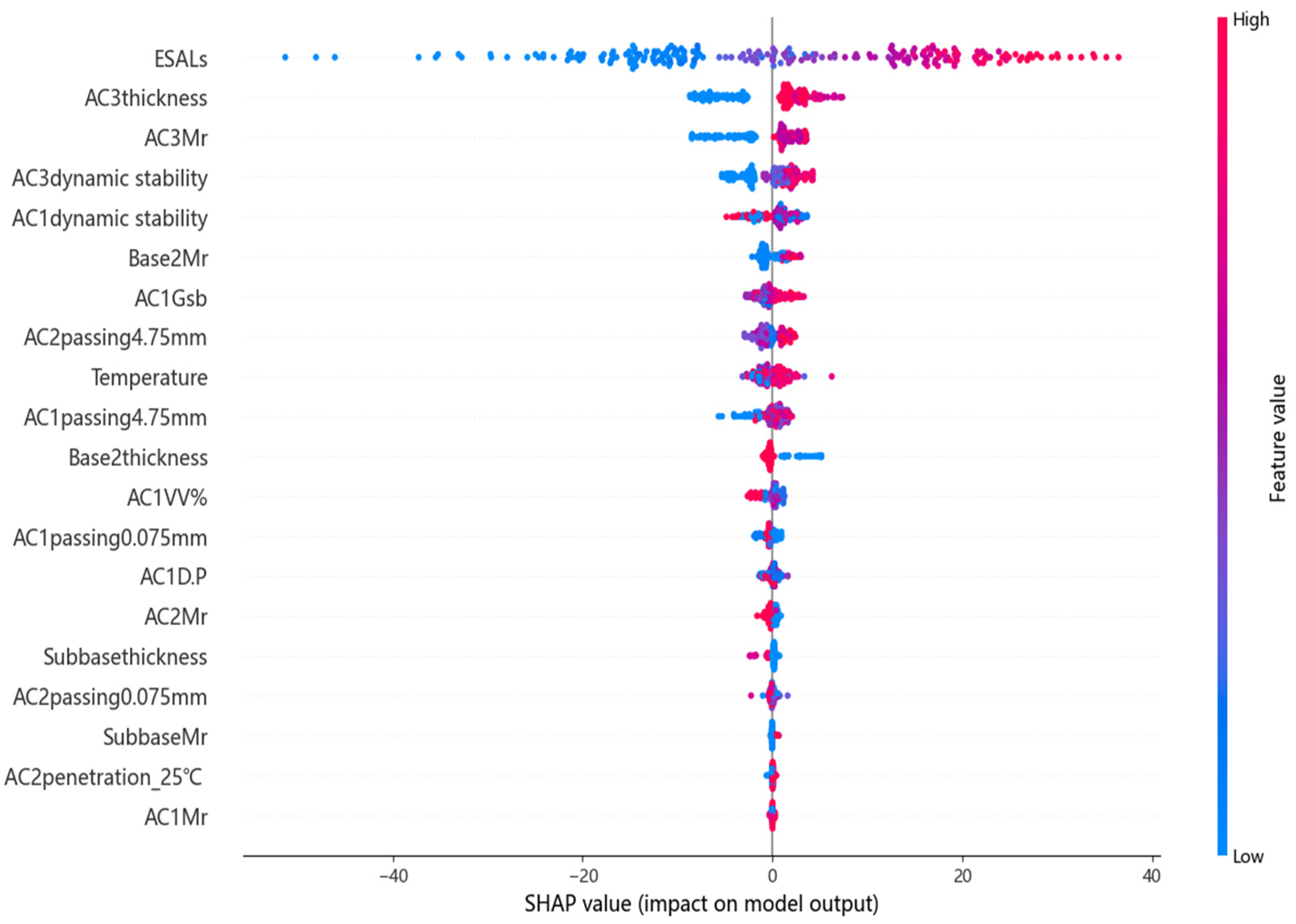
Figure 12 shows scatter density plots of SHAP values of each influence factor. In this graph, each point represents the Shapley value of a feature and a single observation in the dataset [37]. The position of each dot on the x-axis represents the Shapley value assigned to each factor, which indicates its influence on the pavement rutting. Positive values indicate a positive impact, while negative values indicate a negative impact. Additionally, the y-axis provides the factors in their order of importance. The color in Figure 12 represents the values of the factors. For instance, with the high value of base modulus, the asphalt rutting is lower, which indicates us increasing the stiffness of the base is beneficial for reducing rutting depth. However, the influence of ESALS is inverse. The larger the value of ESALS, the value of rutting increases. Feature importance analysis revealed that the material of the asphalt pavement surface layer has a greater contribution to rutting than that of the base and subbase layers. Therefore, rutting research in the future should focus on the performance of surface materials.

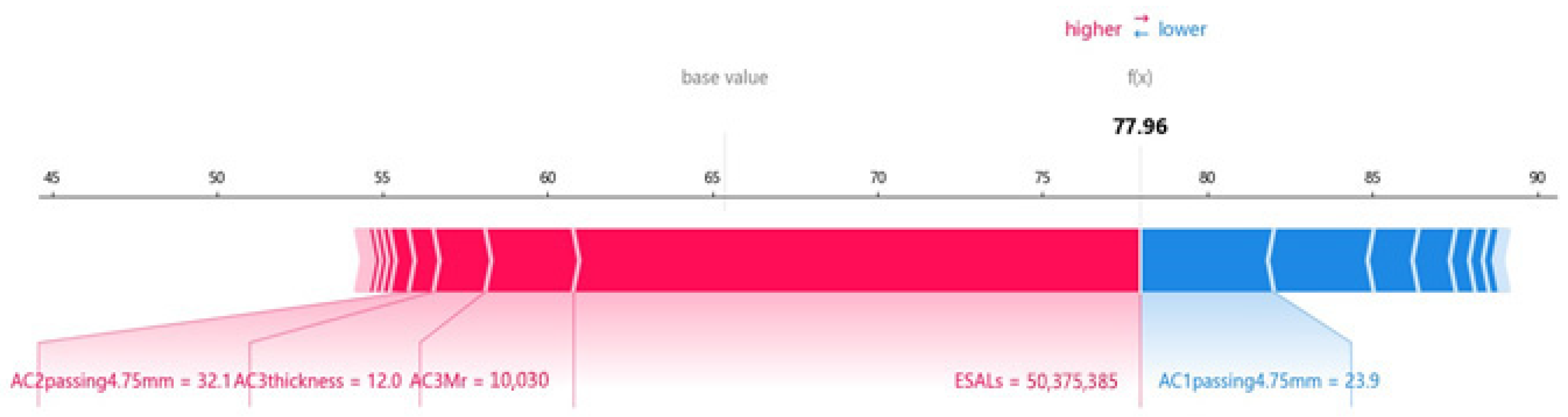
In addition to global interpretation based on the entire dataset, the SHAP method also provides local interpretation for individual samples. Figure 13 shows the Shaply corresponding to each feature and the process from the base value to the final output. In Figure 13, the length of the bar indicates the degree of significance, while the color represents the direction (negative or positive) of each factor’s effect. The mean of the prediction outs is a baseline. It can be seen that ESAL is the most significant factor in infecting rutting.

4. Conclusions

To enhance the accuracy of predicting rutting progression curves for various commonly constructed asphalt pavements in China, this paper utilized five machine-learning methods and data from 19 representative asphalt pavement sections of RIOHTrack. Climate, axle load, the performance of the surface mixture, the thickness of the base and subbase, and modulus, among others, are selected as input variables to train the model. Through careful analysis and discussion of the obtained results, the following conclusions were drawn:

All ML models established in this paper are able to predict rutting well when the hyperparameters are searched thoroughly. Among them, the tree-based ML models such as GBDT, RF, and Extra Trees were proved to have a better prediction ability than SVR (R² = 0.9346) and ANN (R² = 0.9277).

Compared with M-E models, the GBDT model used in the paper provides a high accuracy without any local calibration. More importantly, it can capture the season trend of rutting development. It is also suitable for all structures of RIOHTrack.

After further calculating the SHAP value of the variable, we noticed that the axle load is the core factor affecting rutting. The effect of temperature on rutting is not as obvious as imagined. In addition, for pavement performance, increasing the strength of the base is beneficial for reducing rutting.

The “Design Specification for Asphalt Pavement of Highways” provides corresponding requirements for the allowable rutting deformation of asphalt mixture layers. When the rut depth exceeds the allowable value, timely maintenance measures should be taken. Accurate prediction of rutting depth can take effective control measures for asphalt pavement rutting, thereby improving the highway performance extending the service life of highways, and providing a maintenance reference for asphalt pavement.

This research is mainly based on data mining and statistical methods. Further research should be conducted to apply more mechanism analyses of influence factors on rutting. At present, modeling data are insufficient. In the future, the model will be further adjusted and optimized as the RIOHTRack long-term rutting observation data increases. In addition, the machine learning model proposed in this article should be applied to predict other performances of RIOHTrack, such as cracking and skid resistance. We can also introduce these predicted pavement performance indicators into asphalt mixture mix design.