Abstract
The three-dimensional (3D) reconstruction of Electromagnetic Tomography (EMT) is an important task for many applications, such as the non-destructive testing of inner defects in rail systems. Additionally, image reconstruction algorithms utilizing deep learning methods have been verified to be useful in recent years. Therefore, the interpretability of deep learning is a question that is relevant to its application in other areas. This paper proposes an innovative rotational convolution pattern, Conv-P, for convolutional neural network (CNN) image reconstruction in a 3D EMT system. This pattern is based on the projection relationships inherent in tomographic imaging, where each convolution is performed on adjacent projections along the excitation rotation direction. The advantage of this pattern is that it can generate the convolution process by utilizing the 3D structural information from real sensors. To verify the effectiveness of this convolution pattern, we constructed a 3D dual-layer 16-coil EMT model and tested its image reconstruction performance. The results demonstrate that, compared with two common convolution patterns, Conv-P achieves a 4.7% and 4.1% increase in the Image Correlation Coefficient (CC), a 19.8% and 13.1% reduction in the Relative Image Error (IE), a 0.67% and 1.59% increase in the Peak Signal-to-Noise Ratio (PSNR), and a 3.24% and 0.74% increase in the Structural Similarity Index Measure (SSIM).
1. Introduction
Electromagnetic tomography (EMT), also called magnetic induction tomography (MIT), can reconstruct the distribution of conductivity or permeability to indicate an object’s distribution by detecting the electrical signal around the boundary of the measurement area. Therefore, EMT is a non-destructive detection method with the advantages of being non-contact and non-invasive [1]. Since EMT was proposed, it has been studied in different application fields, including industrial process tomography [2,3], biological tissue imaging [4], and the non-destructive testing of conductive and magnetic materials.
A standard EMT system includes excitation and measurement coils, signal excitation and measurement circuits, and a computing device, such as a personal computer or an embedded system, for image reconstruction. Generally, EMT research includes four directions: the electronic hardware design of the sensor array and signal processing, forward problem calculation, image reconstruction algorithm design, and field application. In recent decades, significant advancements have been achieved in EMT research across these domains. Around the year 2000, different EMT imaging systems were built with a series of explorations, including multiple excitation field designs and signal demodulation methods [5,6,7]. Based on these research efforts, more innovative research has made progress in this field, including faster hardware designs with FPGAs, which significantly increase the image reconstruction speed. Moreover, there have been some new attempts related to magnetic sensor design and image reconstruction algorithms [1,8,9,10]. After 2010, more research began to focus on expanding the application fields and enriching their detection models, such as multi-modality and 3D imaging [11,12,13,14].
1.1. Advancements in 3D Electromagnetic Tomography
Traditional 2D EMT systems non-destructively capture two-dimensional gray-scale images of the measured cross-section. Generally, EMT coils are designed to be installed around the cross-section being measured, which is convenient for generating an excitation field and measuring the shape and size of the target from the tomographic image. Nonetheless, traditional 2D systems face two primary challenges:
- It is impossible to obtain a complete 3D description of the whole object. The present technology is limited to integrating a series of two-dimensional images within the human mind to approximate a three-dimensional structure. Therefore, there is a desire to obtain intuitive and accurate three-dimensional images that display the spatial structure of the object under inspection, providing richer information than two-dimensional images.
- Although the 2D system can reconstruct two-dimensional gray-scale images, the detection targets are definitively distributed in three dimensions. Unlike CT, EMT is a soft field, which means that the image reconstruction process is ill posed. In other words, the reconstructed two-dimensional sectional distribution is influenced not only by the object’s actual distribution on that section but also by the coupling effect of the three-dimensional distribution surrounding the section. In light of this consideration, studying the three-dimensional distribution of the target is a more straightforward process than reconstructing two-dimensional images.
In the preliminary phase of research on 3D EMT, explorations were conducted through both 2.5-dimensional (2.5D) approaches and direct 3D reconstruction. The first approach is pseudo-three-dimensional, or 2.5D imaging, which involves obtaining a series of 2D tomographic images at different radial heights based on 2D image reconstruction methods. Subsequently, the 2D image sequence is processed using contour splicing and Marching Cubes algorithms for interpolation to reconstruct the 3D image. Direct 3D reconstruction can generate images during the reconstruction process by measuring the electrical signal within the same layer and different layers. In contrast to the former, it obviates the need for intermediary steps, such as two-dimensional tomographic imaging and interpolation, that introduce errors.
Our previous work has elucidated the advantages of direct 3D image reconstruction over 2.5D image reconstruction [15]. The EMT sensor has 12 coils, and image reconstruction was performed using the Tikhonov regularization method, the Projected Landweber iterative algorithm, and the total variation regularization method. Wei H.Y. proposed a matrix-free reconstruction method that addresses the problems of large-scale inversion in magnetic induction tomography [13]. Soleimani introduced a numerical solution for solving three-dimensional magnetostatic permeability tomography [16]. In light of the characteristics of metal defects, which are sparse, delicate, and concentrated on the surface, Wang Qi designed a 3 × 3 matrix-distributed sensor array and proposed a sparse regularization method, and they discussed the relationship between the excitation frequency and the detection depth. Simulation and experimental results demonstrate that the total variation regularization algorithm can accurately reconstruct the distribution of sample defects [17]. To improve the central area sensitivity (CAS), Martin Klein designed an excitation coil with spatial undulations, significantly enhancing the CAS by more than 20 dB compared to a traditional circular coil setup [18]. This enhancement allows the central region of a voluminous object with low conductivity to be clearly discernible above the noise floor, a fact that is confirmed by practical measurements. In biomedicine, particularly in the study of cerebral hemorrhage, three-dimensional imaging has been thoroughly investigated. A 3D head MIT simulation model was constructed based on actual CT data, and based on this model, factors affecting the MIT signal were evaluated, as well as factors influencing the safety of MIT devices [19]. Instead of the traditional multi-coil setup, a single coil consisting of several concentric circular wire loops was used for excitation and detection [20]. The feasibility of this method in 3D MIT has also been studied, and it has made breakthrough progress in differentiating tissues in conductivity distribution images of the thoracic spinal column.
1.2. Deep Learning Innovations in Electrical Tomography
Since 2017, research on image reconstruction using deep learning has emerged. Deep learning provides a novel alternative to traditional algorithms that rely on the sensitivity matrix, such as Linear Back Projection, the Tikhonov regularization method, and the Landweber iterative algorithm. Also, deep learning is data-driven, which allows for learning the nonlinear mapping from detection signals to the actual field distribution. It has demonstrated extremely high accuracy in image reconstruction for specific samples or details. In our previous work, two optimized deep learning network structures, a stack sparse autoencoder with a radial basis function network and an optimized fully connected network, were used to achieve the two-dimensional image reconstruction of EMT in simulations. We designed 30,000 samples, including two types: multiple disconnected small objects and a single connected large object. Even after adding 7% noise, the image reconstruction results were relatively excellent [21]. The Restricted Boltzmann Machine, Deep Belief Network, Stacked Autoencoder, and Denoising Autoencoder have all been utilized for the detection of cerebral hemorrhage. The network’s noise resistance performance reached 20 dB [22]. The Restricted Boltzmann Machine has also been applied to the image reconstruction process of EMT, and experimental results have shown that this method has high accuracy. A model-based deep learning network named FISTA-Net was established [23]. After comparing four methods—Laplacian regularization, FISTA-TV, FBPConvNet, and ISTA-Net—FISTA-Net exhibited superior performance and demonstrated good generalization capabilities under different noise conditions.
Following extensive research on deep learning for 2D image reconstruction, some progress was made in the study of deep learning for 3D reconstruction. Convolutional neural networks with a SegNet architecture were utilized for 3D image reconstruction in Electrical Resistance Tomography [24]. The study specifically addressed the influence of various factors on 3D image reconstruction, including the size of the dataset in the training process, data resolution, noise in data feeding, and the characteristics of the training models. Graph Convolutional Networks were applied to 3D Electrical Capacitance Tomography [25]. A unique design of 1012 electric permittivity phantoms was created, with 1000 phantoms for training and 12 for testing. The results showed improvements of 35.5% and 3.74% in the normalized mean square error and Pearson correlation coefficient, respectively. -Net with combined electrodes was used for 3D Electrical Impedance Tomography [26]. Simulations and experiments indicated that -Net exhibited better performance than U-Net. Combined electrodes demonstrated greater robustness than traditional structures and showed superior performance when the signal-to-noise ratio (SNR) was 20 dB or 30 dB.
1.3. Convolution Patterns in EMT: A Projection-Based Approach
In 1998, Yann LeCun et al. developed LeNet-5, the first successful convolutional neural network designed for handwritten digit recognition on the MNIST dataset [27]. In recent years, CNNs have transcended their initial confinement to image processing and have been extensively applied in various domains, such as natural language processing, speech recognition, and medical image analysis. Innovative CNN architectures have been employed in the field of deep learning for Electrical Tomography, in addition to those mentioned in [24,25]. Tan et al. introduced a CNN-based method for image reconstruction in Electrical Resistance Tomography, achieving an impressive Image Correlation Coefficient of 0.95. Moreover, the study enhanced the model’s generalization capability and training speed by exploring adjustments in network architecture, such as the addition of dropout layers and moving averages [28]. Zheng et al. constructed a deep convolutional neural network based on the physical principles of Electrical Capacitance Tomography, which can address both the forward and inverse problems. The network comprises two sub-networks: an encoder consisting of convolutional and pooling layers for estimating capacitance values and a decoder composed of fully connected layers for reconstructing images of the dielectric constant distribution [29]. Chen et al. introduced a CNN-based algorithm for the non-invasive and high-resolution detection of breast tumors through Magnetic Detection Electrical Impedance Tomography. The results indicated that the relative reconstruction error with the CNN algorithm could be reduced to 10% compared to the Truncated Singular Value Decomposition algorithm and the Backpropagation algorithm [30]. Li et al. proposed a Densely Connected Convolutional Neural Network to improve image reconstruction in Electrical Resistance Tomography, effectively mitigating the issues of information and gradient vanishing and significantly enhancing the accuracy and visual quality of the reconstructed images [31]. Wu et al. improved the convolutional neural network approach based on the Visual Geometry Group model by incorporating Batch Normalization layers, ELU activation functions, Global Average Pooling layers, and radial basis function neural networks to accelerate network convergence and improve reconstruction precision and robustness [32]. Kłosowski et al. explored the use of Electrical Impedance Tomography in conjunction with deep learning techniques, specifically convolutional neural networks and Long Short-Term Memory networks, as well as their hybrid models, for detecting moisture distribution within building walls [33].
However, there is scant specialized research concerning the convolution methods applied to the input detection signals, particularly those integrating ET’s unique characteristics. In [28,32], convolution was performed on a 16 × 13 matrix. In [29], convolution was applied to a flattened 1 × 28 vector. Li et al. conducted detailed research on the characteristics of voltage data in Electrical Impedance Tomography. They proposed an image reconstruction method based on one-dimensional convolutional neural networks (1D-CNNs). The experimental results indicated that this network significantly outperforms traditional DNNs and 2D-CNNs in terms of image reconstruction quality [34]. The authors also elucidated the reasons why 1D-CNNs are superior to 2D-CNNs. An excerpt from their discussion states, ’It is time-consuming for converting 1D samples to 2D. Furthermore, the structure of the original measurement signal may be destroyed so that incorrect features may be extracted from 2D signals.’ Building upon this work, we wish to further explore the physical significance behind the fact that the correlation of signals is destroyed after converting 1D samples to 2D. To this end, it is necessary to trace back to the origins and fundamental concepts of the two technologies, CNN and tomography.
In 1959, experiments conducted by Hubel and Wiesel on the visual cortices of cats revealed that specific cortical neurons were susceptible to edges or stripes of specific orientations, laying the biological foundation for the subsequent development of convolutional neural networks [35]. Inspired by the cognitive processes of animal vision, the CNN eliminates the one-to-one connections between specific pixels, adopting a convolutional kernel to implement a weight-sharing mechanism. This change uses the high correlation between adjacent pixels in images, reducing the number of network parameters while preserving the characteristics of pixel connectivity. For the convolution of EMT detection signals, it is necessary to examine the characteristics of EMT in order to select the appropriate convolution method for them.
In 1917, the Radon transform laid the theoretical foundation for tomographic imaging [36]. Tomographic imaging is a technique that reconstructs internal structures by collecting projection data that pass through an object from different angles. The concept of projection is significant in the tomographic imaging process. Physically, it refers to the measure of changes in the detected signal values due to the presence of the object when an excitation signal passes through the object in a particular direction (linear or nonlinear). Each projection contains information as seen from a specific angle but is insufficient to reconstruct the structure of the object being measured independently. These projection data are collected and used to reconstruct the internal image of the object through mathematical algorithms. The core of tomographic imaging lies in integrating these projection data from different angles to reconstruct a complete internal structure.
Figure 1 describes the sensitivity regions of projection , projection , and projection in an eight-coil EMT system. Taking projection as an example, the notation refers to the configuration where coil 1 serves as the excitation source and coil 3 serves as the detector. From Figure 1, it can be seen that projection has an overlapping sensitivity region with projection . However, projections and hardly have overlapping sensitivity regions.
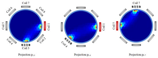
Figure 1.
Three projections: , , and .
From this, we can infer that it may be inappropriate to convolve projection with projection together, as they are not adjacent in physical space, so such an approach would fail to provide commonalities and be prone to extracting erroneous features. Thus, the 1D-CNNs and 2D-CNNs in [34] were reanalyzed. Because the input signals of 1D-CNNs and 2D-CNNs are distributed through signal acquisition, there is no second design. Between the two, 1D-CNNs use more adjacent projections to participate in convolution than 2D-CNNs (the use of projection by 2D-CNNs is also chaotic), which is consistent with the better image reconstruction effect of 1D-CNNs compared to that of 2D-CNNs. However, careful observation shows that 1D-CNNs do not make good use of all adjacent projections to participate in convolution, and non-adjacent projections participate in convolution. This may be the physical interpretation of the process.
In summary, there is limited research on deep learning for 3D ET, especially EMT. Compared to the classic 2D image reconstruction algorithms for 3D image reconstruction, deep learning offers an end-to-end approach, a more direct method for 3D image reconstruction. Convolutional neural networks extract standard features by exploiting the spatial correlations of adjacent elements. If this process could be integrated with the intrinsic relationships between the projections of EMT itself, it would likely result in a convolution pattern that is more suitable for EMT applications. However, research on this topic is scarce, and it merits further investigation. For this reason, this paper proposes a rotational convolution pattern, ’Conv-P’, which utilizes adjacent projections for convolution, applicable to 3D EMT.
2. Theory and Model
This section mainly introduces the fundamental theories of EMT, as well as the EMT model and convolutional neural networks used in this paper.
2.1. EMT Theory
In EMT, the displacement current can be ignored when the excitation frequency is low . Inserting into Maxwell’s equations results in
Considering electromagnetic induction, ignoring the electric field component caused by a potential change , it can be considered that
Equation (3) describes how the vector magnetic potential changes in EMT under a given conductivity and permeability distribution.
If the permeability does not depend on the internal change, we consider to be a constant . According to the vector identity , in the case of Coulomb gauge , the above formula can be written as
This simplified Equation (4) describes how the vector magnetic potential changes in EMT under a given conductivity distribution in EMT.
2.2. The 16-Coil 3D EMT Model
Because multi-layer sensors can provide more projections between different layers, such sensors are more suitable for 3D imaging. Taking scalability into account, we referenced the classic 8-coil EMT model and constructed a dual-layer, 16-coil model with 8 coils per layer, as illustrated in Figure 2. In Figure 2, the green parts represent the coils, while the gray sections indicate the tube.
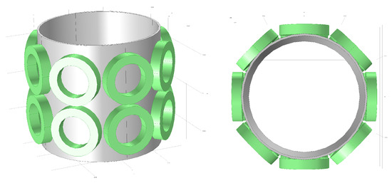
Figure 2.
Dual-layer 16-coil configuration for 3D Electromagnetic Tomography System.
By sequentially exciting and detecting through 16 coils, a two-dimensional matrix can be created with 256 projections. Suppose considerations for the removal of information redundancy are taken into account. In that case, the Reciprocity Theorem stipulates that the outcome of coil i acting as the exciter and coil j as the detector is equivalent to that when coil j is the exciter and coil i is the detector.
Upon excluding all self-induction signals , a total of independent detection signals are obtained.
2.3. Convolutional Neural Networks
With the advancement of deep learning, the needs of traditional industrial and biomedical applications have expanded into a broader algorithmic realm. This article’s CNN network architecture is shown in Figure 3. It has been demonstrated that a single convolutional layer can achieve satisfactory image reconstruction results, thereby negating the necessity for additional convolutional layers.
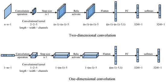
Figure 3.
Traditional CNN structures of one-dimensional and two-dimensional convolutions.
Both one-dimensional and two-dimensional convolutions are utilized for the image reconstruction process. The input for the one-dimensional convolution is a input vector processed through a convolutional kernel of size (length × width × number of channels). The input for the two-dimensional convolution is an matrix processed through a convolutional kernel of size (length × width × number of channels). Subsequently, a convolution operation with a stride of 1 is performed, followed by activation through the ReLU activation function. Given the low dimensionality of the input, no down-sampling is performed. The data are then passed through a fully connected network, and the output is a 3240-dimensional distribution of 3D space after a softmax function:
In this study, the loss function employed is the cross-entropy loss function. Through the utilization of softmax mapping, it establishes associative relationships between various outputs while concurrently expanding the distance between them. This approach aims to maximize the probability values of outputs that contain the object, thereby facilitating the imaging operation. denotes the cross-entropy, which is expressed as follows:
Here, denotes the actual distribution within the element, while represents the predicted distribution for the same element. n signifies the total number of elements, which amounts to 3240 in this study.
3. The Design of the New Rotational Convolution Pattern
As analyzed previously, the design of convolution patterns is crucial for CNN applications. In this part, we compare three convolution patterns and study their impacts on the quality of image reconstruction. Regarding samples, three different sizes of solid spheres with radii of 6 mm, 7.5 mm, and 15 mm are selected as imaging objects. The samples can contain one sphere or two spheres. A total of 31,476 samples were generated and distributed in a ratio of . The data in each set are non-repetitive. The data in the validation set are only used to adjust the network’s hyper-parameters during training and do not participate in testing. The data of the test set will only be used in the final testing phase.
3.1. Comparison of Convolution Patterns
When applying a CNN to EMT, the targets of convolution are the detection signals collected by the sensors, namely, the different projections. These signals are arranged according to the order of acquisition, without a special secondary design for convolution. For clarity, we chose to set the total number of coils to 5 in Figure 4, Figure 5 and Figure 6, aiming to make the convolution pattern descriptions more intuitive. Nonetheless, the entire process is consistent with the 16-coil EMT model in this article.
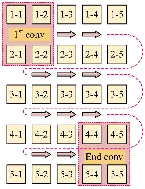
Figure 4.
Convolution pattern: Conv-A.
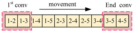
Figure 5.
Convolution pattern: Conv-B.
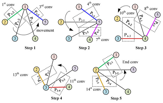
Figure 6.
Rotational convolution pattern: Conv-P.
Typically, the process involves two conventional patterns: a two-dimensional convolution pattern and a one-dimensional convolution pattern. Figure 4 illustrates the conventional two-dimensional convolution pattern termed ‘Conv-A’, which involves sequential convolution over a matrix region, moving from left to right and top to bottom, executing a total of convolution operations, where n represents the number of coils.
Figure 5 shows the normal one-dimensional convolution pattern, termed ‘Conv-B’ in this paper, which consists of executing convolution sequentially over a region of a vector. In practice, the normal one-dimensional convolution operation is performed on a one-dimensional vector, with a total of convolution operations conducted.
It is observed that part of the convolution process in Conv-A and Conv-B is chaotic. In Conv-A, many adjacent projection combinations do not participate in convolution. In Conv-B, after the convolution of and is completed, must be followed by , and the two projections and are not adjacent. Therefore, we refer to the development of CNN, how it works in image recognition, and the reconstruction mode of tomography (this part has been described in Section 1.3). Building on these insights, we introduce a rotational convolution pattern with projection design termed ‘Conv-P’.
In Figure 6, the convolution process, according to the logical working principle of EMT, is depicted in five steps. Starting with Step 1, convolution begins with the projection from to , using coil 1 for excitation. Since the previous step concluded with the projection direction , Step 2 begins at this point, ensuring continuity by concatenating the convolution related to coil 1 with that of coil 5. Consequently, the excitation shifts from coil 1 to coil 5. The convolution proceeds from to and concludes at , indicating that the sequential convolution involving coil 5 is completed. This process is repeated through three additional steps, with each convolution movement between steps being rotational in the spatial projection. Notably, in Step 5, the final projection is , which coincides with the initial projection from Step 1, thus creating a closed loop. Therefore, from Step 1 to Step 5, a total of convolution operations are executed.
3.2. Reconstructed Images
The simulation environment is the multiphysics software from COMSOL 5.4. The network is constructed and implemented in PyCharm based on the TensorFlow environment. Upon establishing the network, we implement the image reconstruction process in two steps. First, we train the network with a pre-determined training set and then use the test set to test the results on the trained network.
The evaluation parameters for reconstructed images are the Image Correlation Coefficient (CC), the Relative Image Error (IE), the Peak Signal-to-Noise Ratio (PSNR), and the Structural Similarity Index Measure (SSIM).
Here, g denotes the vector of the actual distribution (the ground truth), while represents the vector of the predicted distribution (reconstructed image). Both g and have dimensions of . is the maximum possible pixel value of the image (in this paper, it is 1). is the average value of the actual distribution. is the average value of the predicted distribution. is the variance of the actual distribution. is the variance of the predicted distribution. is the covariance between the actual distribution and the predicted distribution. are small constants added to avoid division by zero.
Reconstructed images with higher imaging quality generally tend to have higher CCs, lower IEs, higher PSNRs, and higher SSIMs. Table 1 presents the average values of the CC, IE, PSNR, and SSIM across all training and testing sets.

Table 1.
The evaluation parameters of reconstructed images.
In terms of imaging quality metrics, the efficacy of the convolution patterns is ranked as follows: Conv-P > Conv-B > Conv-A. The superiority of Conv-P over Conv-B suggests that the rotational convolution pattern with projection design is more adept at utilizing the spatial projection information inherent in the EMT sensing modality. This approach can provide the CNN with more spatial structural information from the sensors.
The fact that Conv-B outperforms Conv-A indicates that the current one-dimensional convolution pattern is more effective in imaging than the two-dimensional approach, possibly because the latter does not adequately exploit the spatial projection information of EMT. In Conv-A, signals with low correlations may be convoluted together, contributing to effective feature extraction.
However, it is noteworthy that the differences among Conv-P, Conv-B, and Conv-A are not substantial. If a 3D industrial application requires faster computing speed, and if Conv-B’s imaging accuracy meets on-site demands, then Conv-B could also be a viable option. This is especially relevant considering that Conv-P has nearly twice the number of parameters compared to Conv-B. Additionally, within this sample set, it can be observed that the training set achieves slightly higher quality compared to the test set. The slight difference hints at the model’s ability to adeptly learn the distribution mapping from sensor signals to sample representations.
For a statistical analysis of the process, we employed the Mann–Whitney U test. Given the large sample size (3147 samples in the test set), the normal approximation was used for p-value computation. The mean () and standard deviation () of the U distribution were calculated using the following equations:
Here, and represent the sizes of the two comparative sample groups. The Z-score was determined by taking the observed U value, subtracting , and then dividing by :
This Z-score was subsequently utilized to ascertain the corresponding p-value from the standard normal distribution. A p-value less than 0.05 indicates a statistically significant difference between the two sample groups. The obtained p-values are shown in Table 2 after the calculations.
Table 2.
The p-values between Conv-A, Conv-B, and Conv-P.
These results indicate statistically significant differences among Conv-A, Conv-B, and Conv-P. The exceedingly small p-values strongly affirm the presence of distinct statistical disparities between Conv-A, Conv-B, and Conv-P.
The specific reconstructed images are presented in Figure 7. It can be seen that the CNN for three-dimensional image reconstruction in EMT is feasible. The detection signals from the 16 coils in three dimensions indeed contain information about the three-dimensional distribution of the objects. The CNN network in this paper could learn this relationship and reconstruct images of reasonable quality. As observed in Figure 7, the objects in the reconstructed images are generally clustered rather than dispersed, indicating good performance. This outcome is also related to the choice of loss function employed. Moreover, it can reconstruct positional, size, and shape information for various object configurations, including a single small sphere, a single large sphere, and a combination thereof.
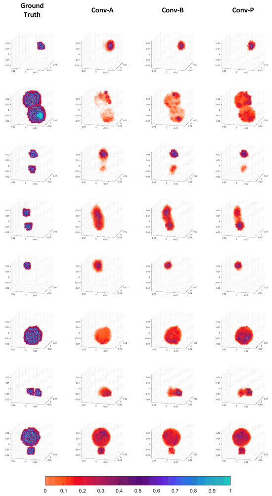
Figure 7.
Three-dimensional reconstructed images.
The reconstructed images also demonstrate that, compared to the Conv-A and Conv-B patterns, the Conv-P pattern performs better-quality image reconstruction. For instance, in the reconstructed image of the second sample, the completion and filling in of the volume of two large spheres can be observed as the process progresses from Conv-A to Conv-B and then to Conv-P. In the fifth sample, there are also some peripheral artifacts in Conv-A. The reconstructed images of Conv-B and Conv-P are almost consistent with the ground truth. In the reconstructed images of the fourth and seventh samples, the two objects that are nearby appear to be fused in the Conv-A and Conv-B patterns. In contrast, the distinction between the two objects is noticeably more apparent in the Conv-P reconstruction. Therefore, the image quality of the Conv-P reconstruction has improved compared to that of the Conv-A and Conv-B patterns. This suggests that the rotational convolution pattern with projection design positively enhances the image reconstruction quality.
4. Conclusions
This paper introduces an innovative convolution pattern design tailored for 3D EMT image reconstruction using a CNN. This convolution pattern, Conv-P, constructs a convolutional route using the real sensor 3D structure information and the logical EMT rotational projection sequence. A dual-layer, 16-coil 3D EMT model was built to test the proposed rotational convolution. Compared with the 2D EMT model, the dual-layer 3D model has a more significant sensor spatial structure. Simulated reconstructions of the distributions with different object configurations were performed with Conv-P. The results show that Conv-P on this testing model can increase the quality of image reconstruction with evaluation indicators. This result demonstrates that designing a convolution pattern according to a real system’s structure and logical working principle is a reasonable method.
Author Contributions
Conceptualization, P.Z.; methodology, P.Z. and Z.L.; software, P.Z.; validation, P.Z.; formal analysis, P.Z. and Z.L.; investigation, P.Z.; resources, P.Z. and Z.L.; data curation, P.Z.; visualization, P.Z. and Z.L.; supervision, P.Z. and Z.L.; project administration, Z.L.; funding acquisition, Z.L.; writing—original draft, P.Z. and Z.L.; writing—review and editing, P.Z. and Z.L. All authors have read and agreed to the published version of the manuscript.
Funding
The work is supported by the National Key Research and Development Program of China under Grant 2020YFC2200704.
Institutional Review Board Statement
Not applicable.
Informed Consent Statement
Not applicable.
Data Availability Statement
The data presented in this study are available upon reasonable request from the authors.
Conflicts of Interest
The authors declare no conflicts of interest.
References
- Yin, W.; Peyton, A.J. A planar emt system for the detection of faults on thin metallic plates. Meas. Sci. Technol. 2006, 17, 2130. [Google Scholar] [CrossRef]
- Ma, L.; Soleimani, M. Hidden defect identification in carbon fibre reinforced polymer plates using magnetic induction tomography. Meas. Sci. Technol. 2014, 25, 055404. [Google Scholar] [CrossRef]
- Terzija, N.; Yin, W.; Gerbeth, G.; Stefani, F.; Timmel, K.; Wondrak, T.; Peyton, A.J. Use of electromagnetic induction tomography for monitoring liquid metal/gas flow regimes on a model of an industrial steel caster. Meas. Sci. Technol. 2010, 22, 015501. [Google Scholar] [CrossRef]
- Zakaria, Z.; Rahim, R.A.; Mansor, M.S.B.; Yaacob, S.; Ayub, N.M.N.; Muji, S.Z.M.; Rahiman, M.H.F.; Aman, S.M.K.S. Advancements in transmitters and sensors for biological tissue imaging in magnetic induction tomography. Sensors 2012, 12, 7126–7156. [Google Scholar] [CrossRef] [PubMed]
- Peyton, A.J.; Yu, Z.Z.; Lyon, G.; Al-Zeibak, S.; Ferreira, J.; Velez, J.; Linhares, F.; Borges, A.R.; Xiong, H.L.; Saunders, N.H.; et al. An overview of electromagnetic inductance tomography: Description of three different systems. Meas. Sci. Technol. 1996, 7, 261. [Google Scholar] [CrossRef]
- Korjenevsky, A.; Cherepenin, V.; Sapetsky, S. Magnetic induction tomography: Experimental realization. Physiol. Meas. 2000, 21, 89. [Google Scholar] [CrossRef] [PubMed]
- He, M.; Liu, Z.; Xu, L.J.; Xu, L.A. Multi-excitation-mode electromagnetic tomography (emt) system. In Proceedings of the 2nd World Congress on Industrial Process Tomography, Hannover, Germany, 29–31 August 2001; pp. 247–255. [Google Scholar]
- Yin, W.; Chen, G.; Jiang, J.; Cui, Z. The design of a fpga-based digital magnetic induction tomography (mit) system for metallic object imaging. In Proceedings of the 2010 IEEE Instrumentation & Measurement Technology Conference Proceedings, Austin, TX, USA, 3–6 May 2010; pp. 363–366. [Google Scholar]
- Soleimani, M.; Lionheart, W.R.B. Absolute conductivity reconstruction in magnetic induction tomography using a nonlinear method. IEEE Trans. Med Imaging 2006, 25, 1521–1530. [Google Scholar] [CrossRef] [PubMed]
- Palka, R.; Gratkowski, S.; Stawicki, K.; Baniukiewicz, P. The forward and inverse problems in magnetic induction tomography of low conductivity structures. Eng. Comput. 2009, 26, 843–856. [Google Scholar] [CrossRef]
- Zhang, M.; Ma, L.; Soleimani, M. Dual modality ect–mit multi-phase flow imaging. Flow Meas. Instrum. 2015, 46, 240–254. [Google Scholar] [CrossRef]
- Ma, L.; McCann, D.; Hunt, A. Combining magnetic induction tomography and electromagnetic velocity tomography for water continuous multiphase flows. IEEE Sens. J. 2017, 17, 8271–8281. [Google Scholar] [CrossRef]
- Wei, H.; Soleimani, M. Three-dimensional magnetic induction tomography imaging using a matrix free krylov subspace inversion algorithm. Prog. Electromagn. Res. 2012, 122, 29–45. [Google Scholar] [CrossRef]
- Chen, Q.; Liu, R.; Wang, C.; Liu, R. Real-time in vivo magnetic induction tomography in rabbits: A feasibility study. Meas. Sci. Technol. 2020, 32, 035402. [Google Scholar] [CrossRef]
- Liu, X.; Liu, Z.; Li, Y.; Zhao, P.; Wang, J. Research on direct 3d electromagnetic tomography technique. IEEE Sens. J. 2020, 20, 4758–4767. [Google Scholar] [CrossRef]
- Soleimani, M.; Lionheart, W.R.B. Image reconstruction in three-dimensional magnetostatic permeability tomography. IEEE Trans. Magn. 2005, 41, 1274–1279. [Google Scholar] [CrossRef]
- Wang, Q.; Li, K.; Zhang, R.; Wang, J.; Sun, Y.; Li, X.; Duan, X.; Wang, H. Sparse defects detection and 3d imaging base on electromagnetic tomography and total variation algorithm. Rev. Sci. Instruments 2019, 90, 124703. [Google Scholar] [CrossRef] [PubMed]
- Klein, M.; Erni, D.; Rueter, D. Three-dimensional magnetic induction tomography: Improved performance for the center regions inside a low conductive and voluminous body. Sensors 2020, 20, 1306. [Google Scholar] [CrossRef] [PubMed]
- Zhang, T.; Liu, X.; Zhang, W.; Liu, R.; Xu, C. Numerical simulations of magnetic induction tomography system based on a 3d head model. Int. J. Appl. Electromagn. Mech. 2022, 70, 377–386. [Google Scholar] [CrossRef]
- Feldkamp, J.R. Single-coil magnetic induction tomographic three-dimensional imaging. J. Med. Imaging 2015, 2, 013502. [Google Scholar] [CrossRef][Green Version]
- Xiao, J.; Liu, Z.; Zhao, P.; Li, Y.; Huo, J. Deep learning image reconstruction simulation for electromagnetic tomography. IEEE Sens. J. 2018, 18, 3290–3298. [Google Scholar] [CrossRef]
- Chen, R.; Huang, J.; Song, Y.; Li, B.; Wang, J.; Wang, H. Deep learning algorithms for brain disease detection with magnetic induction tomography. Med. Phys. 2021, 48, 745–759. [Google Scholar] [CrossRef]
- Xiang, J.; Dong, Y.; Yang, Y. Fista-net: Learning a fast iterative shrinkage thresholding network for inverse problems in imaging. IEEE Trans. Med. Imaging 2021, 40, 1329–1339. [Google Scholar] [CrossRef] [PubMed]
- Vu, M.T.; Jardani, A. Convolutional neural networks with segnet architecture applied to three-dimensional tomography of subsurface electrical resistivity: Cnn-3d-ert. Geophys. J. Int. 2021, 225, 1319–1331. [Google Scholar] [CrossRef]
- Fabijańska, A.; Banasiak, R. Graph convolutional networks for enhanced resolution 3d electrical capacitance tomography image reconstruction. Appl. Soft Comput. 2021, 110, 107608. [Google Scholar] [CrossRef]
- Ye, M.; Zhou, T.; Li, X.; Yang, L.; Liu, K.; Yao, J. U2-net for 3d electrical impedance tomography with combined electrodes. IEEE Sens. J. 2022, 23, 4327–4335. [Google Scholar] [CrossRef]
- Lecun, Y.; Bottou, L.; Bengio, Y.; Haffner, P. Gradient-based learning applied to document recognition. Proc. IEEE 1998, 86, 2278–2324. [Google Scholar] [CrossRef]
- Tan, C.; Lv, S.; Dong, F.; Takei, M. Image reconstruction based on convolutional neural network for electrical resistance tomography. IEEE Sens. J. 2018, 19, 196–204. [Google Scholar] [CrossRef]
- Zheng, J.; Ma, H.; Peng, L. A cnn-based image reconstruction for electrical capacitance tomography. In Proceedings of the 2019 IEEE International Conference on Imaging Systems and Techniques (IST), Abu Dhabi, United Arab Emirates, 8–10 December 2019; pp. 1–6. [Google Scholar]
- Chen, R.; Zhao, S.; Wu, W.; Sun, Z.; Wang, J.; Wang, H.; Han, G. A convolutional neural network algorithm for breast tumor detection with magnetic detection electrical impedance tomography. Rev. Sci. Instruments 2021, 92, 064701. [Google Scholar] [CrossRef]
- Li, F.; Tan, C.; Dong, F. Electrical resistance tomography image reconstruction with densely connected convolutional neural network. IEEE Trans. Instrum. Meas. 2020, 70, 1–11. [Google Scholar] [CrossRef]
- Wu, Y.; Chen, B.; Liu, K.; Zhu, C.; Pan, H.; Jia, J.; Wu, H.; Yao, J. Shape reconstruction with multiphase conductivity for electrical impedance tomography using improved convolutional neural network method. IEEE Sens. J. 2021, 21, 9277–9287. [Google Scholar] [CrossRef]
- Kłosowski, G.; Hoła, A.; Rymarczyk, T.; Mazurek, M.; Niderla, K.; Rzemieniak, M. Using machine learning in electrical tomography for building energy efficiency through moisture detection. Energies 2023, 16, 1818. [Google Scholar] [CrossRef]
- Li, X.; Lu, R.; Wang, Q.; Wang, J.; Duan, X.; Sun, Y.; Li, X.; Zhou, Y. One-dimensional convolutional neural network (1d-cnn) image reconstruction for electrical impedance tomography. Rev. Sci. Instruments 2020, 91, 124704. [Google Scholar] [CrossRef] [PubMed]
- Hubel, D.H.; Wiesel, T.N. Receptive fields of single neurones in the cat’s striate cortex. J. Physiol. 1959, 148, 574. [Google Scholar] [CrossRef] [PubMed]
- Radon, J. On the determination of functions from their integral values along certain manifolds. IEEE Trans. Med. Imaging 1986, 5, 170–176. [Google Scholar] [CrossRef] [PubMed]


Disclaimer/Publisher’s Note: The statements, opinions and data contained in all publications are solely those of the individual author(s) and contributor(s) and not of MDPI and/or the editor(s). MDPI and/or the editor(s) disclaim responsibility for any injury to people or property resulting from any ideas, methods, instructions or products referred to in the content. |
© 2024 by the authors. Licensee MDPI, Basel, Switzerland. This article is an open access article distributed under the terms and conditions of the Creative Commons Attribution (CC BY) license (https://creativecommons.org/licenses/by/4.0/).