Connection-Aware Heuristics for Scheduling and Distributing Jobs under Dynamic Dew Computing Environments

Abstract

Due to the widespread use of mobile and IoT devices, coupled with their continually expanding processing capabilities, dew computing environments have become a significant focus for researchers. These environments enable resource-constrained devices to contribute computing power to a local network. One major challenge within these environments revolves around task scheduling, specifically determining the optimal distribution of jobs across the available devices in the network. This challenge becomes particularly pronounced in dynamic environments where network conditions constantly change. This work proposes integrating the “reliability” concept into cutting-edge human-design job distribution heuristics named ReleSEAS and RelBPA as a means of adapting to dynamic and ever-changing network conditions caused by nodes’ mobility. Additionally, we introduce a reinforcement learning (RL) approach, embedding both the notion of reliability and real-time network status into the RL agent. Our research rigorously contrasts our proposed algorithms’ throughput and job completion rates with their predecessors. Simulated results reveal a marked improvement in overall throughput, with our algorithms potentially boosting the environment’s performance. They also show a significant enhancement in job completion within dynamic environments compared to baseline findings. Moreover, when RL is applied, it surpasses the job completion rate of human-designed heuristics. Our study emphasizes the advantages of embedding inherent network characteristics into job distribution algorithms for dew computing. Such incorporation gives them a profound understanding of the network’s diverse resources. Consequently, this insight enables the algorithms to manage resources more adeptly and effectively.

1. Introduction

The significant surge in computation-intensive tasks within mobile applications has placed substantial computational burdens on devices with limited resources in recent years. Despite advancements in hardware for devices like smartphones and IoT devices, they frequently struggle to meet the demands of these resource-intensive tasks. In response to this issue, dew computing has emerged as a solution, aiming to alleviate the situation by offloading computation-intensive tasks to more potent devices, typically those nearby. In this context, “nearby devices” are defined as devices connected to the same local network [1,2,3,4,5]. The central premise is to transfer tasks, for example, from a smartphone to a laptop, leveraging the increased processing power of the latter. This approach not only results in faster task execution but also prevents excessive depletion of the smartphone’s battery resources. While dew computing holds promising potential, its practical implementation hinges on addressing a critical challenge: the efficient job distribution across nearby devices.

This study focuses on resolving the job distribution challenge within dew environments. Dew environments comprise a collection of devices interconnected within a local network. These devices exhibit variations in their attributes and capabilities, encompassing factors such as power source, battery capacity, processor/CPU core count, storage capacity, and sensory capabilities. Furthermore, users may interact with selected devices at diverse points in time. To ensure the efficient distribution of tasks within a dew environment, it becomes imperative to consider all these factors comprehensively.

Current methods for distributing jobs in dew environments follow human-designed heuristics. These heuristics balance the workload among devices by following predefined rules. Some of these rules combine devices’ features such as computing capability, the remaining battery level, current queued jobs, and job requirement information to select the most appropriate device to be assigned with a job. Some examples include the Enhanced Simple Energy-Aware Scheduler (E-SEAS) [6] and the Batch Processing Algorithm (BPA) [7]. Round Robin (RR) [8] is also considered for distributing jobs, quite frequently as a baseline method for new proposals. Unfortunately, the performance of these methods remains unknown when the network topology dynamically changes over time due to network conditions. Consequently, they lead to suboptimal decision making and the wastage of valuable resources.

Exploring the benefits of considering network-related parameters as part of job distribution algorithms, we propose a reliability score that accounts for the time a device—also called a node—is connected to a dew environment. The score is integrated into previously proposed human-designed heuristics and thoroughly evaluated. The results obtained encourage us to incorporate the reliability score into the learning process of a reinforcement learning (RL) agent.

Prior research [9] highlights that RL effectively accommodates dew computing environments [10]. RL is a subfield of artificial intelligence that studies how to develop agents that can learn optimal behavior by interacting with an environment. Every interaction with the environment delivers a reward signal that the agent seeks to maximize. The agent improves its current policy (mapping observations to actions) by learning from past experiences to accomplish this. Powered by deep learning, RL agents have been used to solve complex decision-making problems across different research areas, from robotics [11] to conversational agents [12] to molecule discovery [13]. Here, we propose letting an RL agent learn how to distribute jobs effectively in dew environments with nodes’ mobility presence.

The main contributions of our work are, then, as follows. First, we extend EdgeDewSim [7] with all necessary features to support dynamic changes in the network conditions as a consequence of nodes’ mobility. The new features include the capability to generate reusable connection–disconnection traces per node. Trace reusability is the key to experiment reproducibility. Second, we proposed an easy-to-implement “reliability” score that gives E-SEAS and BPA network condition awareness and boosts the performance achieved in dew environments with nodes’ mobility. Such integration derives into new heuristics that we call ReleSEAS and RelBPA. Third, we propose an RL approach with awareness of network conditions, and we demonstrate that using this approach can outperform human-designed heuristics.

Finally, as a summary of our empirical findings, we discovered that giving awareness of node connection activity to the scheduler gives better endurance and adaptability when the network conditions are dynamic. Also, we show that providing awareness of the policies improves the job completion rate by up to 95% without giving up performance.

This paper is organized as follows: In Section 2, we introduce the necessary concepts of dew computing in the context of our work; in Section 3, we make a review of the state of the art related to scheduling algorithms. In Section 4, we describe the necessary changes to extend the simulation capabilities to represent dynamic network-related features as an effect of nodes’ mobility. Section 5 describes the mobility models used in this work. In Section 6, we show the definitions of the proposed algorithms for this job. In Section 7, we describe the experimentation methodology and the metrics used to compare the performance of our defined algorithms, followed by our results with their respective discussion. Finally, in Section 8, we show our findings and propose the next steps toward improving this field of study.

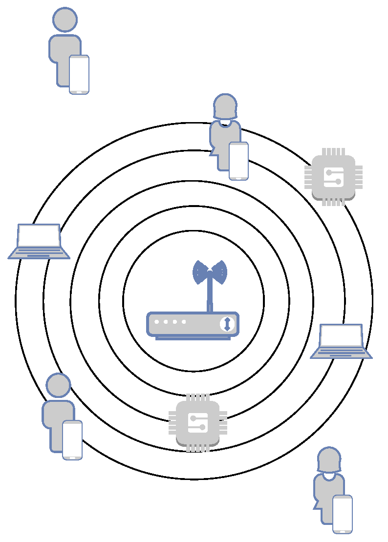
2. Edge and Dew Computing

Mobile edge computing is a paradigm that seeks to solve latency and network traffic problems found in mobile cloud computing environments [14]. Ref. [15] defines edge computing as “a model that allows a cloud-based computing capacity providing services making use of the infrastructure that is on the edge of the network”. In this way, mobile edge computing allows servers or workstations within a computer network, thus ensuring low latency while enabling the efficient processing of information, which permits the deployment of more robust applications. Furthermore, this paradigm lets edge servers work with other nodes in proximity or collaborate with cloud services, thus deploying much larger and more efficient applications [16,17]. However, while edge computing helps to reduce the network’s problems, it still depends on the network backbone that may not be available or reachable in certain situations, like working with IoT devices in mines and on ships, in deserts, or on moving vehicles.

Dew computing is a new paradigm where connected devices offload jobs to nearby devices in the same network. This paradigm proposes an architecture that reduces network latency, the energy cost of remote data communication, and the costs inherent to cloud infrastructure usage [18]. Through this, dew computing optimizes the usage of mobile and IoT devices in two manners. First, it treats mobile devices as clients in the network infrastructure to offload their work to other devices in the same network [19]. Second, dew computing considers mobile and IoT devices as resources to increase the available computational power from an existing system. In this approach, one device can offload its work onto another available device in the network (including other mobile and IoT devices) [20,21].

We note that a network topology is needed to use mobile and IoT devices as resources in a local network [3]. The Smart Cluster at the Edge (SCE) is a network topology commonly used for that purpose in dew computing. Figure 1 shows how the devices are organized in this type of network. This topology can be established wherever an access point and a group of mobile and IoT devices coexist. The topology’s main feature is a central scheduler coordinating the task assignment among the network’s available resources. This central scheduler can be any capable device in the network [22]. In this work, we address the problem of distributing jobs in a dew environment, assuming that the network topology is an SCE.

3. Related Work

Distributing jobs in dew environments optimally is a challenging combinatorial problem [6,23]. Many factors must be taken into account to assign jobs to devices correctly. Those factors range from a device’s CPU speed to a device’s availability within a time window, from how often jobs arrive at the scheduler to how urgent jobs must be completed. Many previous works have proposed heuristic methods to deal with this complex problem. A heuristic method is a practical approach to obtaining approximated yet satisfactory solutions to problems where finding the optimal solution is computationally intractable, in this case, the job assignment problem. This paper seeks human-designed heuristics that consider features from the SCE and are aware of network changes through time. Also, we explore an alternative approach, which consists of learning a policy to distribute jobs using RL. To provide a coherent view of the related work, we divided this discussion into two parts: We first discuss existing heuristic methods to distribute jobs in an SCE and then review previous works at the intersection of RL with cloud and edge computing.

In the context of SCEs, different algorithms have been proposed to optimize the system’s utility and job execution time, using the mobile devices’ remaining battery as a formal constraint of the resource allocation problem formulation [24,25,26,27,28]. These algorithms, however, assume complete and accurate information regarding the energy spent and the execution time for every candidate node, making it challenging to apply in real-life scenarios.

In refs. [29,30], they addressed the previous limitation by proposing algorithms that do not rely on complete information. This approach seeks to exploit the nodes’ proximity and cost-effectiveness of node transferring capabilities. However, their studies focused on analyzing the effect of nodes’ mobility rather than balancing the load to efficiently utilize the battery and processing power of the available resources.

Refs. [6,22] presented other types of heuristics, which distribute jobs by considering the mobile device’s battery level and computing scores obtained from benchmarks. These methods outperformed traditional scheduling algorithms (such as round robin) but have the limitation of only considering battery-dependent devices. This problem was recently addressed by ref. [7]. In ref. [7], the authors studied hybrid SCEs, which combine both battery-dependent and non-battery-dependent devices, and proposed heuristic methods that consider the device’s battery level, computing score, and current workload to distribute jobs in dew environments.

In contrast to those works, where the primary assumption was that the network topology remained static, meaning that the structure and connections within the network did not change over time, this work takes a different approach. Our research recognizes the limitations of static topologies, particularly in real-world scenarios where network environments are often dynamic and subject to change. By “dynamic environments”, we specifically refer to situations where mobile devices can enter or exit the boundary of an SCE over time, leading to fluctuations in the network’s composition and connection throughput. To address these challenges, we propose new heuristic algorithms specifically designed to adapt to network dynamic conditions. To achieve this, we improved the simulation support offered by EdgeDewSim [7], enhancing its capability to support the development of new connection-aware job distribution as the topology evolves, configure nodes’ mobility in an easy-to-reproduce manner, and represent network changes as an effect of nodes’ mobility. By incorporating these advancements, our approach aims to provide a more robust and flexible solution for job distribution in dynamic network environments.

RL Methods in Edge and Dew Computing

In cloud computing, task scheduling focuses on deciding which resources (servers) should process an incoming task. In this problem setup, previous works have shown that RL agents can reduce the execution time in distributed systems [31] and avoid overloading (and deadlocking) cloud servers [32]. Furthermore, ref. [33] showed that deep RL can help schedule tasks in large-scale cloud service providers, surpassing traditional methods in terms of energy cost and reject rates.

As for edge computing, the task scheduling problem is similar. The edge server receives tasks and has to decide whether to send those tasks to a nearby server or the cloud. Several works have explored how to distribute jobs in edge computing using deep learning techniques like convolutional neural networks or reinforcement learning according to different performance metrics. These metrics include reducing computing times [34,35], energy consumption [36], latency [37,38], task failure rate [39], or a combination of the previous [40,41,42]. We note that in edge computing, the action space is usually limited. For instance, sometimes the agent can only decide whether to send (or not) a job to the cloud [41]. In contrast, the action space in a dew environment typically ranges from tens to hundreds (i.e., one action per device), making the decision-making problem considerably harder.

RL has been increasingly utilized for job scheduling in environments that are closely related to one another, such as cloud computing [31,32,33] and edge computing [34,36,37,38,39,40,41,42]. With emerging studies in dew computing, RL has been applied in cloud and edge computing for job scheduling. For instance, in ref. [43], they propose a vehicular dew computing architecture using RL for content delivery optimization. Similarly, in ref. [44], they suggest a dew computing-based vehicular edge caching architecture to enhance vehicle stability and high-definition map acquisition. In ref. [45], they introduce dew quantum machine learning (DewQML) to improve decision making and reduce latency in dew computing environments. In ref. [46], they present a dew computing-based microservice execution (DoME) scheme using RL to minimize service delay and optimize costs in mobile edge computing.

Additionally, research shows deep RL agents can effectively offload jobs in dew computing environments. Finally, in the context of job offloading in dew computing environments, prior research demonstrates that deep RL agents can offload jobs more effectively than traditional state-of-the-art heuristic methods, even when faced with previously unseen scenarios. The study conducted by [9] empirically proves that the agent learns to generalize in network environments that lack dynamic components when continuously exposed to new situations. This means that the agent can appropriately distribute sequences of jobs that arrive in patterns and sizes not encountered during training. Furthermore, the agent can learn to effectively distribute jobs in fixed dew environments, significantly outperforming state-of-the-art heuristics regarding the number of instructions executed per second. This highlights the potential of RL in enhancing the efficiency and adaptability of job scheduling in dew computing environments, paving the way for more responsive and robust computing systems [9].

In the same line of ref. [9], there are three main differences between our work and the existing work on RL with cloud and edge computing. We address a different problem. Distributing jobs in a dew environment has challenges that do not typically arise in cloud or edge computing. For instance, in dew computing, some devices might run out of battery, or users might start interacting with them. When the network conditions are dynamic, the availability of the devices cannot be assured. Taking these elements into account is a nontrivial task. Second, we thoroughly examine the transfer learning capabilities exhibited by the policies acquired by the reinforcement learning agent. This is a crucial step toward applying RL methods in natural systems since, in practice, it is unlikely that the agent would encounter scenarios that it had previously seen during the training. Finally, we use an RL agent better suited for generalization than the agents used in previous works [47,48].

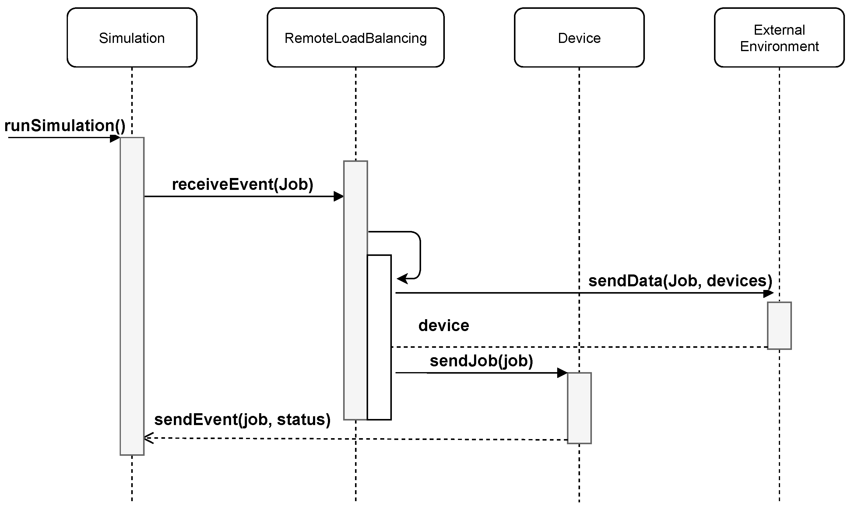
4. EdgeDewSim Extended Simulator

The EdgeDewSim Simulator [7] was built as an extended version of DewSim [49], in which new features were added. It incorporates the notion of worker nodes that do not depend on batteries to cooperate in job execution, i.e., edge nodes without energy constraints. In the present work, we extended EdgeDewSim with the functionality to model the effect of node mobility on connectivity status. We will refer to the latter extension, i.e., EdgeDewSim, which has mobility functionality, as the EdgeDewSim Extended Simulator.

The previous version of the EdgeDewSim Simulator [7,9] did not have support for allowing devices to connect and disconnect from the network; because of this, the first task of this work was to extend the EdgeDewSim Simulator to include this new feature. The extended simulator version allows researchers to provide a connection file, in the form of a trace, for each device containing all the connection and disconnection events the device will go through during the simulation. The connection file provided to the simulator uses the following syntax:

# Connection Event; Event Time (ms)

ENTER_NETWORK;1000

LEAVE_NETWORK;2000

where the field before the semicolon indicates the device status for the SCE, and the field after the semicolon refers to the time (expressed in milliseconds) when the status change event will occur. Such a time is always relative to the time zero of the simulation. More explicitly, a device configured with the connection file given in the example will join the SCE a second after the simulation starts and leave the SCE two seconds after the simulation begins, providing a permanence time of one second within the SCE.

In the EdgeDewSim Simulator [7], devices were configured to connect to the network as soon as the simulation started, and there were no events related to device disconnection due to mobility. Instead, devices would only disconnect from the cluster when their battery was depleted. This behavior was implemented through a series of events, including device joining, device leaving, and state of battery updates, to which a scheduler entity would subscribe to maintain an up-to-date list of candidate devices for executing jobs.

Two main features must be addressed to accommodate device connection and disconnection due to mobility. Firstly, devices should be able to discharge their battery even when they are not part of the cluster or network. This adds a layer of realism to the simulation, reflecting the natural battery consumption of mobile devices in real-world scenarios. Secondly, the schedulers require a memory mechanism to keep track of potential devices that can execute a job every time they connect to the network. This memory should also be updated to remove devices from the list whenever they disconnect from the network. This feature is crucial for efficiently managing the dynamic nature of mobile device clusters, as it ensures that the scheduler has an accurate pool of devices to choose from for job execution.

The EdgeDewSim Extended Simulator incorporates the above-mentioned features and offers backward compatibility for conducting experiments before implementing these features. This is achieved by using connection files in which devices are set to connect at the start of the simulation and remain connected throughout without any disconnection events caused by mobility. This simplifies the simulation environment and allows for testing other aspects of the system without the added complexity of the device mobility feature. However, incorporating the above-mentioned features is essential for a more comprehensive and realistic simulation of mobile device clusters.

4.1. Device Connection Score

The scheduler must determine which device is more suitable for executing a job. To start considering the connection and disconnection, it is necessary to add logic to the device to report a connection score as a heartbeat. This concept will be explained in more detail in Section 6; nevertheless, it is relevant to know that other authors [50] have used WiFi to predict the length of a connection to an access point, geo-located tags [51] to indicate the following location of the device, and other sources of data from the device such as battery state, WiFi signal strength, and GPS traces, among others.

4.2. Device Connection Event

To address this issue, certain events were modified, and new ones were created. The event type $DEVICE\text{\_}START$ was modified to solely initiate CPU usage and battery discharge of the device upon joining an SCE. Before the modification, such an event causes the device to be added to the scheduler’s list, and the device’s state is reported to the scheduler. With the modification, two new event types were introduced. The $DEVICE\text{\_}CONNECT$ event now manages the actions previously performed with a $DEVICE\text{\_}START$ event and updates the connection score from Section 4.1.

4.3. Device Disconnection Event

The event $DEVICE\text{\_}DISCONNECT$ removes the device from the scheduler’s list of possible devices that can execute jobs. Also, the device stops sending the scheduler updates of its battery state of charge. The $DEVICE\text{\_}DISCONNECT$ also needs to handle what happens to the jobs being executed by the device at the moment of disconnection and the ones that are queued for future execution; in this implementation, these jobs are canceled when the device disconnects from the network. This could be improved or changed in future work to simulate that jobs are executed in the background and results are cached and sent once the connection is reestablished; it all depends on the scenario being tested. Regarding the network model, this had to be modified to accept the disconnection of devices and be able to cancel the transfer of messages related to the device disconnecting from the network.

5. Human Mobility Modeling

Humans constantly move to our jobs, universities, schools, or any other destination daily. However, this behavior is nothing new; throughout history, humans have migrated between different territories countless times, as mentioned in ref. [52]. A significant change between a few decades ago and now is the high usage of smart devices within the population; this growth in usage is mainly due to the high adoption of smartphones in our lives [53,54].

This characteristic of the current state in the adoption of smartphones has attracted the interest of scientists in researching human mobility, mainly because now we have the tools to collect accurate data that can help to create models that can mimic our mobility patterns. Nowadays, there are multiple ways to obtain data from human mobility. GPS traces are one of these sources for mobility patterns. Also, CDRs (called detail records) have been used to learn from human mobility, and, finally, from some datasets of connection to an access point like a WiFi [55,56] point. In this field of research, although there has been significant progress in terms of data sources, the use of synthetic data from mobility models continues to be prevalent. This is because synthetic data remain a convenient method for studying and proposing new mobility models.

As mentioned in ref. [57], we can divide human mobility models into nonsocial, social, and hybrid categories. Others [53] divide them into movement-based, linked-based, and network-based. Individual or movement-based mobility models are generated from individual traces of either GPS, CDR, or any other data source that can describe how a human moves without the influence of other humans over his or her patterns. On the other hand, social, network-based, or linked-based models try to model human mobility patterns, considering the different interactions we, as humans, have and how these social interactions can affect our mobility patterns [53]. In this work, we will focus on individual or movement-based mobility models, notably random walk and random waypoint, to generate the connection and disconnection events from an access point. We mainly chose these two models to generate synthetic data because they represent the most dynamic scenarios, since nodes tend to move randomly. This way, we could expose our proposed human-designed heuristics (RelBPA, ReleSEAS) and the RL agent to hostile environments. To develop these data, we used PyMobility [58] as a base for the mobility algorithms and added a layer of code to check the connections and disconnections from the devices. Then, these data were used as input for the EdgeDewSim Extended Simulator.

5.1. Random Walk

Random walk is the most simple mobility algorithm [57], where an individual’s movements are simulated by a statistical model, which sets an individual in a particular scenario defined by its minimum and maximum displacement velocity and the rotation angle. This algorithm randomly chooses the individual’s velocity at each step and the direction, which can be in the range of $(0,2\pi )$; this process repeats at every simulation step. This model is the most basic one because it is far from representing realistic human movements that are not random at all.

5.2. Random Waypoint

Random waypoint is a variation of the previous model [57,59], with the difference that now an individual moves to a waypoint where it waits a certain amount of time until it can choose randomly its speed and direction.

6. Connection-Aware Scheduling Heuristics

This paper proposes two new scheduling heuristics, ReleSEAS and RelBPA, based on previously developed heuristics, E-SEAS and BPA.

6.1. Reliability Score

To ensure that the stability of the devices in the network is considered, we suggest introducing a new score that the heuristics should consider. This score, similar to the battery level, aims to influence the decision-making process used by the heuristic. We refer to this score as the “reliability score”, denoted by $Reliability$. It is calculated as follows:

$$Reliability=\left\{\begin{array}{cc}curr\text{\_}execution\text{\_}time\hfill & \mathrm{if}not first\text{\_}disconnection\hfill \\ avg\text{\_}connection\text{\_}time\hfill & \mathrm{otherwise}\hfill \end{array}\right.$$

(1)

where $first\text{\_}disconnection$ is a variable that each device has to express if it has disconnected from the network for the first time; the variable $curr\text{\_}execution\text{\_}time$ represents the amount of time in milliseconds executed since the start of the execution to the time the $Reliability$ score is calculated; and finally, $avg\text{\_}connection\text{\_}time$ corresponds to the average time that the device has been connected to the network, taking into consideration these connection events can happen multiple times over a simulation and that the metric is calculated only for the devices connected to the network.

The following example demonstrates the calculation of the reliability score. In a hypothetical case, we have two devices. The first one has the subsequent connection and disconnection events: $t=1$ (connect), $t=2$ (disconnect), $t=5$ (connect), $t=10$ (disconnect). The second device connects at $t=0$ and disconnects at $t=10$. Assuming the simulation clock is at $t=11$, the reliability score for the first device will be $3=(1+5)/2$ and 10 for the second device. In this example, we can see what the reliability score aims to incorporate as new information about how stable a device is for the time it plays the role of a worker node within a cluster. The proxy calculates the reliability score when a job arrives and needs to be distributed; in this way, it can obtain the ranking for each device. Also, every time a device disconnects, its last connection duration is stored to be used for the following calculation of the reliability score.

6.2. ReleSEAS

The main feature of E-SEAS [6] is that it is easy to implement in real-life environments because it requires easy-to-obtain information, such as battery level, nodes’ computing capability measured in FLOPs (float point operations per second), and remaining jobs as nJobs to build a rank of devices joined to the cluster. Then, the E-SEAS ranking formula is defined as follows:   

$$E-SEAS=\frac{flops·SOC}{nJobs}$$

(2)

A scheduler applying E-SEAS criteria assigns jobs using this ranking. Every incoming job triggers a recalculation of the ranking, which uses fresh information about jobs’ and nodes’ statuses, such as job queue size and battery level at each node. Job counters and node status records are maintained by a centralized component called the proxy, from where the scheduler operates. This component keeps track of all information necessary to recalculate the ranking. In this paper, we propose incorporating a new score (reliability score) into the E-SEAS ranking formula to boost the ranking of devices connected to the network for extended periods. This modification derives into what we call ReleSEAS:

$$ReleSEAS=\frac{flops·SOC·Reliability}{nJobs}$$

(3)

where $flops$ is the device capabilities (processor speed) measured in float point operations per second, $SOC$ is the last report of the state of charge (battery level), and the reliability is calculated using Equation (1).

6.3. RelBPA

BPA [7] is a scheduling algorithm that considers the jobs loaded onto devices and the present hardware capabilities to select the best device to execute an incoming task. The ranking formula for BPA is defined as follows:

$$BPA=\frac{\Sigma OP\text{\_}jobs}{flops·Battery}$$

(4)

where $OP\text{\_}jobs$ is the current job load in a device’s queued jobs in terms of how many operations are needed to finish those jobs; $flops$ is the device capability (processor speed) measured in floating-point operations per second; and $Battery$ is the remaining battery of the device expressed in values between the range of $0<Battery\le 1$ [7].

The reliability batch processing algorithm (RelBPA) is an adaptation of BPA that incorporates the reliability score introduced in Section 6.1. In the same way as ReleSEAS, the purpose of adding the reliability score is to boost devices that have been connected to the network for more extended periods; the reliability score is added to the denominator to make the metric as small as possible. The ranking formula for RelBPA is defined as follows:

$$RelBPA=\frac{\Sigma OP\text{\_}jobs}{flops·Battery·Reliability}$$

(5)

where the variables used in the formula have the same meaning as in BPA, and the reliability score is calculated using Equation (1).

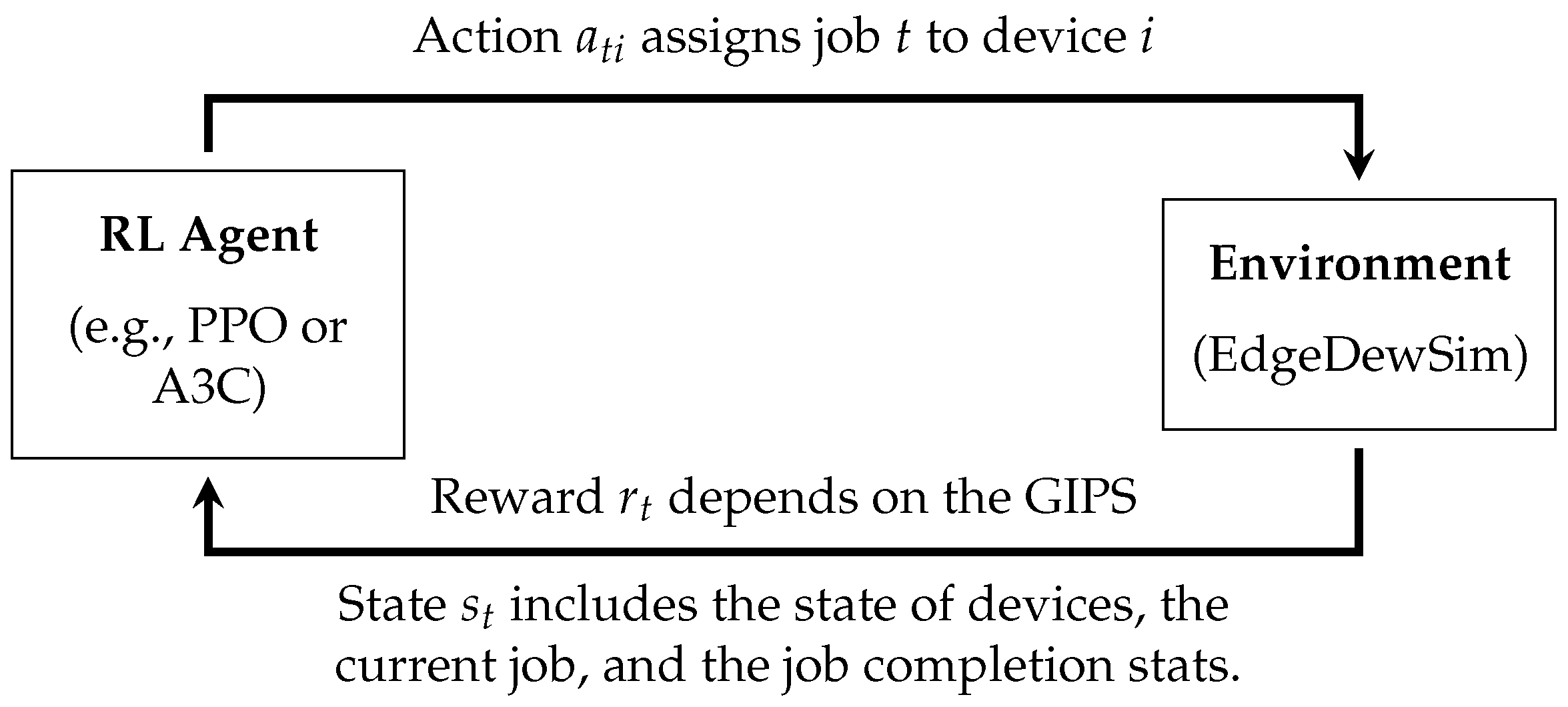
6.4. Connection-Aware Reinforcement Learning Agent

In this section, we discuss how we integrate dew computing with RL. First, we formally define the problem of job scheduling in a dew environment. Then, we describe how to solve such a problem using RL. Finally, we discuss the software architecture behind our proposed solution, combining the EdgeDewSim Extended Simulator with the RL framework OpenAI Gym v0.21.0 [60]. But first, we briefly discuss the notation that we use in this section.

6.4.1. Notation

Below, we use the following notation. We use uppercase letters to refer to sets of elements and lowercase letters to refer to individual elements in those sets. For instance, we use J to denote the possible jobs that arrive in the dew environment and $j\in J$ to indicate one particular job in J. In addition, $\left|J\right|$ denotes the number of elements in J. Elements in a set have different features. To refer to the value of a feature, we use $x.feature$. For instance, $j.\mathrm{ops}$ refers to the number of giga-operations of job $j\in J$.

6.4.2. Problem Definition: Job Scheduling in Dew Computing

We tackle the problem of distributing jobs in a dew environment. The dew environment consists of devices connected to a local network. Some of these devices can be IoT devices that have an unlimited power supply (e.g., Raspberry Pis and personal computers), and others are mobile devices with a limited battery (e.g., tablets and smartphones). In addition, one node in the local network is assigned as the scheduler. The scheduler’s purpose is to receive and distribute jobs among the devices.

Once a job is assigned to a device, the time it takes to complete (and how much battery it consumes) depends on the job’s features and the device’s current state. For instance, since some devices have limited battery life, a job might not be completed if assigned to a device with a low battery level. Users might also interact with the devices, and the local network might have congestion issues. The scheduler must consider all these factors to distribute jobs effectively.

In more detail, assigning a job to a device adds that job to the device’s job queue. Then, the device will keep running the jobs in its queue, one by one, until they are completed or running out of battery. Once a device runs out of battery, all the jobs in its current queue are discarded. If a job is assigned to a device that has no battery, that job is also discarded. In our experiments, a job is not reassigned to a different device when the job is discarded. This forces the scheduler to be extra careful when assigning a job to a battery-dependent device.

To evaluate the effectiveness of a given job distribution, we use the giga-instructions per second (GIPS) that are completed in the dew environment:

$$\mathrm{GIPS}(t_0,t)=\frac{{\sum }_{j\in J_c}j.\mathrm{ops}}{t-t_0},$$

(6)

where $J_c\subseteq J$ is the subset of jobs that were completed within the time interval $[t_0,t]$ and $j.\mathrm{ops}$ is the number of giga-operations of job $j\in J_c$. Intuitively, GIPS measures how many operations are completed in a unit of time. The scheduler aims to distribute the jobs to maximize the GIPS in the dew environment.

In this study, we postulate that the dew computing environment is subject to a limitation regarding the maximum number of devices that can be integrated into the network at various intervals. This constraint results from the restrictions imposed by the size of the RL model, which is crucial for optimizing network performance and decision making and cannot accommodate an undefined number of devices. Understanding the implications of this restriction is essential for managing the network’s scalability and ensuring that the dew environment can efficiently handle the dynamic addition of devices over time.

6.4.3. Environment Definition: States, Actions, and Rewards

The first step in applying RL in dew computing is to define the environment in which the agent will interact adequately, that is, to define the states S of the environment, the actions A that the agent can perform, and the reward signal $r(s,a,s^{\prime })$ that the agent will optimize for. We also have to define the transition probabilities $p\left(s^{\prime }\right|s,a)$ if the agent does not interact with a real system (or with a predefined simulator). Whether the agent succeeds or fails at distributing jobs in a dew environment partially depends on how we define those four elements: S, A, r, and p.

To define a dew environment in terms of S, A, r, and p, our starting point was EdgeDewSim Extended Simulator. As presented in Section 4, EdgeDewSim Extended Simulator inherits the simulation features of DewSim and EdgeDewSim, including the energy consumption of each device, battery-dependent and non-battery-dependent devices as contributors of an SCE, the job executions, and user behaviors, and, in this work, it incorporates features to represents network status changes due to nodes’ mobility. Thus, the transition probabilities p in the environment are modeled by EdgeDewSim Extended Simulator.

To define the state space S, we considered two critical features of RL. First, most RL agents do not have memory. They learn a policy $\pi \left(a_t\right|s_t)$ that makes decisions purely based on the information available in the current state $s_t\in S$. Thus, $s_t$ must include all the relevant information the agent needs to assign a job to the correct device. Second, we note that any information identical for all the states $s\in S$ is useless for the agent. The reason is that the agent has to discriminate whether action a is a good action in state s. If a subset of information $x\subset s$ is identical for all states, then x provides no discriminatory information to the agent.

We then define the state space as follows: $S=D\times J\times C$, where $(d,j,c)\in S$. Specifically, $d\in D$ contains information on the current state of each device. This information includes, for each device, its CPU usage percentage, its remaining battery, the network strength, the connection status, and its current job queue. Then, $j\in J$ provides information about the job the scheduler must assign next. This information includes the job’s ops, input size, and output size. Finally, $c\in C$ contains general statistics about the previously completed jobs. These statistics include the number of jobs that have arrived, the number of jobs that have been completed, the sum of the jobs’ ops that have been completed, and the elapsed time since the beginning of the simulation (i.e., $t-t_0$). We note that $s\in S$ comprises all the necessary information to correctly assign job j to a device in a fixed dew environment. If the environment is not fixed, we might want to add some additional features, such as the number of instructions per second a device can execute (or its battery capacity). We discuss this further in Section 8.

Our definition of the action space A is as expected. We define one possible action per device in the dew environment. Then, whenever the agent executes action $a_i\in A$ given the current state $(d,j,c)\in S$, the job j is assigned to the device associated with action $a_i$.

Finally, the reward function is equal to the number of successful jobs executed in the dew environment, as defined in Equation (6). Formally,

$$r(s,a,s^{\prime })=\left\{\begin{array}{cc}\frac{|J_c|}{\left|J\right|}\hfill & \mathrm{if}{s}^{\prime }\mathrm{is}\mathrm{terminal}\hfill \\ 0\hfill & \mathrm{otherwise}\hfill \end{array}\right.$$

(7)

Note that this reward function only rewards the agent in terminal states. After the agent finishes distributing the whole sequence of jobs, the agent receives a reward equivalent to the successfully executed jobs in the dew environment. As a result, any optimal policy ${\pi }^{*}\left(a\right|s)$ will optimally distribute jobs according to our problem definition from Section 6.4.2.

As a summary of this section, Figure 2 illustrates the training loop and how a learning agent interacts with our proposed environment. The agent assigns the current job to a particular device using its actions. In response, the dew environment returns the next state $s_t$ and a reward $r_t$. The state includes information about the current job to be assigned and the state of the devices. The reward $r_t$ will be zero unless the agent has just distributed the last job. If that is the case, $r_t$ will be equivalent to the successfully executed jobs. Since the agent tries to maximize the reward received from the environment, it will learn to distribute jobs to improve the performance of the dew environment.

6.4.4. Implementation Details

For the dew environment simulator, we used EdgeDewSim Extended Simulator. This version can handle both battery-dependent and non-battery-dependent devices. To simplify the process of training and testing deep RL methods, we also developed an OpenAI Gym environment [60]. This allowed us to quickly and easily test different RL agents using existing implementations made for the OpenAI Gym library.

Since EdgeDewSim Extended Simulator is written in java and OpenAI Gym is written in python, we developed an interface that allowed us to control EdgeDewSim Extended Simulator from OpenAI Gym. To do so, we added logic on top of EdgeDewSim Extended Simulator to delegate the scheduling decision to an external agent so that every time a job arrives, the simulator broadcasts the general state of the simulation and then listens for which device has to be selected, as shown in Figure 3. Then, we developed a new RL environment, following the guidelines from OpenAI Gym [60], that undertakes three main things: (i) it establishes the connection with the simulator, (ii) it sends actions to the simulator, and (iii) it resets the environment to restart from an initial state. Further details about our implementation can be found in Section 4.

7. Methodology and Experimentation

7.1. Methodology

The experimental design utilized in this study can be categorized into two main groups. The initial group focused solely on human-designed heuristics. It aimed to evaluate the effectiveness of the proposed heuristics, specifically ReleSEAS and RelBPA, in comparison to random device selection and previously examined heuristics, namely, eSEAS and BPA, as elaborated in Section 7.2. The second group was devoted to substantiating the capacity of a reinforcement learning agent to emulate the performance of human-designed heuristics. Furthermore, it sought to demonstrate the agent’s adaptability to novel conditions by utilizing transfer learning techniques; this will be explained in depth in Section 7.3.

7.2. Human-Designed Heuristics

The method employed for the assessment of human-designed heuristics comprised two sequential stages. The initial step involved generating connection and disconnection events for individual devices, while the subsequent stage entailed the execution of simulations utilizing the EdgeDewSim Extended Simulator.

As mentioned in Section 5, we employed random walk and random waypoint models to generate synthetic data for our experimental work. For each distinct human mobility scenario, we introduced variations generated randomly using a variation of generation of some parameters of these models (like speed, initial position, connection, and disconnection events). This approach yielded a range of scenarios representing diverse conditions for device mobility within the network context.

We performed 20 simulation runs for each model with unique parameter settings that affect human movement patterns. Despite the variations, certain fundamental elements remained unchanged in both models. These constants encompassed a 60 m by 60 m grid defining device movement, a consistent use of 25 devices, and a centrally located Wi-Fi access point covering a 30 m radius. Given the reliance of these models on random variables, we conducted 10 sets of 20 simulations to obtain an average value for job completion and performance. The objective behind using this number of sets is to have multiple cases using the mobility models to generate data by adjusting the parameters so the heuristics and the RL agent can interact with multiple different scenarios.

7.3. Reinforcement Learning Agent

The training method used for the RL agent was divided into two phases. The first was to train an agent using a set randomly selected from 20 random walk environments. A different selection was made for each iteration in the training phase. The environments were the same used in Section 5, each composed of 25 devices, a 60 m by 60 m grid with centrally located Wi-Fi access covering a 30 m radius. The Job J set contains jobs with [15–25] Kb data input and [1–2] Kb data output and computing requirements in the range of [80–125] mega float-point operations.

For the RL agent, we used a convolutional neural network (CNN) with five layers of 512 neurons, based on previous experience [9] where this architecture demonstrated a good balance between computational efficiency and learning capacity. The learning rate was set to $1\times {10}^{-5}$, chosen to ensure a stable and gradual learning progress. We utilized 32 Gym environments to parallel and speed up the training process. The lambda and gamma functions were both set to $1.0$ to give equal importance to all states in the value function estimation. The model was trained for $5\times {10}^7$ steps with a batch size of 64, which were determined through experimental tuning to optimize the trade-off between training time and model performance.

The other phase was related to the transfer learning phase due to the high probability of overfitting in RL [61,62]. We trained a new environment using the previous model as a base, and with fewer steps, we achieved convergence in the new environment. We repeated these steps with different environments and collected the data. The new random waypoint environments with 25 devices and 1500 JOBs were new. We trained the latest models in $1\times {10}^6$ steps and a batch size of 64.

7.4. Experimentation

This section aims to summarize the results obtained from the experiments defined in the previous section, which will be separated into two subsections. In conformity with [7], the most relevant metrics to review are the job completion rate and the executed operations at the SCE level, i.e., considering that an SCE, as a virtual processing node, renders execution services to an external entity through the devices integrating it. As mentioned in Section 7.2, we have 200 instances by model and set of jobs, with 800 experimentation scenarios. The experiment results are presented in the following subsection, and in Section 7.6 they will be further analyzed. Due to resource computing limitations, we could not fully simulate a video stream on the RL agent. We made a sample of 1500 jobs to train the agent to have representative results. On the other hand, the human-designed heuristics do not require heavy computation resources, so we ran experiments with the 1500 jobs sample and the complete set of 36,000 jobs.

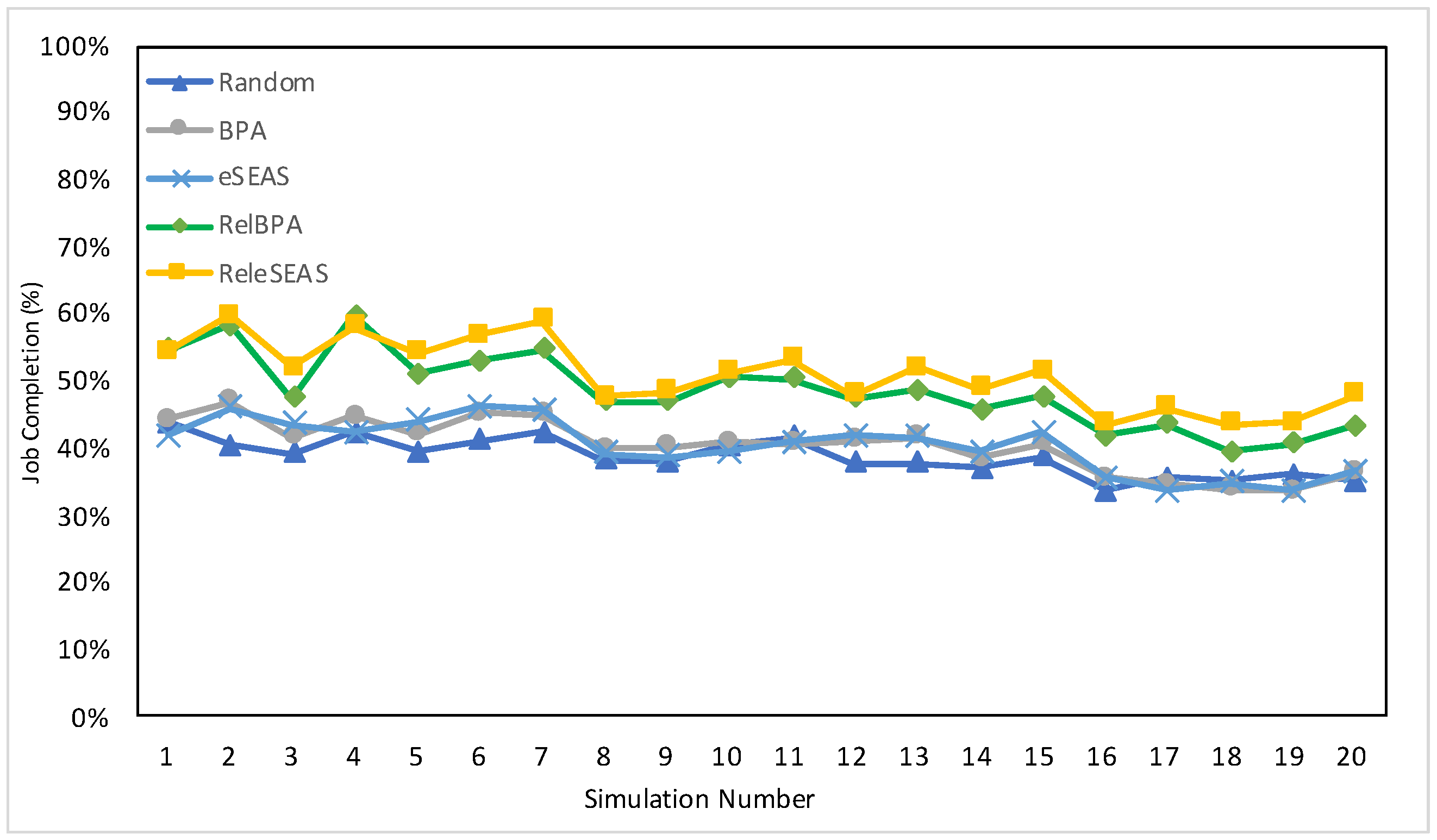
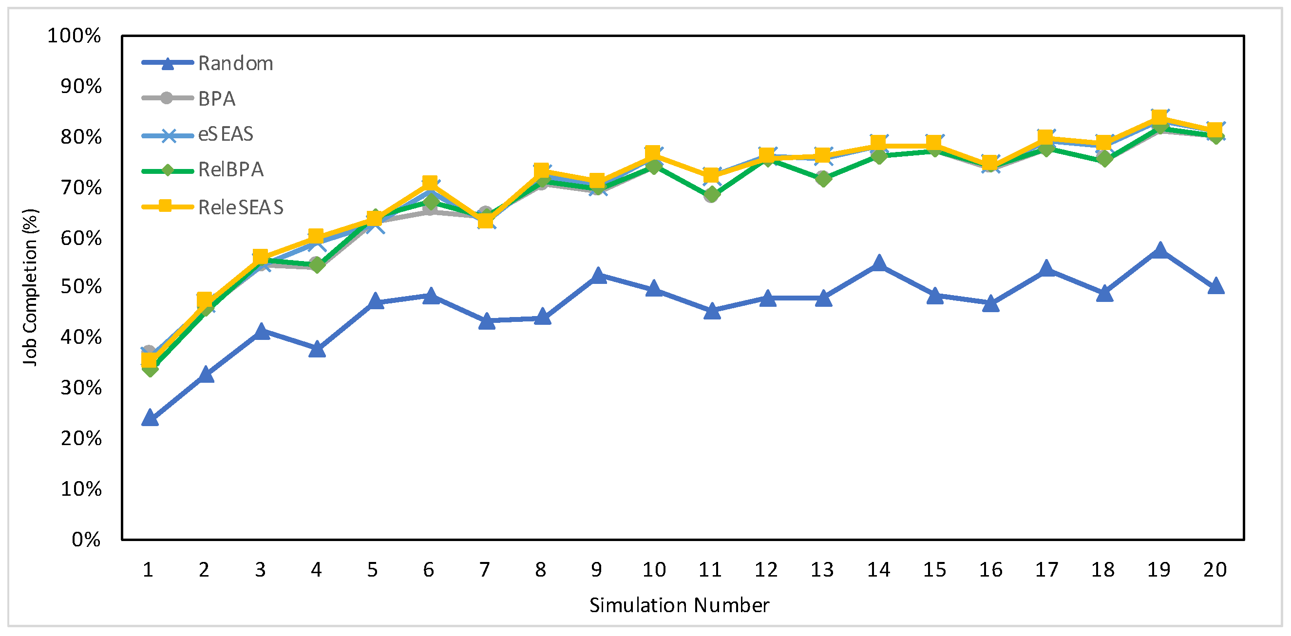
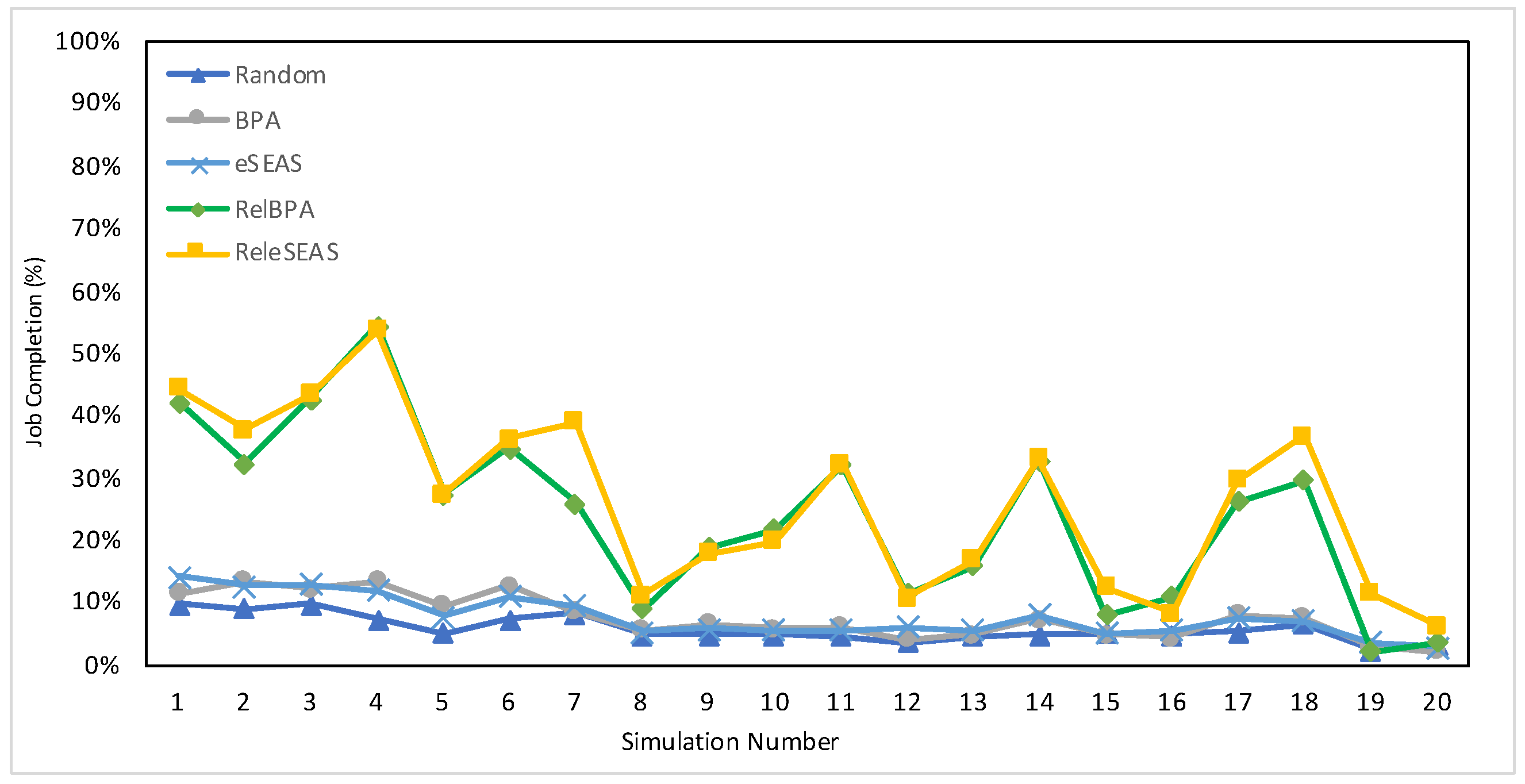
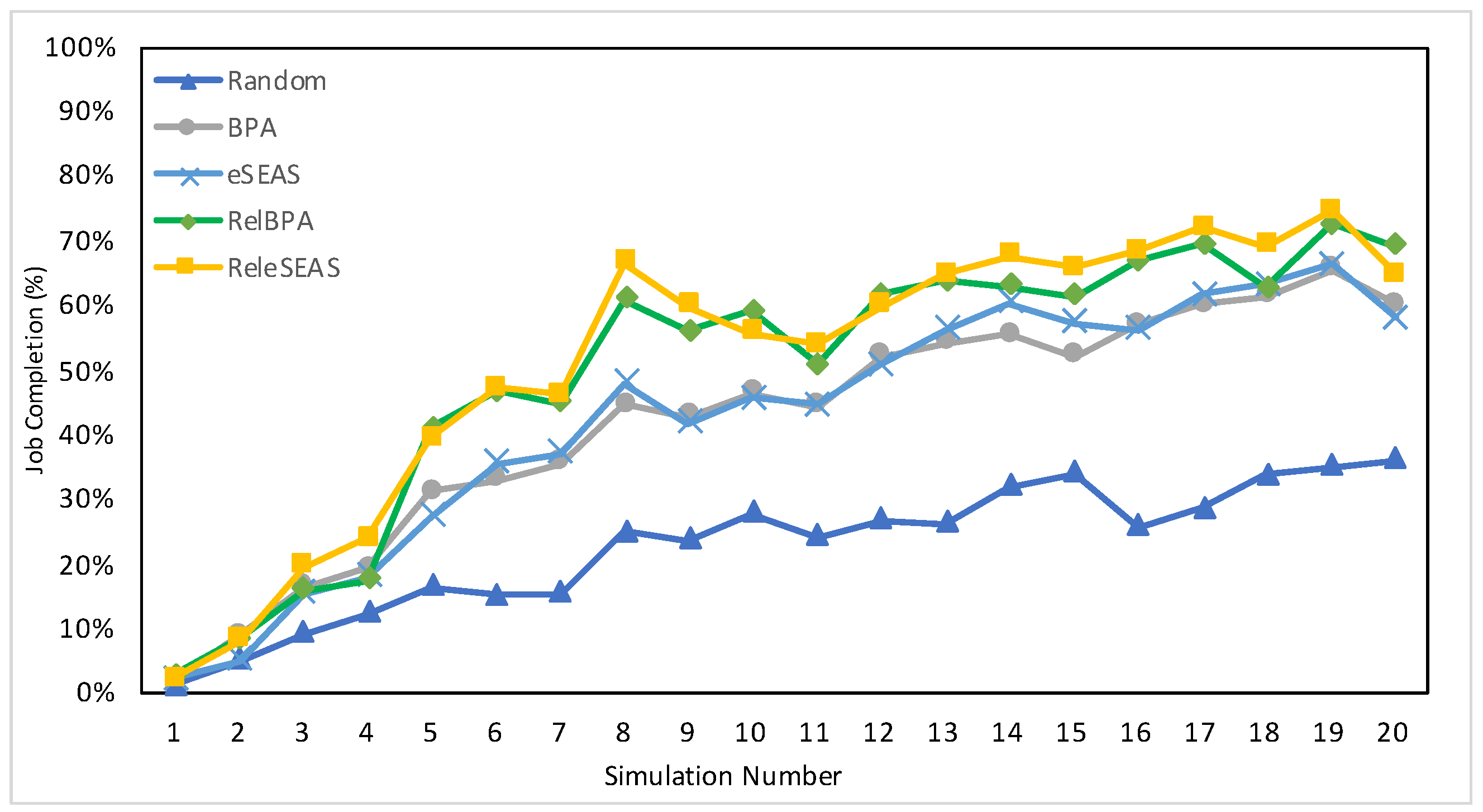
7.4.1. Job Completion

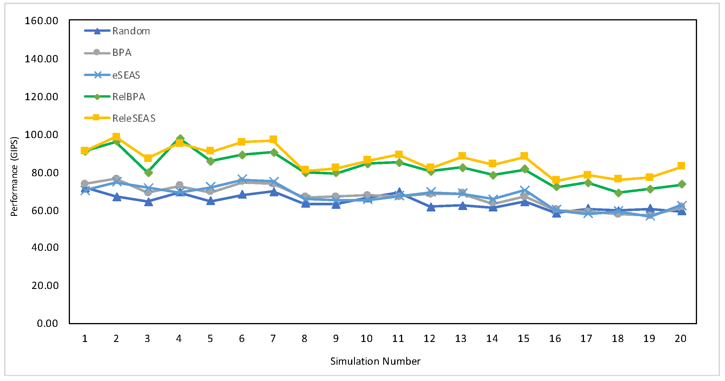
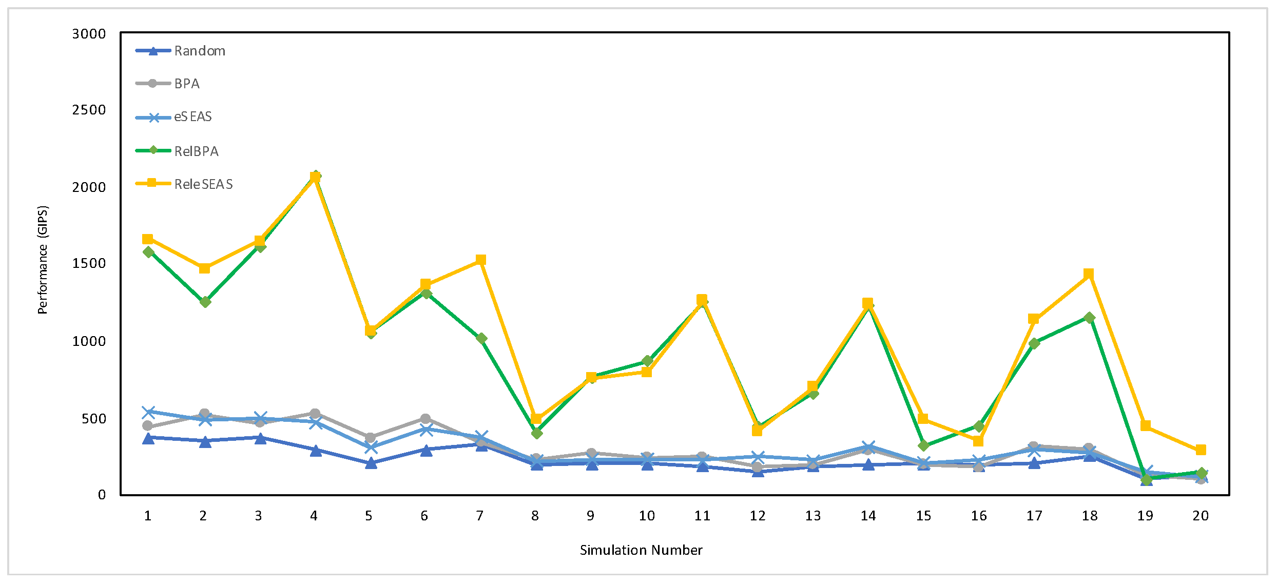
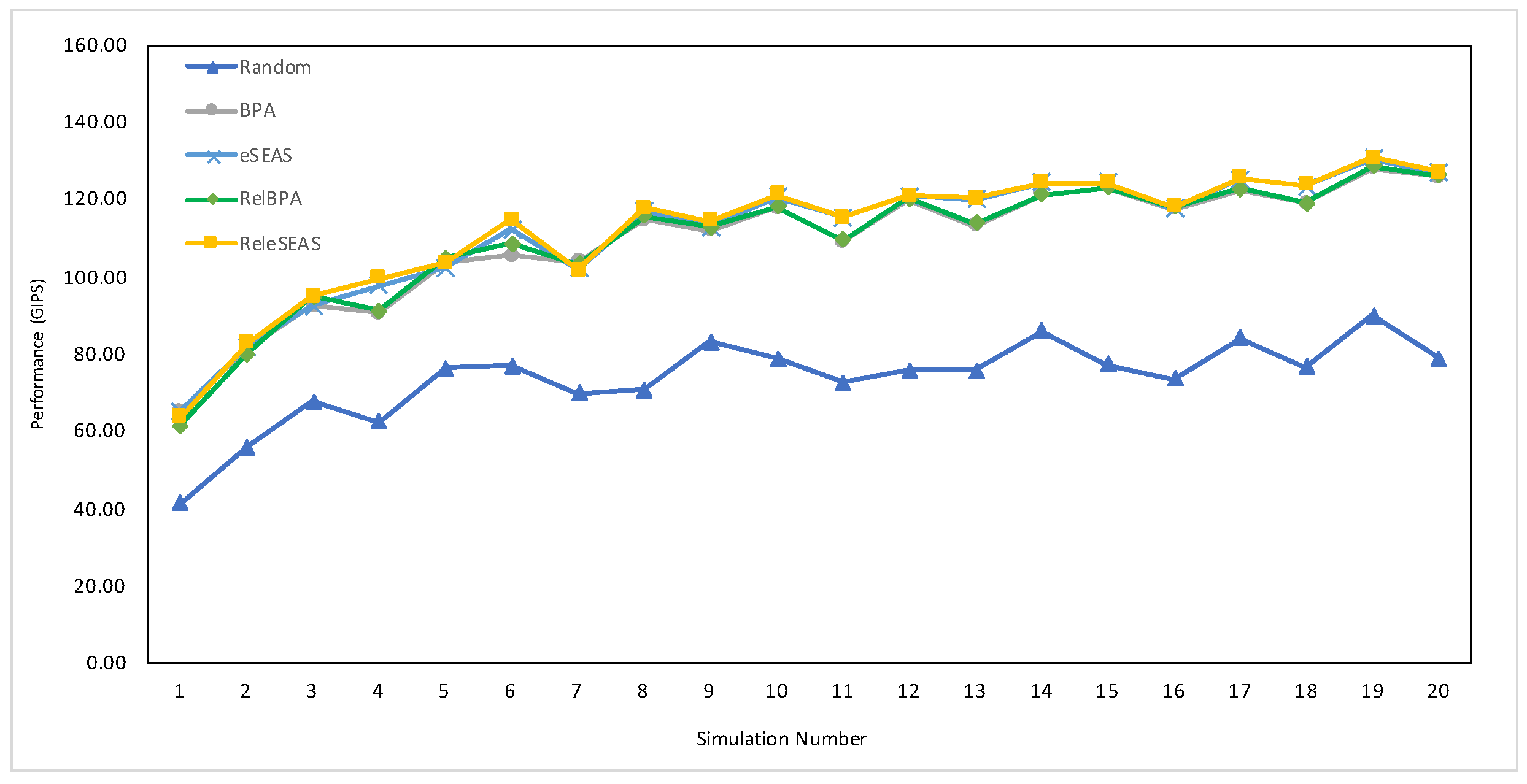
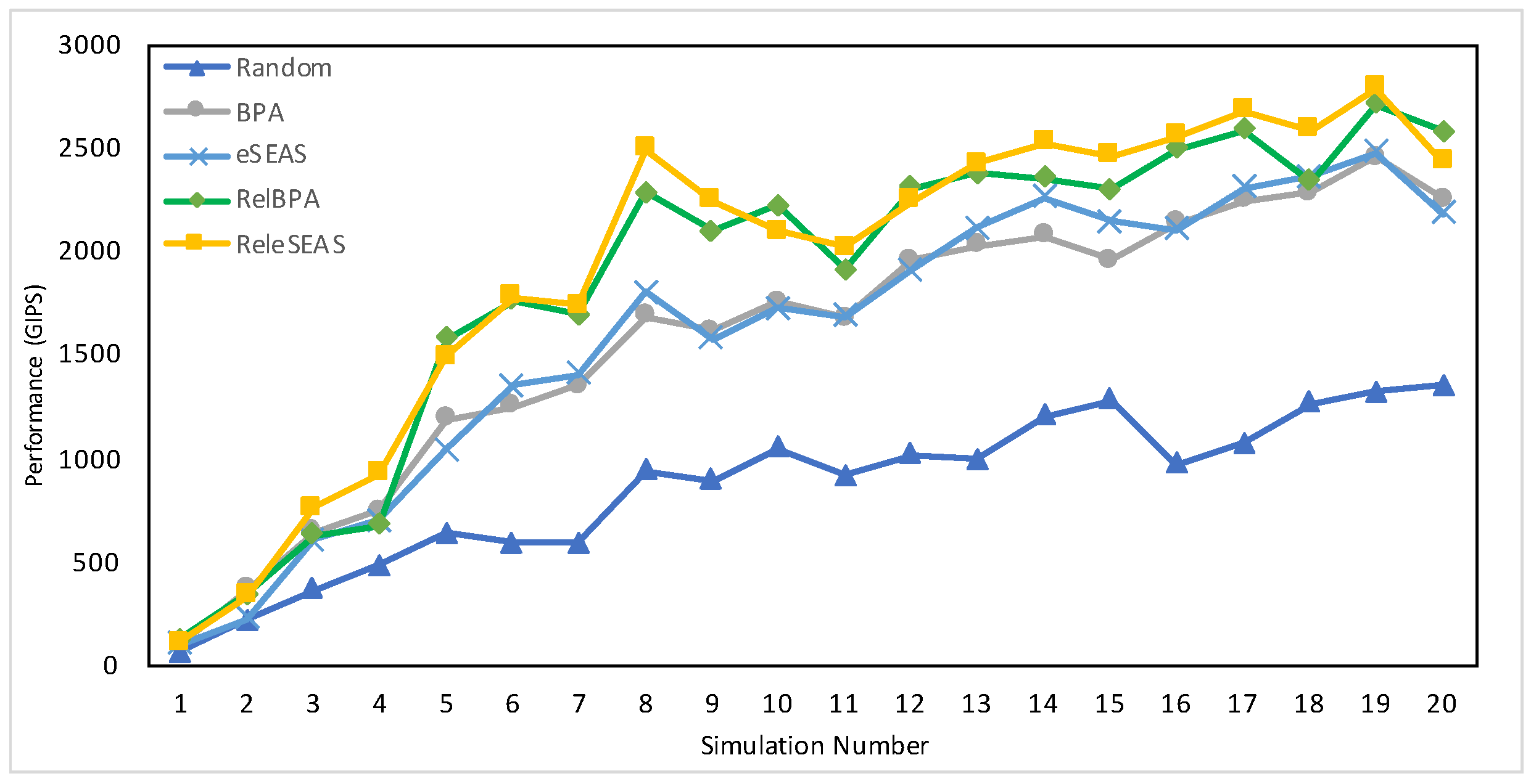
This section is divided into two parts: the results regarding human-designed heuristics and those obtained by the RL agent. In Figure 4, we present the average from 20 simulations when using random walk along with the 1500 jobs set; analogously, the same results are given when using random waypoint in Figure 5. In Figure 6 and Figure 7, we present the same 20 simulations but using the entire dataset of jobs.

As mentioned previously, we performed experiments on two different sets of jobs. The primary goal of the comprehensive dataset of jobs is to highlight that when the simulation runs longer and thus encompasses more events, the proposed human-designed heuristics demonstrate improved performance compared to their original counterparts. The results shown in

Table 1. Average job completion throughout all simulations using random walk.

Job Set	Random	BPA	eSEAS	RelBPA	ReleSEAS
1500	38.69%	40.38%	40.40%	48.59%	50.98%
36,000 (full set)	5.75%	7.56%	7.63%	24.05%	26.39%

are proof of this since in the set with 1500 jobs, the original human-designed heuristics do not deviate too much from the new variation we present in this paper. For instance, the difference in job completion between BPA and RelBPA is 8.21%, whereas between eSEAS and ReleSEAS it is 10.58%. On the other hand, when using the complete set with 36,000 jobs, the difference between BPA and RelBPA increases to 16.49%, then again for eSEAS and ReleSEAS, the difference rises to 18.83%. In both cases, the difference in job completion between the original human-crafted policy and the new version almost doubles when using the complete set of jobs over the small set. This same behavior can be seen in

Table 2. Average job completion throughout all simulations using random waypoint.

Job Set	Random	BPA	eSEAS	RelBPA	ReleSEAS
1500	45.97%	67.58%	69.17%	67.75%	69.51%
36,000 (full set)	22.74%	42.21%	42.60%	49.73%	51.52%

, in which the usage of Random Waypoint makes this difference smaller than the results obtained using Random Walk. An additional Random scheduler is added to these results to use as a baseline, which distributes the jobs randomly every time the given event is received.

7.4.2. Performance

As in Section 7.4.1, the current section is also divided into two subsections, one regarding human-designed heuristics results and the other for the RL agent. In Figure 8 and Figure 9, we present the performance measured in GIPS for each human-designed heuristic using random walk as the model to generate connection events for 20 simulations. As seen in Figure 8, the values obtained for each simulation across all heuristics are not spread out but are instead close, which translates to small differences between the proposed heuristics with the reliability score and those that do not have the score. On the other hand, Figure 9 shows a different scenario where ReleSEAS and RelBPA can separate from the competitors in a significant way in most cases. In Figure 10 and Figure 11, which present the performance when using random waypoint, we can see the same behavior but with less strength.

In this metric, we use the complete and small datasets to explore whether the same relation is in job completion. Even though both metrics are highly related, having more completed jobs does not necessarily mean that the performance in GIPS will be equally high. This is because modeled jobs can—as in real life—be simple or complex; we might want to process a simple math calculation or run an image through an object detection model. Nevertheless, the exact relationship between the original human-designed heuristics and the proposed versions remains for both metrics.

In Figure 8, the values obtained for each simulation across all heuristics are not scattered but are instead close, which translates to slight differences between ReleSEAS and RelBPA with regard to the original versions. On the other hand, Figure 9 shows a different scenario where ReleSEAS and RelBPA can significantly separate from the rest of the policies when using the complete set of jobs. In regard to the performance metric, we can see in

Table 3. Average performance in GIPS across all simulations using random walk.

Job Set	Random	BPA	eSEAS	RelBPA	ReleSEAS
1500	64.36	67.05	67.18	82.03	86.25
36,000 (full set)	231.69	303.27	305.30	935.17	1029.76

a difference of 14.98 GIPS for BPA and RelBPA, whereas for eSEAS and ReleSEAS, the difference is 19.07 GIPS. On the other hand, when using the complete set of jobs, the difference between BPA and RelBPA rises up to 631.9 GIPS, and then again, for eSEAS and ReleSEAS, the difference is 724.46. This also holds when using random waypoint, as can be seen in

Table 4. Average performance in GIPS across all simulations using random waypoint.

Job Set	Random	BPA	eSEAS	RelBPA	ReleSEAS
1500	73.68	109.30	111.60	109.65	112.23
36,000 (full set)	860.52	1588.68	1604.73	1868.67	1934.31

and in Figure 10 and Figure 11. Still, on a smaller scale, since this algorithm is more stable than the random walk, the new versions of human-designed heuristics presented in this paper thus do not outperform the classic versions in the same ways as in the random walk scenarios, which are more dynamic or unstable.

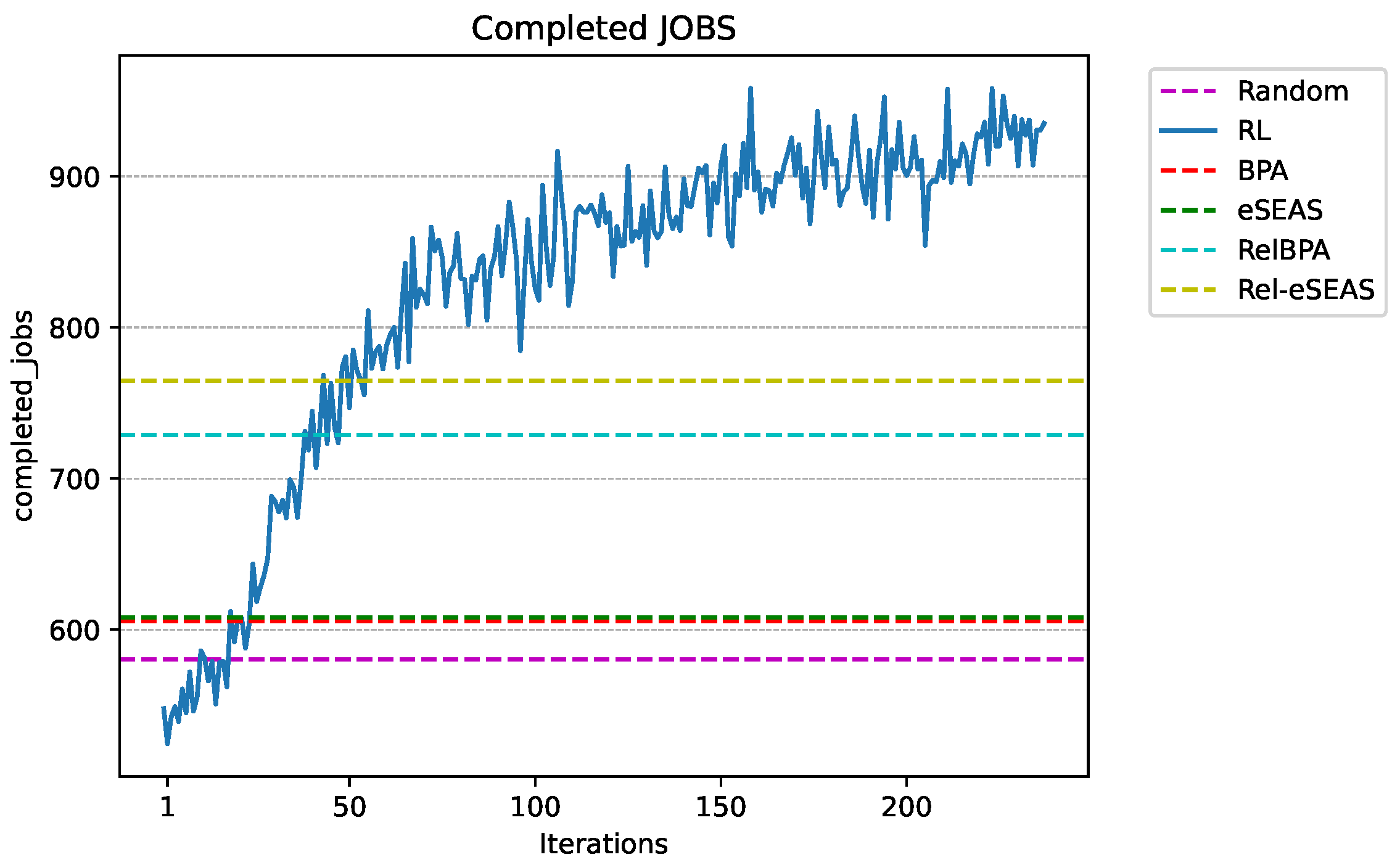
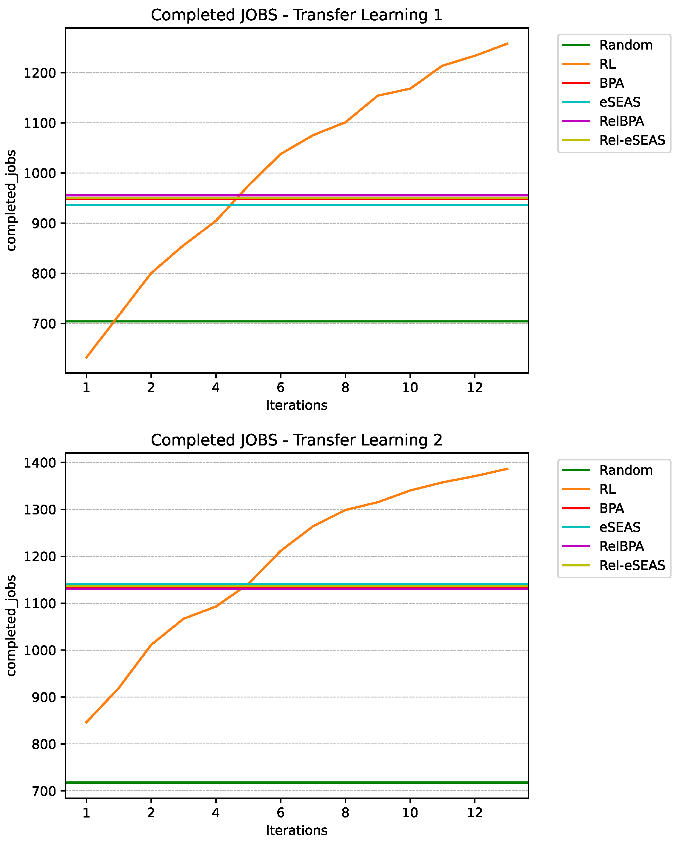
7.5. Reinforcement Learning Agent Results

After the training process described in Section 7.3, we compared the job completion rate with other algorithms using the same simulation environment. The results, as shown in Figure 12, demonstrate that a trained model can quickly adapt to environmental variations and surpass the performance of human-designed job completion heuristics. Notably, around iteration 50, the model in the environment mentioned in Section 7.3 outperforms the best human-designed heuristic regarding job completion, and it continues to improve in this metric in subsequent iterations. One of the challenges in training a reinforcement learning agent for this use case is that the model needs to learn from multiple scenarios to generalize effectively, which is both time-consuming and resource-intensive. However, our objective in this paper is to provide evidence that, despite being trained in different environments, the model can quickly adapt to new ones and excel in the metrics mentioned.

Using the obtained model, we trained new and specific environments using the weights obtained in the first training phase, transferring the learned weights to the new environment. The results show that this new RL agent converges on the job completion rate for each new simulation. Figure 13 details how the agent converges to a solution in each training iteration. The new environments, as said in Section 7.3, were new random waypoint environments, with 1500 JOBS and 25 devices.

7.6. Discussion

We could extract critical results and insights from the experiments for future work. First, the proposed reliability score, which gives a scheduler awareness of node mobility, improves the job completeness metric with regard to human-designed heuristics, not considering such aspect in all run experiments. Moreover, in all experiments, it can be observed that human-crafted policies performed better with random waypoint than with random walk. This result agrees with what the authors in ref. [53] state: random walk is the simplest model, and humans rarely move randomly.

We also showed that RL is viable when the RL agent is adapted to connection and disconnection events. With sufficient training time, RL can devise a solution and even surpass human-crafted policies in terms of job completion rate. Regarding the overfitting problem when the agent needs to be applied in different environments, we suggest training the model with a set of varying environment events data to reduce the probability of overfitting and using the base model as a starting point to specialize one agent version to a specific environment.

8. Conclusions and Future Work

This work presents the EdgeDewSim Extended Simulator, which supports the connection and disconnection of devices into the cluster and its network. With this capability, we were able to experiment with two simple mobility models that tend to simulate a human’s movements and incorporate a new reliability score into two very well-studied algorithms, BPA and E-SEAS [7,22]. The reliability score offers improvements in job completeness and operations executed, which vary depending on the scenario. For future work, it is necessary to extend the mobility models used to generate the connection and disconnection events to reflect real-world human movements more accurately and explore the usage of human-generated movement data to validate the heuristics’ effectiveness. Also, as mentioned in ref. [9], using RL techniques makes it possible to surpass the human-designed heuristics used in this type of environment. However, it is necessary to explore new RL techniques to handle a broader range of dynamic jobs and explore generalization techniques to improve the RL model’s adaptability to diverse environments.

A significant branch of future work involves the practical implementation and testing of the proposed scheduling algorithms in real use-case scenarios. This includes deploying the algorithms in dew computing environments, such as smart city infrastructure or industrial IoT setups, to assess their performance and robustness in real-world conditions. By evaluating the algorithms in diverse applications, we can identify potential challenges, refine them based on real-world feedback, and ensure their readiness for deployment in practical settings. These efforts will bridge the gap between theoretical advancements and practical applicability, paving the way for more reliable and effective device management solutions in dynamic dew computing environments.

References

1. Wang, Y. Definition and categorization of dew computing. Open J. Cloud Comput. (OJCC) 2016, 3, 1–7. [Google Scholar]
2. Ray, P.P. An introduction to dew computing: Definition, concept and implications. IEEE Access 2017, 6, 723–737. [Google Scholar] [CrossRef]
3. Hirsch, M.; Mateos, C.; Zunino, A. Augmenting computing capabilities at the edge by jointly exploiting mobile devices: A survey. Future Gener. Comput. Syst. 2018, 88, 644–662. [Google Scholar] [CrossRef]
4. Khalid, M.N.B. Deep Learning-Based Dew Computing with Novel Offloading Strategy. In Proceedings of the International Conference on Security, Privacy and Anonymity in Computation, Communication and Storage, Nanjing, China, 18–20 December 2020; Springer: Berlin/Heidelberg, Germany, 2020; pp. 444–453. [Google Scholar]
5. Nanakkal, A. A Brief Survey of Future Computing Technologies in Cloud Environment. Ir. Interdiscip. J. Sci. Res. (IIJSR) 2021, 4, 63–70. [Google Scholar] [CrossRef]
6. Hirsch, M.; Rodriguez, J.M.; Zunino, A.; Mateos, C. Battery-aware centralized schedulers for CPU-bound jobs in mobile Grids. Pervasive Mob. Comput. 2016, 29, 73–94. [Google Scholar] [CrossRef]
7. Sanabria, P.; Tapia, T.F.; Neyem, A.; Benedetto, J.I.; Hirsch, M.; Mateos, C.; Zunino, A. New Heuristics for Scheduling and Distributing Jobs under Hybrid Dew Computing Environments. Wirel. Commun. Mob. Comput. 2021, 2021, 8899660. [Google Scholar] [CrossRef]
8. Samal, P.; Mishra, P. Analysis of variants in Round Robin Algorithms for load balancing in Cloud Computing. Int. J. Comput. Sci. Inf. Technol. 2013, 4, 416–419. [Google Scholar]
9. Sanabria, P.; Tapia, T.F.; Toro Icarte, R.; Neyem, A. Solving Task Scheduling Problems in Dew Computing via Deep Reinforcement Learning. Appl. Sci. 2022, 12, 7137. [Google Scholar] [CrossRef]
10. Sutton, R.S.; Barto, A.G. Reinforcement Learning: An Introduction; MIT Press: Cambridge, MA, USA, 2018. [Google Scholar]
11. Akkaya, I.; Andrychowicz, M.; Chociej, M.; Litwin, M.; McGrew, B.; Petron, A.; Paino, A.; Plappert, M.; Powell, G.; Ribas, R.; et al. Solving rubik’s cube with a robot hand. arXiv 2019, arXiv:1910.07113. [Google Scholar]
12. Li, J.; Monroe, W.; Ritter, A.; Galley, M.; Gao, J.; Jurafsky, D. Deep reinforcement learning for dialogue generation. arXiv 2016, arXiv:1606.01541. [Google Scholar]
13. Popova, M.; Isayev, O.; Tropsha, A. Deep reinforcement learning for de novo drug design. Sci. Adv. 2018, 4, eaap7885. [Google Scholar] [CrossRef] [PubMed]
14. Mao, Y.; You, C.; Zhang, J.; Huang, K.; Letaief, K.B. A survey on mobile edge computing: The communication perspective. IEEE Commun. Surv. Tutorials 2017, 19, 2322–2358. [Google Scholar] [CrossRef]
15. Khan, W.Z.; Ahmed, E.; Hakak, S.; Yaqoob, I.; Ahmed, A. Edge computing: A survey. Future Gener. Comput. Syst. 2019, 97, 219–235. [Google Scholar] [CrossRef]
16. Drolia, U.; Martins, R.; Tan, J.; Chheda, A.; Sanghavi, M.; Gandhi, R.; Narasimhan, P. The case for mobile edge-clouds. In Proceedings of the 2013 IEEE 10th International Conference on Ubiquitous Intelligence and Computing and 2013 IEEE 10th International Conference on Autonomic and Trusted Computing, Vietri sul Mare, Italy, 18–21 December 2013; IEEE: Vietri sul Mare, Italy, 2013; pp. 209–215. [Google Scholar]
17. Benedetto, J.I.; González, L.A.; Sanabria, P.; Neyem, A.; Navón, J. Towards a practical framework for code offloading in the Internet of Things. Future Gener. Comput. Syst. 2019, 92, 424–437. [Google Scholar] [CrossRef]
18. Shi, W.; Cao, J.; Zhang, Q.; Li, Y.; Xu, L. Edge computing: Vision and challenges. IEEE Internet Things J. 2016, 3, 637–646. [Google Scholar] [CrossRef]
19. Yu, W.; Liang, F.; He, X.; Hatcher, W.G.; Lu, C.; Lin, J.; Yang, X. A survey on the edge computing for the Internet of Things. IEEE Access 2017, 6, 6900–6919. [Google Scholar] [CrossRef]
20. Olaniyan, R.; Fadahunsi, O.; Maheswaran, M.; Zhani, M.F. Opportunistic edge computing: Concepts, opportunities and research challenges. Future Gener. Comput. Syst. 2018, 89, 633–645. [Google Scholar] [CrossRef]
21. Aslam, S.; Michaelides, M.P.; Herodotou, H. Internet of ships: A survey on architectures, emerging applications, and challenges. IEEE Internet Things J. 2020, 7, 9714–9727. [Google Scholar] [CrossRef]
22. Hirsch, M.; Rodriguez, J.M.; Mateos, C.; Alejandro, Z. A Two-Phase Energy-Aware Scheduling Approach for CPU-Intensive Jobs in Mobile Grids. J. Grid Comput. 2017, 15, 55–80. [Google Scholar] [CrossRef]
23. Hirsch, M.; Mateos, C.; Rodriguez, J.M.; Zunino, A.; Garí, Y.; Monge, D.A. A performance comparison of data-aware heuristics for scheduling jobs in mobile grids. In Proceedings of the 2017 XLIII Latin American Computer Conference (CLEI), Córdoba, Argentina, 4–8 September 2017; IEEE: Córdoba, Argentina, 2017; pp. 1–8. [Google Scholar]
24. Chen, X.; Pu, L.; Gao, L.; Wu, W.; Wu, D. Exploiting Massive D2D Collaboration for Energy-Efficient Mobile Edge Computing. IEEE Wirel. Commun. 2017, 24, 64–71. [Google Scholar] [CrossRef]
25. Mtibaa, A.; Fahim, A.; Harras, K.A.; Ammar, M.H. Towards resource sharing in mobile device clouds. ACM SIGCOMM Comput. Commun. Rev. 2013, 43, 51–56. [Google Scholar] [CrossRef]
26. Li, B.; Pei, Y.; Wu, H.; Shen, B. Heuristics to allocate high-performance cloudlets for computation offloading in mobile ad hoc clouds. J. Supercomput. 2015, 71, 3009–3036. [Google Scholar] [CrossRef]
27. Chunlin, L.; Layuan, L. Exploiting composition of mobile devices for maximizing user QoS under energy constraints in mobile grid. Inf. Sci. 2014, 279, 654–670. [Google Scholar] [CrossRef]
28. Birje, M.N.; Manvi, S.S.; Das, S.K. Reliable resources brokering scheme in wireless grids based on non-cooperative bargaining game. J. Netw. Comput. Appl. 2014, 39, 266–279. [Google Scholar] [CrossRef]
29. Loke, S.W.; Napier, K.; Alali, A.; Fernando, N.; Rahayu, W. Mobile Computations with Surrounding Devices. ACM Trans. Embed. Comput. Syst. 2015, 14, 1–25. [Google Scholar] [CrossRef]
30. Shah, S.C. Energy efficient and robust allocation of interdependent tasks on mobile ad hoc computational grid. Concurr. Comput. Pract. Exp. 2015, 27, 1226–1254. [Google Scholar] [CrossRef]
31. Orhean, A.I.; Pop, F.; Raicu, I. New scheduling approach using reinforcement learning for heterogeneous distributed systems. J. Parallel Distrib. Comput. 2018, 117, 292–302. [Google Scholar] [CrossRef]
32. Kaur, P. DRLCOA: Deep Reinforcement Learning Computation Offloading Algorithm in Mobile Cloud Computing. SSRN Electron. J. 2019, 12, 238–246. [Google Scholar] [CrossRef]
33. Cheng, M.; Li, J.; Nazarian, S. DRL-cloud: Deep reinforcement learning-based resource provisioning and task scheduling for cloud service providers. In Proceedings of the 2018 23rd Asia and South Pacific Design Automation Conference (ASP-DAC), Jeju, Republic of Korea, 22–25 January 2018; IEEE: Jeju, Republic of Korea, 2018; pp. 129–134. [Google Scholar] [CrossRef]
34. Huang, L.; Bi, S.; Zhang, Y.J.A. Deep Reinforcement Learning for Online Computation Offloading in Wireless Powered Mobile-Edge Computing Networks. IEEE Trans. Mob. Comput. 2020, 19, 2581–2593. [Google Scholar] [CrossRef]
35. Ha, S.; Choi, E.; Ko, D.; Kang, S.; Lee, S. Efficient Resource Augmentation of Resource Constrained UAVs Through EdgeCPS. In Proceedings of the 38th ACM/SIGAPP Symposium on Applied Computing, Tallinn, Estonia, 27–31 March 2023; pp. 679–682. [Google Scholar]
36. Ren, J.; Xu, S. DDPG Based Computation Offloading and Resource Allocation for MEC Systems with Energy Harvesting. In Proceedings of the 2021 IEEE 93rd Vehicular Technology Conference (VTC2021-Spring), Virtual, 25 April–19 May 2021; IEEE: Helsinki, Finland, 2021; pp. 1–5. [Google Scholar]
37. Zhao, R.; Wang, X.; Xia, J.; Fan, L. Deep reinforcement learning based mobile edge computing for intelligent Internet of Things. Phys. Commun. 2020, 43, 101184. [Google Scholar] [CrossRef]
38. Tefera, G.; She, K.; Shelke, M.; Ahmed, A. Decentralized adaptive resource-aware computation offloading & caching for multi-access edge computing networks. Sustain. Comput. Inform. Syst. 2021, 30, 100555. [Google Scholar] [CrossRef]
39. Baek, J.; Kaddoum, G. Heterogeneous Task Offloading and Resource Allocations via Deep Recurrent Reinforcement Learning in Partial Observable Multi-Fog Networks. IEEE Internet Things J. 2020, 8, 1041–1056. [Google Scholar] [CrossRef]
40. Lu, H.; Gu, C.; Luo, F.; Ding, W.; Liu, X. Optimization of lightweight task offloading strategy for mobile edge computing based on deep reinforcement learning. Future Gener. Comput. Syst. 2020, 102, 847–861. [Google Scholar] [CrossRef]
41. Li, J.; Gao, H.; Lv, T.; Lu, Y. Deep reinforcement learning based computation offloading and resource allocation for MEC. In Proceedings of the 2018 IEEE Wireless Communications and Networking Conference (WCNC), Barcelona, Spain, 15–18 April 2018; IEEE: Barcelona, Spain, 2018; pp. 1–6. [Google Scholar] [CrossRef]
42. Alfakih, T.; Hassan, M.M.; Gumaei, A.; Savaglio, C.; Fortino, G. Task Offloading and Resource Allocation for Mobile Edge Computing by Deep Reinforcement Learning Based on SARSA. IEEE Access 2020, 8, 54074–54084. [Google Scholar] [CrossRef]
43. Zhao, L.; Li, H.; Zhang, E.; Hawbani, A.; Lin, M.; Wan, S.; Guizani, M. Intelligent Caching for Vehicular Dew Computing in Poor Network Connectivity Environments. ACM Trans. Embed. Comput. Syst. 2024, 23, 1–24. [Google Scholar] [CrossRef]
44. Khatua, S.; Manerba, D.; Maity, S.; De, D. Dew Computing-Based Sustainable Internet of Vehicular Things. In Dew Computing: The Sustainable IoT Perspectives; Springer: Berlin/Heidelberg, Germany, 2023; pp. 181–205. [Google Scholar]
45. Pal, M.N.; Sengupta, D.; Tran, T.A.; De, D. Machine Learning-Based Sustainable Dew Computing: Classical to Quantum. In Dew Computing: The Sustainable IoT Perspectives; Springer: Berlin/Heidelberg, Germany, 2023; pp. 149–177. [Google Scholar]
46. Chakraborty, S.; De, D.; Mazumdar, K. DoME: Dew computing based microservice execution in mobile edge using Q-learning. Appl. Intell. 2023, 53, 10917–10936. [Google Scholar] [CrossRef]
47. Cobbe, K.; Klimov, O.; Hesse, C.; Kim, T.; Schulman, J. Quantifying generalization in reinforcement learning. In Proceedings of the 36th International Conference on Machine Learning (ICML), Long Beach, CA, USA, 9–15 June 2019; pp. 1282–1289. [Google Scholar]
48. Cobbe, K.; Hesse, C.; Hilton, J.; Schulman, J. Leveraging procedural generation to benchmark reinforcement learning. In Proceedings of the 37th International Conference on Machine Learning (ICML), Virtual Event, 13–18 July 2020; pp. 2048–2056. [Google Scholar]
49. Hirsch, M.; Mateos, C.; Rodriguez, J.M.; Zunino, A. DewSim: A trace-driven toolkit for simulating mobile device clusters in Dew computing environments. Softw. Pract. Exp. 2020, 50, 688–718. [Google Scholar] [CrossRef]
50. Manweiler, J.; Santhapuri, N.; Choudhury, R.R.; Nelakuditi, S. Predicting length of stay at wifi hotspots. In Proceedings of the 2013 IEEE INFOCOM, Turin, Italy, 14–19 April 2013; pp. 3102–3110. [Google Scholar]
51. Blanford, J.I.; Huang, Z.; Savelyev, A.; MacEachren, A.M. Geo-located tweets. Enhancing mobility maps and capturing cross-border movement. PLoS ONE 2015, 10, e0129202. [Google Scholar] [CrossRef]
52. Barbosa, H.; Barthelemy, M.; Ghoshal, G.; James, C.R.; Lenormand, M.; Louail, T.; Menezes, R.; Ramasco, J.J.; Simini, F.; Tomasini, M. Human mobility: Models and applications. Phys. Rep. 2018, 734, 1–74. [Google Scholar] [CrossRef]
53. Solmaz, G.; Turgut, D. A Survey of Human Mobility Models. IEEE Access 2019, 7, 125711–125731. [Google Scholar] [CrossRef]
54. Falaki, H.; Mahajan, R.; Kandula, S.; Lymberopoulos, D.; Govindan, R.; Estrin, D. Diversity in Smartphone Usage. In Proceedings of the 8th International Conference on Mobile Systems, Applications, and Services (MobiSys’10), New York, NY, USA, 15–18 June 2010; pp. 179–194. [Google Scholar] [CrossRef]
55. Keramat Jahromi, K.; Zignani, M.; Gaito, S.; Rossi, G.P. Simulating human mobility patterns in urban areas. Simul. Model. Pract. Theory 2016, 62, 137–156. [Google Scholar] [CrossRef]
56. Henderson, T.; Kotz, D.; Abyzov, I. The changing usage of a mature campus-wide wireless network. Comput. Netw. 2008, 52, 2690–2712. [Google Scholar] [CrossRef]
57. Gorawski, M.; Grochla, K. Review of mobility models for performance evaluation of wireless networks. In Man-Machine Interactions 3; Springer: Berlin/Heidelberg, Germany, 2014; pp. 567–577. [Google Scholar]
58. Panisson, A. Pymobility v0.1—Python Implementation of Mobility Models. 2015. Available online: https://zenodo.org/records/9873 (accessed on 27 November 2023).
59. Zhao, K.; Tarkoma, S.; Liu, S.; Vo, H. Urban human mobility data mining: An overview. In Proceedings of the 2016 IEEE International Conference on Big Data (Big Data), Washington, DC, USA, 5–8 December 2016; pp. 1911–1920. [Google Scholar]
60. Brockman, G.; Cheung, V.; Pettersson, L.; Schneider, J.; Schulman, J.; Tang, J.; Zaremba, W. Openai gym. arXiv 2016, arXiv:1606.01540. [Google Scholar]
61. Zhang, A.; Ballas, N.; Pineau, J. A dissection of overfitting and generalization in continuous reinforcement learning. arXiv 2018, arXiv:1806.07937. [Google Scholar]
62. Zhang, C.; Vinyals, O.; Munos, R.; Bengio, S. A study on overfitting in deep reinforcement learning. arXiv 2018, arXiv:1804.06893. [Google Scholar]
Figure 1. Example of SCE architecture: In this example, six devices are connected to the local network. The devices include two smartphones, two Raspberry Pis, two laptops, and one scheduler inside the network. Outside of the network are two smartphones.
Applsci 14 03206 g001
Figure 2. Training loop of the EdgeDewSim Extended Simulator environment.
Applsci 14 03206 g002
Figure 3. Sequence diagram of one job scheduling with an external environment.
Applsci 14 03206 g003
Figure 4. Average job completion for each simulation using random walk to generate connection events and the 1500 jobs set.
Applsci 14 03206 g004
Figure 5. Average job completion for each simulation using random waypoint to generate connection events and the 1500 jobs set.
Applsci 14 03206 g005
Figure 6. Average job completion for each simulation using random walk to generate connection events and the full set of jobs.
Applsci 14 03206 g006
Figure 7. Average job completion for each simulation using random waypoint to generate connection events and the full set of jobs.
Applsci 14 03206 g007
Figure 8. Average performance in GIPS for each simulation using random walk to generate connection events and the 1500 jobs set.
Applsci 14 03206 g008
Figure 9. Average performance in GIPS for each simulation using random walk to generate connection events and the full set of jobs.
Applsci 14 03206 g009
Figure 10. Average performance in GIPS for each simulation using random waypoint to generate connection events and the 1500 jobs set.
Applsci 14 03206 g010
Figure 11. Average performance in GIPS for each simulation using random waypoint to generate connection events and the full set of jobs.
Applsci 14 03206 g011
Figure 12. RL convergence for job completion for each simulation using random walk compared to other algorithms in the 1500 jobs set.
Applsci 14 03206 g012
Figure 13. RL Convergence for job completion for each simulation using transfer learning in a random waypoint environment compared to other algorithms in the 1500 jobs set.
Applsci 14 03206 g013