Abstract
Knowledge distillation based on the features from the penultimate layer allows the student (lightweight model) to efficiently mimic the internal feature outputs of the teacher (high-capacity model). However, the training data may not conform to the ground-truth distribution of images in terms of classes and features. We propose two knowledge distillation algorithms to solve the above problem from the directions of fitting the ground-truth distribution of classes and fitting the ground-truth distribution of features, respectively. The former uses teacher labels to supervise student classification output instead of dataset labels, while the latter designs feature temperature parameters to correct teachers’ abnormal feature distribution output. We conducted knowledge distillation experiments on the ImageNet-2012 and Cifar-100 datasets using seven sets of homogeneous models and six sets of heterogeneous models. The experimental results show that our proposed algorithms improve the performance of penultimate layer feature knowledge distillation and outperform other existing knowledge distillation methods in terms of classification performance and generalization ability.
1. Introduction
Deep learning neural networks play a significant role in computer vision applications such as image classification [1,2,3], object detection [4,5,6], and semantic segmentation [7,8,9]. However, since computational resources are often limited in mobile scenarios, high-accuracy models with high computational loads are unsuitable for these applications. Furthermore, lightweight models may not meet the performance and accuracy requirements of practical applications. To address this issue, Hinton et al. [10] introduced knowledge distillation (KD), which involves supervising a student network’s training by extracting logits output from the teacher network. Throughout the development of knowledge distillation, there has been considerable focus on feature distillation [11,12]. However, most feature distillation is based on middle-layer features in neural networks, with little emphasis on utilizing the features from the penultimate layer.
Penultimate layer feature knowledge distillation transfers knowledge by extracting the penultimate layer feature representation of the teacher model and minimizing the distance between it and the student’s penultimate layer features. In this way, students learn the abstract features contained in the teacher’s model. Logit distillation aims to make students learn the ability to map and categorize feature maps. In comparison, the penultimate layer of feature distillation focuses more on learning the feature map representation ability. In contrast to knowledge distillation using intermediate layer features, the penultimate layer features are obtained through multi-layer transformations of neural networks, which usually have a higher level of abstraction and semantic information. Recently, Wang et al. [13] used the penultimate layer outputs as distillation knowledge, combining locality-sensitive hashing (LSH) loss with mean square loss, achieving the ability to fit both feature directions and magnitudes effectively.
LSH [13] is an effective algorithm for knowledge distillation that can match features in the penultimate layer of teacher and student. However, some important considerations must be addressed.
Firstly, due to the visual similarity between images, one-hot labels cannot accurately describe the ground-truth distribution based on classes [14]. We use an example of a binary classification task of tigers and lions. The training data for tigers in the dataset are labelled as (1,0), indicating that these training data are a tigers. However, the label for the ground-truth distribution of images based on classes is (0.7,0.3). The reason for this difference is that the category’s ground-truth distribution consists of feature correlations. Because there is a partial visual similarity between lions and tigers, a small number of category label values are assigned to the lion category. In the paper [14], the difference between the dataset labels and the image’s ground-truth distribution of classes was considered as label noise. Incorrect labels could potentially have a negative impact on training [15].
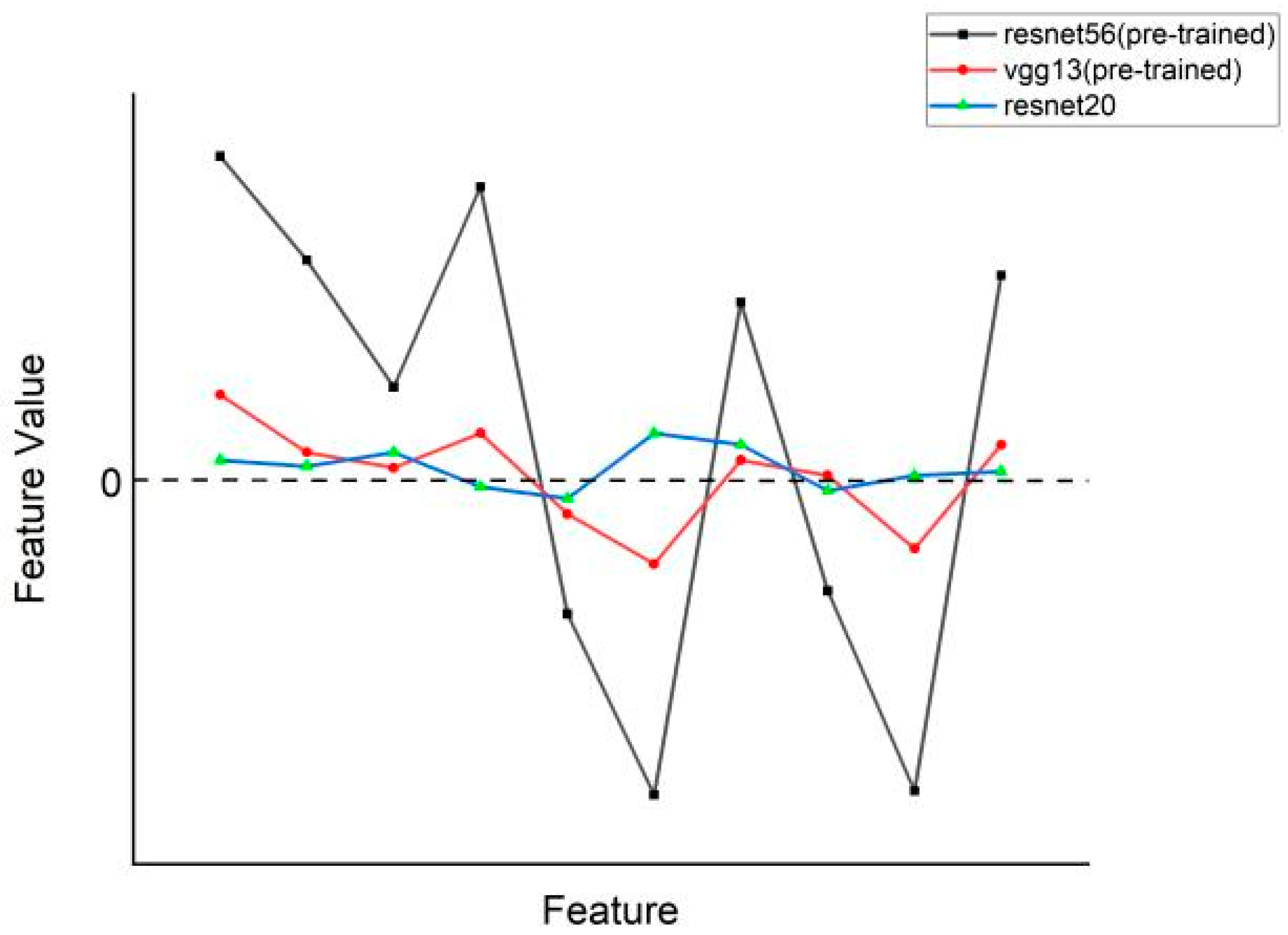
Secondly, the penultimate layer feature outputs of some pre-trained teacher models (such as vgg13, resnet32×4, etc.) are generally lower. These were found in the penultimate layer feature distillation experiments. As shown in Figure 1, we extracted some of the feature values from the penultimate layer output of the model from the pre-trained resnet56, the pre-trained vgg13, and the untrained resnet20. The distribution of feature values in the figure shows that the pre-trained resnet56 discriminates feature values between important and non-important features. Because resnet20 is not trained, it is difficult to distinguish between important and non-important features, so it assigns lower eigenvalues to each feature. The pre-trained vgg13 can distinguish between important and non-important features (important features have higher feature values than non-important features), but the overall feature differentiation is small. Because of the lack of distinctiveness in penultimate layer feature outputs, it cannot accurately represent the ground-truth feature distribution of images.
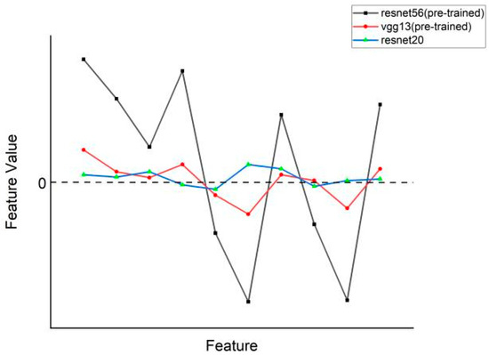
Figure 1.
Distribution of features in the penultimate layer of resent56 (pre-trained), vgg13 (pre-trained), and resnet20.
Knowledge distillation is a compression algorithm in which students learn the ground-truth distribution of images in real task scenarios by fitting the teacher’s output. The reason why this type of learning works is that the teacher can learn about the task in advance and output data that more closely matches the ground-truth distribution to provide knowledge to the students. These learning data do not necessarily conform to the true distribution for the reasons mentioned above. This discrepancy makes it difficult for students to learn more effectively, thus reducing the performance of knowledge distillation. To tackle these challenges, the main contributions can be summarized as follows:
- We propose a knowledge distillation algorithm based on fitting the ground-truth distributions of classes (locality-sensitive hashing—teacher label, LSH-TL), which uses the teacher’s classification labels instead of one-hot labels to reduce the negative impact on distillation caused by label noise between the ground-truth distribution of classes and the dataset one-hot label. Experimental results on the CIFAR-100 and ImageNet-2012 image classification datasets demonstrate that this method enhances feature distillation at the penultimate layer;
- To address situations where the distribution of feature outputs at the penultimate layer in some models is lower than the ground-truth feature distribution, we propose a knowledge distillation algorithm based on fitting the ground-truth distributions of features (locality-sensitive hashing—temperature, LSH-T), which enhances feature mimicry by introducing the feature temperature. This improvement significantly alleviates the issue of overly smooth feature outputs in teacher models. Extensive experiments involving the distillation of various model groups demonstrate that this approach outperforms other distillation methods.
2. Related Work
The earliest source of knowledge in knowledge distillation is response-based. Hinton et al. [10] involves applying Softmax to the classification outputs of the student and teacher models to generate soft logits. Using the soft logits to calculate the KL-divergence loss for knowledge transfer. Zhao et al. [16] introduced a decoupling and analysis approach to KD. It separates logits into target and non-target classes, assigning greater weight to the more informative non-target classes. This method can make more effective use of the logits information of the teacher and further improve the performance of knowledge distillation based on response.
Non-response-based knowledge distillation focuses on relationships between samples or feature layers. Romero et al. [11] extended the knowledge distillation proposed by Hinton and designed FitNets. It begins by using intermediate layer features of the teacher model as the knowledge to be distilled. Zagoruyko et al. [17] proposed the improvement of network performance through attention transfer (AT). Heo et al. [18] argued that distillation supervision should not only be based on neuron activation values but should also consider the neuron activation boundary (AB). Tung et al. [19] found that similar semantic input will produce similar activation in a trained network and proposed similarity-preserving (SP) knowledge distillation. Yim et al. [20] utilized the inner product between feature layers to obtain the FSP matrix for knowledge distillation. Kim et al. [21] introduced factors as an interpretable form of intermediate layer features to implement factor transfer (FT). Tian et al. [12] proposed contrastive representation distillation (CRD) to bring the student closer to the teacher on outputs of the same class while pushing them further apart on outputs of different classes. Xu et al. [22] proposed self-supervised knowledge distillation (SSKD) which designed a self-supervised module to identify hidden knowledge. Wang et al. [13] combined the model’s penultimate layer outputs with a locality-sensitive hashing algorithm for knowledge distillation, achieving excellent results on the majority of distillation model groups.
The distillation knowledge used in KD [10] comes from the output of the model classification layer after Softmax. FitNet [11], AT [17], and AB [18] use distillation knowledge from intermediate layers of the model. We observed that there has been limited research focused on the model’s penultimate layer features. Our work is related to the LSH [13] algorithm, which allows students to fit the feature output of the teacher’s penultimate layer by designing a knowledge distillation algorithm based on location-sensitive hashing. However, it did not further explore the potential feature learning ability of the model’s penultimate layer. We improve distillation performance by mapping image classification and feature output distributions to ground-truth distribution of images.
3. Method
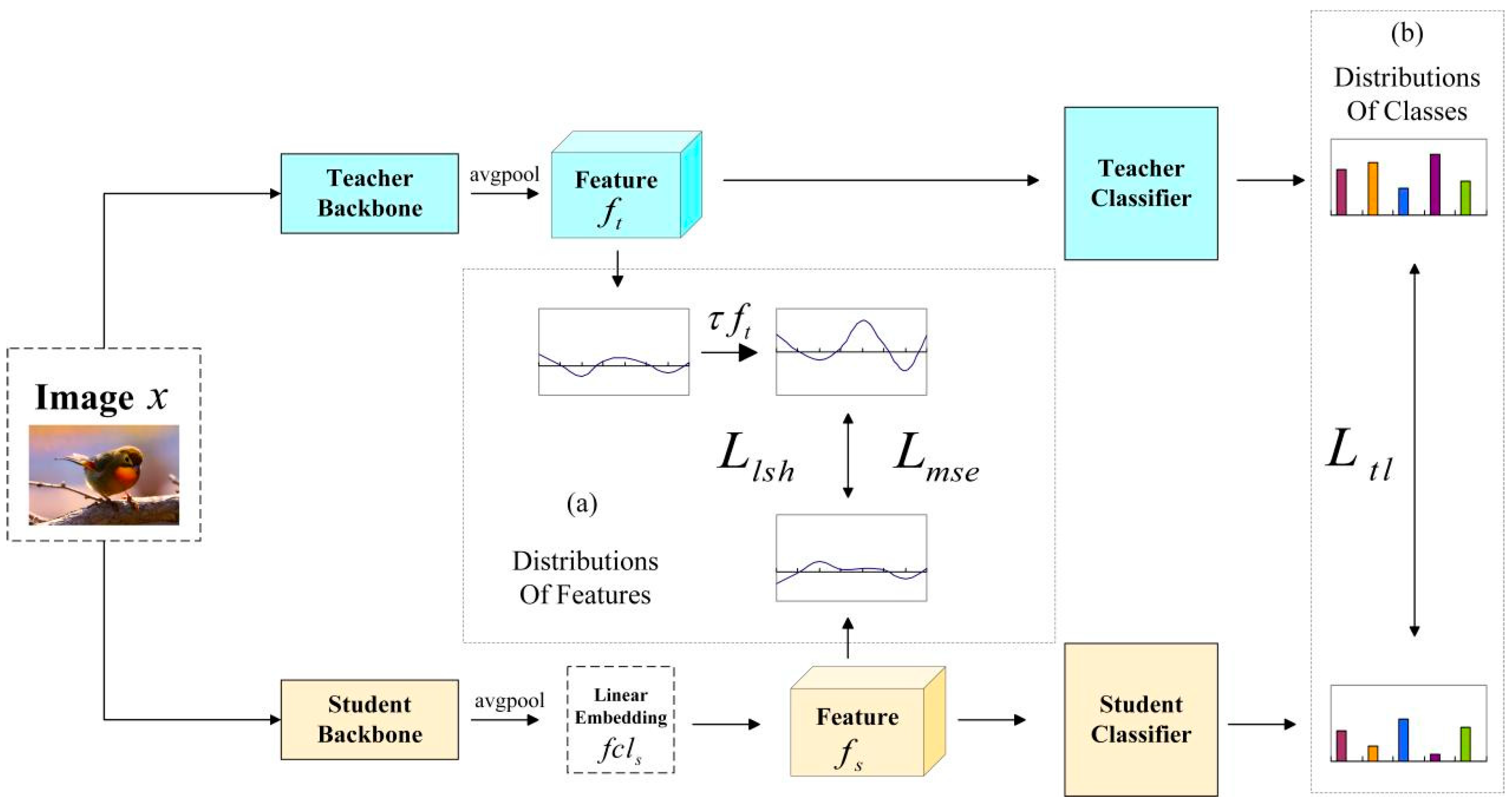
The overall framework is shown in Figure 2. For a given image data x, all images are cropped to the same size via image preprocessing operations and fed into the teacher backbone network and student backbone network respectively. Teachers usually refer to complex networks that have been pre-trained and have a certain feature recognition capability. Students refer to untrained, smaller, as well as lighter networks relative to teachers. In the teacher and student backbone networks, the data undergo a layer-by-layer feature extraction that captures the main information in the data and outputs a data matrix in each layer. The data are processed through the backbone network and changed into a one-dimensional matrix through the average pool (avgpool) layer, which outputs the features of the penultimate layer. The teacher backbone network can extract features which are the penultimate layer feature outputs of the teacher network. The student backbone network also extracts the penultimate features and fits for knowledge distillation.
When conducting knowledge distillation using the model’s penultimate layer outputs, especially in the case of heterogeneous model distillation, we encounter the issue of mismatched dimensions between the student’s feature dimension and the teacher’s feature dimension . Therefore, a linear embedding layer is added to complete the dimension matching between teacher and student:
and are the weight and bias parameters of the embedded layer which are updated via loss backward in training. After the student backbone network output enters , it will output the student feature with dimension .
The loss function used is as follows. is defined as the mean squared error loss:
where represents the number of samples. denotes the feature dimension. represents input image data. and , respectively, represent the penultimate layer feature outputs of the teacher model and the student model for the image in the dataset.
is locality-sensitive hashing knowledge distillation:
builds upon by introducing locality-sensitive hashing loss (). The cross-entropy loss is used as the classification loss. and are balancing weights. is locality-sensitive hashing loss:
where represents the teacher’s hash and represents the student’s hash:
is the weight sampled from the Gaussian distribution and is the bias. Equation (5) generates hashes for each feature.
LSH extracts the correctly classified teacher features through the function. The calculation of the hash value can be implemented via the linear layer in the neural network. The purpose is to match the hash of the student features with the hash of the teacher’s correct classification features.
When the teacher and the student have completed their respective feature extraction, the penultimate layers of features are mapped into a classifier equal in size to the number of categories in the dataset. The distribution of image categories judged by the network is the output in the classifier. The class with the largest category value obtained is the class to which the network has judged this image to belong.
As shown in Figure 2. Based on LSH [13], we designed two different knowledge distillation algorithms based on ground-truth distribution fitting of images. The two algorithms are LSH-T and LSH-TL. LSH-T fits the ground-truth distribution of features, while LSH-TL fits the ground-truth distribution of classes. Figure 2a illustrates the method for fitting the ground-truth distribution of features (LSH-T). We address the overly smooth feature distribution of the penultimate layer by introducing a feature temperature to correct the penultimate layer feature output of the teacher. After the feature temperature treatment, the penultimate layer feature output of the teacher obtains greater discriminability of features and the feature distribution becomes sharper. In the process of distilling the penultimate layer of feature knowledge with and , the teacher can provide students with more significant feature relevance information; Figure 2b shows the fitting method of the ground-truth distribution of classes (LSH-TL). The original LSH used dataset labels to supervise student classifier outputs. We believe that there is a discrepancy between the dataset labels and the ground-truth distribution of image classes. Because the teacher has been pre-trained in the relevant task scenarios, the teacher can output category distributions that are similar to the ground-truth distribution. So, we extract the teacher classifier output to supervise the output of the student classifier without using the dataset labels. Such supervision is more in line with the need for the penultimate layer of feature knowledge distillation for fitting the ground-truth distribution.

Figure 2.
The overall framework: (a) the ground-truth distribution fitting method of features (LSH-T); (b) the ground-truth distribution fitting method of classes (LSH-TL), Each color represents a distinct class.
Figure 2.
The overall framework: (a) the ground-truth distribution fitting method of features (LSH-T); (b) the ground-truth distribution fitting method of classes (LSH-TL), Each color represents a distinct class.
3.1. Fitting The Ground-Truth Distributions of Classes (LSH-TL)
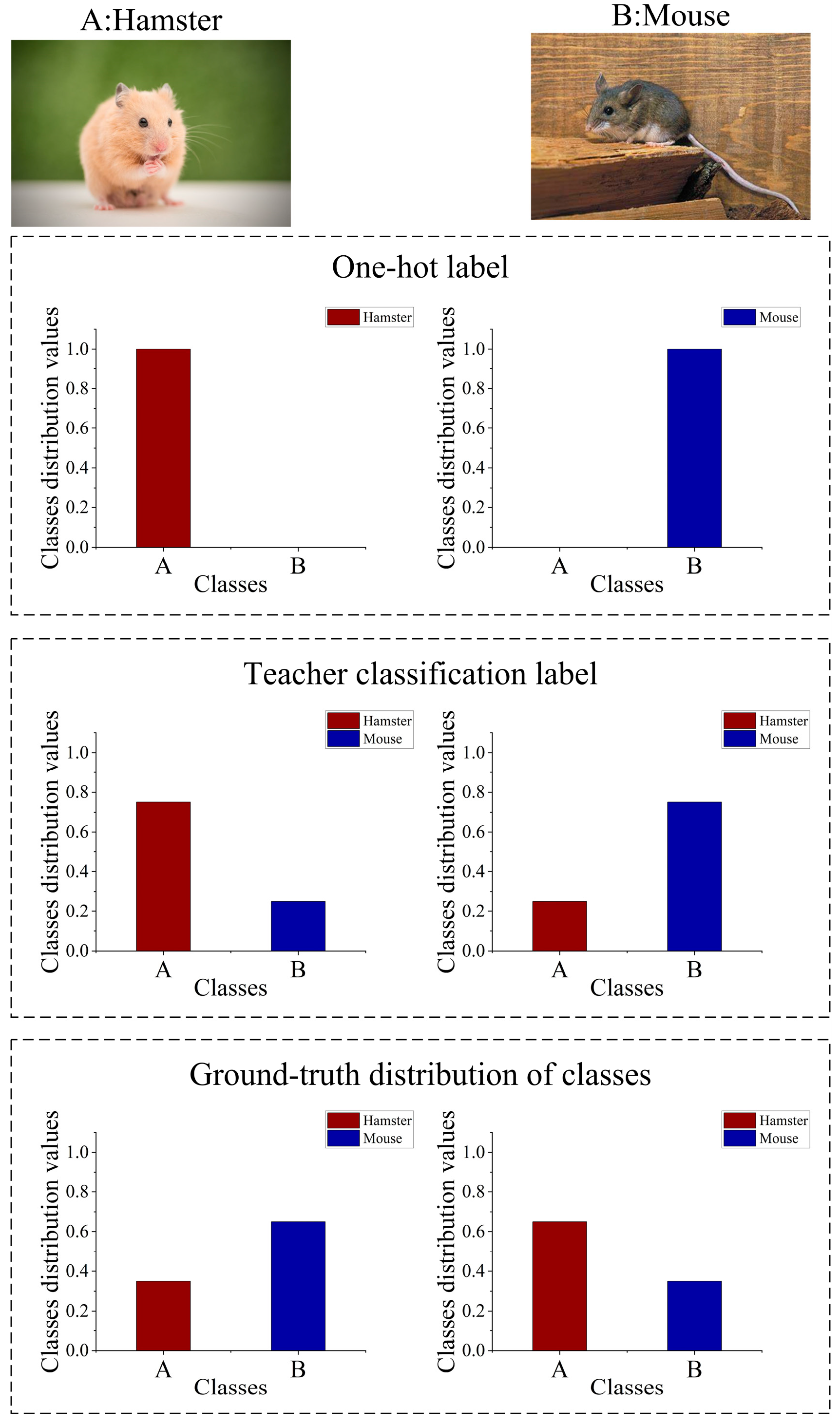
Due to the visually similar features between images, one-hot labels cannot accurately describe the ground-truth distribution of classes determined by features, as shown in Figure 3. The model assigns values to classification categories based on the features. Because hamsters and mice share similarities, the one-hot labels only represent single values for categories, which cannot reflect the ground-truth distribution of classes. Teacher classification label output by the pre-training teacher is closer to the ground-truth distribution of classes.
To solve this problem, we replaced the one-hot label with the teacher classification label. Because the classification layer is below the penultimate layer, the student autonomously learns the teacher’s classification output while mimicking the teacher’s penultimate layer features. Therefore, learning the teacher classification label allows the student to focus more on mimicking the feature.
We utilize the to supervise the student’s classification output with the teacher classification label. is defined as follows:
where represents the score logits, I is the category index, x is the data sample, t and s denote teacher and student, C is the total number of classes, and Dx indicates the dataset.
Replacing with in LSH, is the balancing weight of . The loss function of LSH-TL is as follows:

Figure 3.
The differences among the one-hot label, teacher classification label, and ground-truth distribution of classes.
Figure 3.
The differences among the one-hot label, teacher classification label, and ground-truth distribution of classes.
3.2. Fitting the Ground-Truth Distributions of Features (LSH-T)
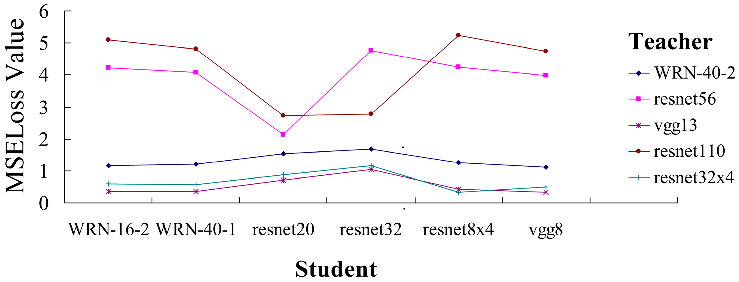
When the distillation training stage is at epoch 0, the penultimate layer feature losses between some distillation teacher–student groups are quite low, which is almost equal to the feature loss value of some distillation teacher–student groups that have completed the training. We show some examples in Figure 4. The penultimate layer feature losses between the pre-trained teachers (vgg13, resnet32×4, and WRN-40-2) and untrained students are significantly lower. On the contrary, the penultimate layer feature losses are relatively normal when resnet110 and resnet56 are used as pre-training teachers. We believe that overly low feature loss is harmful to feature distillation in the penultimate layer, which limits the potential of feature mimicking.
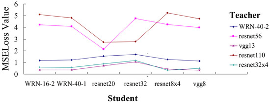
Figure 4.
The MSE loss values (y-axis) between teachers (different colored lines) and students (x-axis) when the distillation training stage is at epoch 0 epoch.
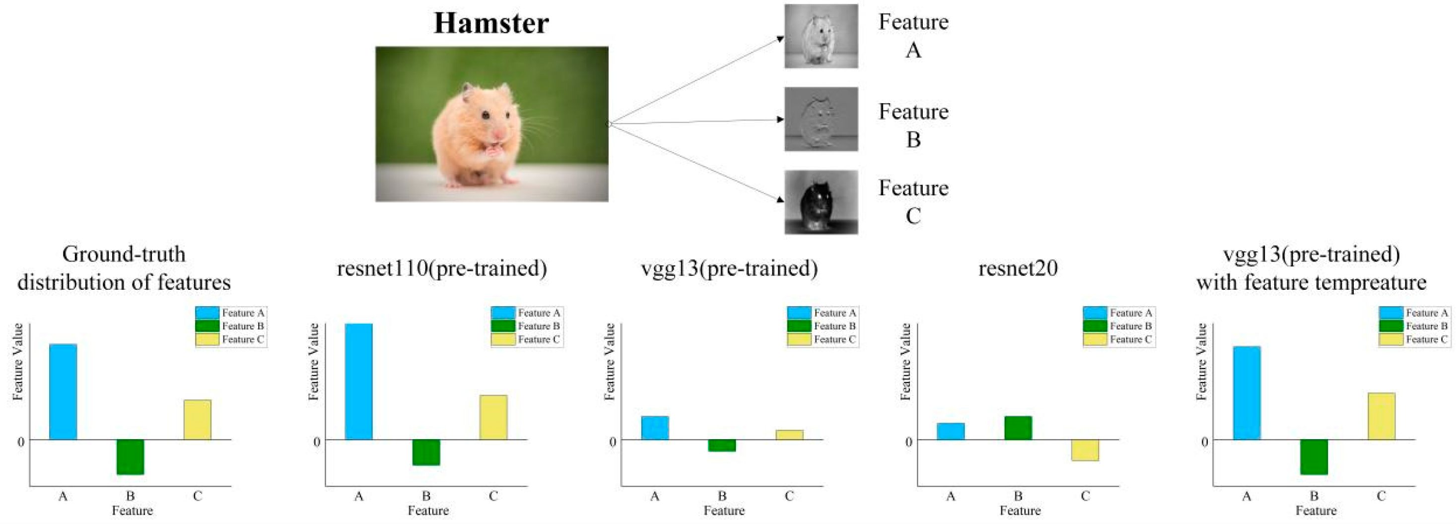
This phenomenon can be explained using Figure 5. In normal circumstances, features that are more relevant to the image tend to receive higher feature values. In the real feature distribution of images, feature A is the most important feature and feature B is the least important feature. The pre-trained resnet110 includes feature recognition ability and can assign appropriate feature values to each feature. Untrained resnet20’s feature recognition ability is relatively low, and it is impossible to determine which features are important. It assigns relatively average and lower feature values to all features. Therefore, when resnet110 and resnet56 serve as teachers in Figure 5 they maintain a relatively high feature loss when facing all students. In the penultimate layer of feature distillation, the student gradually reduces feature loss by learning the feature recognition ability from the teacher.
In abnormal circumstances, the pre-trained vgg13 assigns low feature values to all features, even though the feature value of the most important feature (A) remains the highest compared to other features (B, C). However, the feature loss between teacher and student remains low. This makes feature mimicking more difficult during the distillation process.
In order to solve the above problems, we introduce the feature temperature () as a corrective factor to improve the teacher’s feature output:
As shown in Figure 5. By introducing the feature temperature parameter, we can enhance the distinguishability between important features and other features. Make the overall feature distribution of the teacher closer to the ground-truth distribution of features and release the potential of feature mimicking. The loss function of LSH-T is as follows:
By introducing the feature temperature parameter, we widen the gap between the feature values of important and non-important features. However, the relative importance of features remains unchanged. Both the KD [10] temperature parameter and our feature temperature parameter are designed to make the transmitted knowledge better match the ground-truth distribution of images. The reason for using distillation temperature is that the teacher’s classified output is too absolute after Softmax. Low-probability classes receive fewer weights, making it challenging to provide similar information for low-probability classes during distillation. In contrast, our design of feature temperature aims to address the issue of the teacher’s feature distribution being too flat, resulting in minimal differences between the features represented by feature values. During the distillation process, the teacher cannot provide distinguishing information between important and non-important features. By applying the feature temperature parameter, we can reduce the student’s attention to low-importance features and emphasize the matching of high-importance features.

Figure 5.
Distribution of features in different conditions of a single image.
Figure 5.
Distribution of features in different conditions of a single image.
4. Experiments and Analysis
In this section, we will evaluate the performance of the proposed LSH-TL and LSH-T algorithms. As a comparison, we also include the results of LSH [13], which does not utilize the ground-truth distribution fitting method proposed in this paper. Furthermore, we will compare the performance of LSH-TL and LSH-T algorithms with other state-of-the-art distillation algorithms. The knowledge distillation methods compared in the experiment are introduced in Section 2.
4.1. Experiment Details
Our experiments were conducted using PyTorch 1.12.0, and the experimental setup used a single NVIDIA GeForce 4090 GPU (NVDIA, Santa Clara, CA, USA) for graphic processing.
To evaluate the performance of our algorithm, we utilized two prominent datasets: CIFAR-100 and ImageNet-2012. The CIFAR-100 dataset consists of 100 classes of color images with a resolution of 32 × 32 pixels. It comprises 50,000 training images and 10,000 testing images. The ImageNet-2012 dataset contains 1,200,000 training images and 50,000 validation images, divided into 1000 categories. The image resolution of Image-Net2012 is below 600 × 600 and the average resolution is around 469 × 387. The input image resolution after image preprocessing is 224 × 224.
The specific parameter settings used in the experiments for LSH-TL and LSH-T are as follows:
To make a fair comparison and to better demonstrate the performance gain of our method on the original LSH [13]. The learning rate, number of epochs, batch size, and learning rate decay strategy are the same as the original LSH setup parameters. The learning rate was set to 0.05, and the training was conducted for 240 epochs using a batch size of 64. The learning rate was decreased by a factor of 0.1 at epochs 150, 180, and 210. The pre-trained teacher and untrained student models were obtained from the open-source files of LSH [13].
In the LSH-TL experiment, the original LSH scale parameter is (6, 1, 0) in terms of the scale parameter. To demonstrate the effectiveness of our proposed LSH-TL algorithm, the standard cross-entropy classification loss scale parameter is changed to the scale parameter of the label replacement loss function proposed in LSH-TL. The final scale parameter is (6, 0, 1).
In the LSH-T experiment, the scale parameter is the same as the original LSH—both are (6, 1, 0). In terms of the selection of the feature temperature parameter, the experimental results are shown in Table 1. The feature temperature parameter taken as 1 represents the original LSH results. We find that the best performance is obtained when the feature temperature parameter is taken as 2. The performance of LSH-T decreases with the increase in the feature temperature after the value of the feature temperature is larger than 2. This is because too large a value of feature temperature can damage the original feature representation. To unify the experimental parameters, we set the feature temperature value to 2 in our LSH-T experiment.

Table 1.
Student classification accuracy (%) of LSH-T algorithm with different feature temperature values for the scenario where the teacher is resnet32×4 and the student is resnet8×4.
4.2. Experiment on Fitting The Ground-Truth Distributions of Classes (LSH-TL)
Table 2 illustrates that LSH-TL outperforms LSH [13] in terms of distillation performance in five out of seven groups of homogeneous models. Compared with other methods, LSH-TL achieves the best performance in four out of seven groups of homogeneous models and achieves the second-best performance in one of the groups. In homogeneous models, the output layers of the teacher and student have similar structures, and the teacher labels are beneficial for training. Using teacher labels to supervise the classification outputs of the student and fitting the ground-truth distribution of the classes can improve the distillation performance of the penultimate layer features in homogeneous models. Even in the distillation of the WRN-40-2 and WRN-16-2, when the pre-trained WRN-40-2 teacher’s performance is lower than the LSH distillation-trained WRN-16-2 student, fitting the teacher’s ground-truth classification distribution still improved the classification accuracy by 0.12%.
In Table 3, LSH-TL performs better than LSH [13] in four out of the six groups of distilled heterogeneous models. Among the above four groups, LSH-TL achieves the second-best performance among all methods. This suggests that, even when the teacher and student models have different structures, distilling teacher labels can still have a positive impact on distilling penultimate-layer features after replacing the dataset labels. While LSH-TL may not surpass SSKD in heterogeneous model distillation, it still enhances the performance of penultimate-layer feature distillation.
Table 4 presents the distillation performance of LSH-TL on the large-scale ImageNet-2012 dataset. Due to limited computing resources, we only conducted distillation tests using resnet34 and resnet14. Our method reduces student’s Top-1 and Top-5 error rates by 0.14% and 0.06%, respectively.
Table 2.
Test accuracy (%) of the student network on CIFAR-100. The teacher and the student share similar architectures. We use * to denote methods we re-ran five times using author-provided codes. The results of our method were run five times. Red represents the best, while blue represents the second best. ▲ indicates the performance improvement effect of LSH-TL (ours) over LSH.
| Teacher | WRN-40-2 | WRN-40-2 | resnet56 | resnet110 | resnet110 | resnet32×4 | vgg13 |
| Student | WRN-16-2 | WRN-40-1 | resnet20 | resnet20 | resnet32 | resnet8×4 | vgg8 |
| Teacher | 75.61 | 75.61 | 72.34 | 74.31 | 74.31 | 79.42 | 74.64 |
| Student | 73.26 | 71.98 | 69.06 | 69.06 | 71.14 | 72.50 | 70.36 |
| KD [10] | 74.92 | 73.54 | 70.66 | 70.67 | 73.08 | 73.33 | 72.98 |
| FitNet [11] | 73.58 | 72.24 | 69.21 | 68.99 | 71.06 | 73.50 | 71.02 |
| AT [17] | 74.08 | 72.77 | 70.55 | 70.22 | 72.31 | 73.44 | 71.43 |
| SP [19] | 73.83 | 72.43 | 69.67 | 70.04 | 72.69 | 72.94 | 72.68 |
| AB [18] | 72.50 | 72.38 | 69.47 | 69.53 | 70.98 | 73.17 | 70.94 |
| FT [21] | 73.25 | 71.59 | 69.84 | 70.22 | 72.37 | 72.86 | 70.58 |
| FSP [20] | 72.91 | n/a | 69.65 | 70.11 | 71.89 | 72.62 | 70.23 |
| CRD [12] | 75.48 | 74.14 | 71.16 | 71.46 | 73.48 | 75.51 | 73.94 |
| CRD+KD [12] | 75.64 | 74.38 | 71.63 | 71.56 | 73.75 | 75.46 | 74.29 |
| SSKD [22] | 75.55 | 75.50 | 71.00 | 71.27 | 73.60 | 76.13 | 74.90 |
| LSH * [13] | 76.30 | 74.51 | 71.34 | 71.59 | 73.97 | 76.71 | 74.50 |
| LSH-TL (ours) | 76.42 | 74.50 | 71.50 | 71.81 | 74.10 | 76.73 | 74.11 |
| ▲ | +0.12 | −0.01 | +0.16 | +0.12 | +0.13 | +0.02 | −0.39 |
Table 3.
Test accuracy (%) of the student network on CIFAR-100. The teacher and the student share different architectures. We use * to denote methods we re-ran five times using author-provided codes. The results of our method were run five times. Red represents the best, while blue represents the second best. ▲ indicates the performance improvement effect of LSH-TL (ours) over LSH.
| Teacher | vgg13 | resnet50 | resnet50 | resnet32×4 | resnet32×4 | WRN-40-2 |
| Student | MobileNetV2 | MobileNetV2 | vgg8 | ShuffleNetV1 | ShuffleNetV2 | ShuffleNetV1 |
| Teacher | 74.64 | 79.34 | 79.34 | 79.42 | 79.42 | 75.61 |
| Student | 64.60 | 64.60 | 70.36 | 70.50 | 71.82 | 70.50 |
| KD [10] | 67.37 | 67.35 | 73.81 | 74.07 | 74.45 | 74.83 |
| FitNet [11] | 64.14 | 63.16 | 70.69 | 73.59 | 73.54 | 73.73 |
| AT [17] | 59.40 | 58.58 | 71.84 | 71.73 | 72.73 | 73.32 |
| SP [19] | 66.30 | 68.08 | 73.34 | 73.48 | 74.56 | 74.52 |
| AB [18] | 66.06 | 67.20 | 70.65 | 73.55 | 74.31 | 73.34 |
| FT [21] | 61.78 | 60.99 | 70.29 | 71.75 | 72.50 | 72.03 |
| CRD [12] | 69.73 | 69.11 | 74.30 | 75.11 | 75.65 | 76.05 |
| CRD+KD [12] | 69.94 | 69.54 | 74.58 | 75.12 | 76.05 | 76.27 |
| SSKD [22] | 71.24 | 71.81 | 75.71 | 78.18 | 78.75 | 77.30 |
| LSH * [13] | 68.38 | 68.34 | 74.48 | 75.63 | 76.56 | 76.54 |
| LSH-TL (ours) | 68.17 | 68.02 | 74.65 | 75.80 | 76.62 | 76.62 |
| ▲ | −0.21 | −0.32 | +0.17 | +0.17 | +0.06 | +0.08 |
Table 4.
Top-1 and Top-5 error rates (%) on the ImageNet-2012 validation set. The teacher and student are resnet34 and resenet18.
Table 4.
Top-1 and Top-5 error rates (%) on the ImageNet-2012 validation set. The teacher and student are resnet34 and resenet18.
| Teacher | Student | KD [10] | AT [17] | CRD [12] | CRD+KD [12] | SSKD [22] | LSH [13] | LSH-TL | |
|---|---|---|---|---|---|---|---|---|---|
| Top-1 | 26.70 | 30.25 | 29.34 | 29.30 | 28.83 | 28.62 | 28.38 | 28.78 | 28.64 |
| Top-5 | 8.58 | 10.93 | 10.12 | 10.00 | 9.87 | 9.51 | 9.33 | 9.76 | 9.70 |
4.3. Experiment on Fitting the Ground-Truth Distributions of Features (LSH-T)
In Table 5, LSH-T outperforms LSH [13] in terms of distillation performance in three out of seven groups of homogenous model distillation. One group achieves the best performance, while three groups achieve second-best performance. We have anticipated that the inclusion of the temperature parameter in resnet’s homogeneous model distillation would degrade the distillation performance. The data from Figure 4 indicate that when resnet is used as the teacher model, the feature loss values between teacher and student are within a reasonable range. The feature distribution of the teacher model exhibits sufficient feature discriminability. However, introducing feature temperature will disrupt the original feature output. The finding that the addition of feature temperature to the distillation process of the resnet homogeneous model leads to a decrease in distillation performance further supports the argument made in this study that the feature loss of the resnet as a teacher model is within the normal range.
Table 5.
Test accuracy (%) of the student network on CIFAR-100. The teacher and the student share similar architectures. We use * to denote methods we re-ran five times using author-provided codes. The results of our method were run five times. Red represents the best, while blue represents the second best. ▲ indicates the performance improvement effect of LSH-T (ours) over LSH.
In Table 6, LSH-T outperforms LSH [13] in five out of six groups of heterogeneous model distillation. Three groups achieve second-best performance. When the feature temperature is applied to the low feature outputs of pre-trained teachers, such as vgg13 and resnet32×4, it addresses the issue of flat feature distribution and increases the discriminability of different features. This adjustment brings the teacher feature outputs closer to the ground-truth feature distribution of images, resulting in significant performance improvement for LSH. The highest improvement, relative to LSH, is observed in the distillation of ShuffleNetV1 using resnet32×4, with an increase of 0.60% in classification accuracy. LSH-T performs far better than LSH in knowledge distillation where the teachers have low feature outputs.
Table 7 demonstrates the distillation performance of LSH-T on the large-scale ImageNet-2012 dataset. Because the penultimate layer of feature output for the resnet34 teacher is in the normal range, we only set the feature temperature to 1.5, boosting the feature output by a small amount. It shows that both the Top-1 error rate and Top-5 error rate are lower than those of LSH, proving that our algorithm is equally effective for large-scale datasets.
Table 6.
Test accuracy (%) of the student network on CIFAR-100. The teacher and the student share different architectures. We use * to denote methods we re-ran five times using author-provided codes. The results of our method were run five times. Red represents the best, while blue represents the second best. ▲ indicates the performance improvement effect of LSH-T (ours) over LSH.
| Teacher | vgg13 | resnet50 | resnet50 | resnet32×4 | resnet32×4 | WRN-40-2 |
| Student | MobileNetV2 | MobileNetV2 | vgg8 | ShuffleNetV1 | ShuffleNetV2 | ShuffleNetV1 |
| Teacher | 74.64 | 79.34 | 79.34 | 79.42 | 79.42 | 75.61 |
| Student | 64.60 | 64.60 | 70.36 | 70.50 | 71.82 | 70.50 |
| KD [10] | 67.37 | 67.35 | 73.81 | 74.07 | 74.45 | 74.83 |
| FitNet [11] | 64.14 | 63.16 | 70.69 | 73.59 | 73.54 | 73.73 |
| AT [17] | 59.40 | 58.58 | 71.84 | 71.73 | 72.73 | 73.32 |
| SP [19] | 66.30 | 68.08 | 73.34 | 73.48 | 74.56 | 74.52 |
| AB [18] | 66.06 | 67.20 | 70.65 | 73.55 | 74.31 | 73.34 |
| FT [21] | 61.78 | 60.99 | 70.29 | 71.75 | 72.50 | 72.03 |
| CRD [12] | 69.73 | 69.11 | 74.30 | 75.11 | 75.65 | 76.05 |
| CRD+KD [12] | 69.94 | 69.54 | 74.58 | 75.12 | 76.05 | 76.27 |
| SSKD [22] | 71.24 | 71.81 | 75.71 | 78.18 | 78.75 | 77.30 |
| LSH * [13] | 68.38 | 68.34 | 74.48 | 75.63 | 76.56 | 76.54 |
| LSH-T (ours) | 68.71 | 68.74 | 74.45 | 76.23 | 76.69 | 76.89 |
| ▲ | +0.33 | +0.40 | −0.03 | +0.60 | +0.13 | +0.35 |
Table 7.
Top-1 and Top-5 error rates (%) on the ImageNet-2012 validation set. The teacher and student are resnet34 and resnet18.
Table 7.
Top-1 and Top-5 error rates (%) on the ImageNet-2012 validation set. The teacher and student are resnet34 and resnet18.
| Teacher | Student | KD [10] | AT [17] | CRD [12] | CRD+KD [12] | SSKD [22] | LSH [13] | LSH-T | |
|---|---|---|---|---|---|---|---|---|---|
| Top-1 | 26.70 | 30.25 | 29.34 | 29.30 | 28.83 | 28.62 | 28.38 | 28.78 | 28.72 |
| Top-5 | 8.58 | 10.93 | 10.12 | 10.00 | 9.87 | 9.51 | 9.33 | 9.76 | 9.73 |
4.4. Visualizations
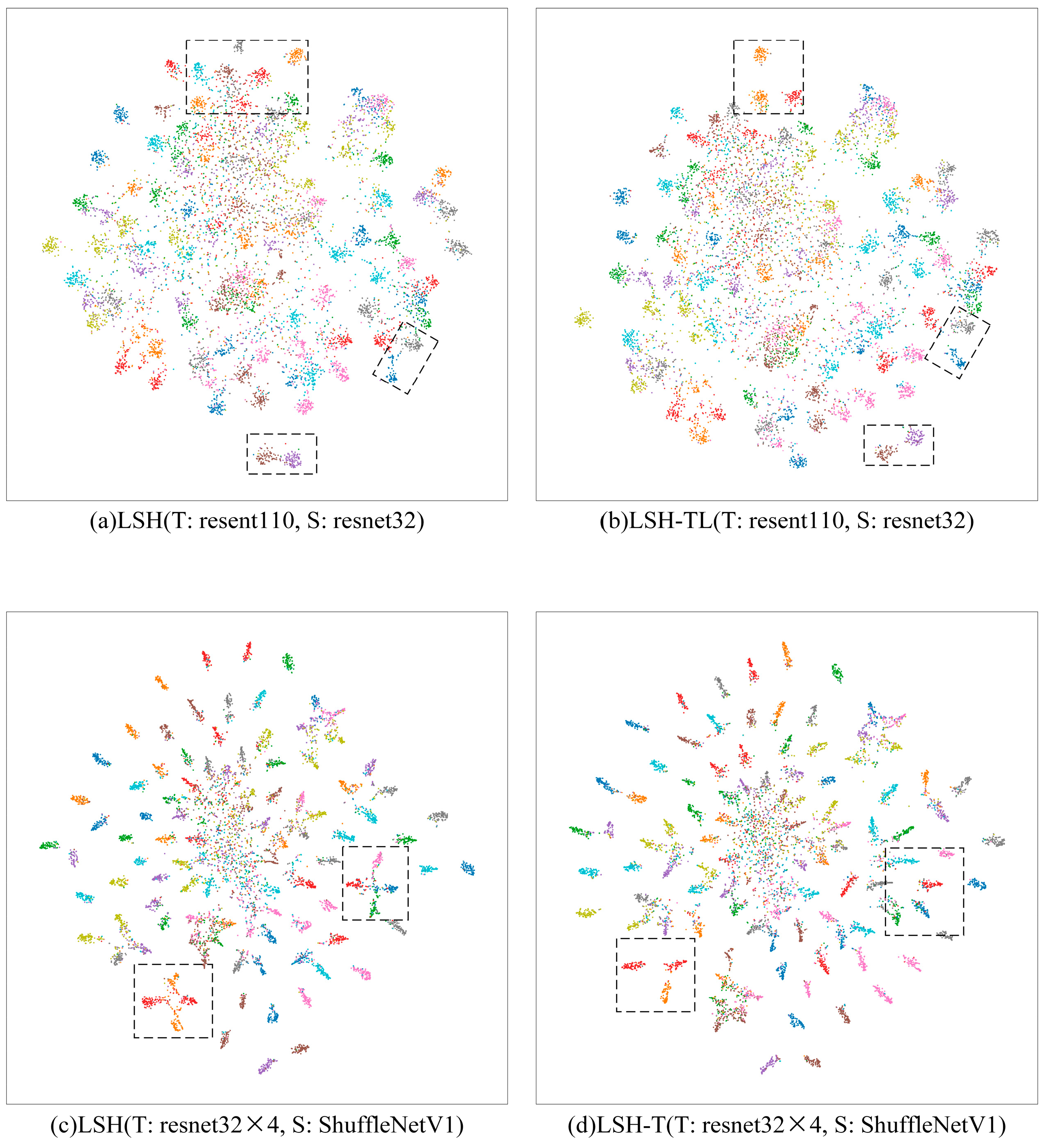
We carried out the visualization of the features in the penultimate layer of the model using the t-SNE algorithm (t-distributed Stochastic Neighbor Embedding) (on the Cifar-100 dataset, with resnet110 and resnet32×4 for teachers and resnet32 as well as shufflenetv1 for students).
In the t-SNE results, we can observe whether data points of different categories can be separated in space, and judge whether the model has effectively learned the features and structure of the data. In general, we want data points of different categories to be separated in the graph. Data points of the same category are as close to each other as possible, while data points of different categories are clearly bound or spaced apart.
In Figure 6, we have enclosed with dashed boxes some of the places where LSH-TL and LSH-T perform better relative to the original LSH for penultimate layer feature separation. The t-SNE results show that representations of LSH-TL and LSH-T are more separable than LSH.
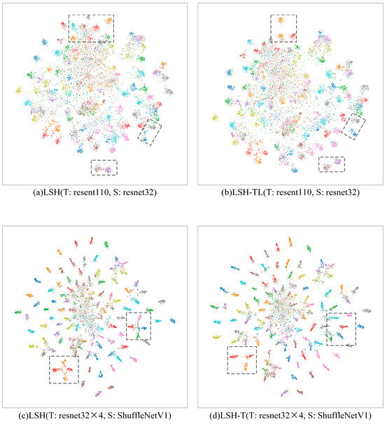
Figure 6.
t-SNE of penultimate layer features learned by LSH, LSH-TL, and LSH-T. T stands for the teacher model and S for the student model for distillation. Each color represents a class of feature output.
4.5. Discussion on Results
Despite the improvement in performance compared to LSH, our algorithm still performs slightly worse than SSKD in heterogeneous model distillation. This can be attributed to two reasons. First, there are differences in the penultimate dimension between teachers and students in heterogeneous model distillation. The feature output of a heterogeneous teacher is less helpful to the student than that of a homogeneous teacher. Secondly, because the SSKD self-supervised image enhancement method increases the amount of data and requires pre-training of the teacher self-supervision module, the SSKD training time is longer. In contrast, as shown in Table 8, our algorithms have a shorter training time and lower memory usage.
Table 8.
Comparison of SSKD, LSH-TL, and LSH-T on training time and memory usage.
In Section 4.2 and Section 4.3, we conducted ablation experiments on LSH-TL and LSH-T, respectively. Although these two algorithms cannot be utilized together, the experiments indicate that they have distinct application scenarios. At the same time, we summarize the underlying reasons for the excellent performance of LSH-TL and LSH-T:
The superior performance of LSH-TL and LSH-T compared to other algorithms in homogeneous and heterogeneous model distillation is the effectiveness of the penultimate layer of features as knowledge. The model penultimate layer features are derived from the output of the backbone network features after pooling. Compared with other knowledge distillation algorithms based on intermediate layer features, the advantage is that more layers of neural networks process the penultimate layer features, and the amount of information contained is richer. As opposed to logits distillation, students prioritize learning the mapping parameters (weights and biases) of the penultimate layer to the classification layer to fit the teacher output logits, instead of fitting the backbone network output features. The advantage of penultimate layer feature distillation is that the pooling operation has no updatable parameters. Students need to fit the teacher’s penultimate layer features to fit the teacher’s backbone network feature output at the same time. The students can learn the teacher’s feature outputs from all parts of the teacher in a better way. LSH-TL and LSH-T further address the need for students in knowledge distillation to learn the data distribution of images in real task scenarios by further fitting the training data to the ground-truth distribution of images based on classes and features.
LSH-TL enhances the penultimate layer feature distillation performance of both homogeneous and heterogeneous models by employing teacher labels instead of dataset one-hot labels to supervise student classification. This adjustment allows the student classification output to better align with the ground-truth distribution of classes. Due to the unique residual structure of the resnet [2], the deep resnet model is built upon the shallow resnet model. It is likely that the deep resnet model outperforms the shallow resnet model under similar training conditions. Therefore, the teacher label generated by the deep resnet model is beneficial for training the shallow resnet model. Therefore, LSH-TL is suitable for distilling resnet models with similar architectures. Moreover, LSH-TL compensates for the limitation of LSH-T, which cannot be applied to resnet model distillation.
LSH-T is applied to adjust the teacher’s penultimate layer feature output by introducing feature temperatures, aiming to align it with the ground-truth distribution of features. The LSH-T algorithm performs better when the penultimate layer feature output of the teacher model is relatively low. Vgg13, resnet32×4, and WRN-40-2 fit the application scenario when used as teacher models for feature distillation. However, when using resnet base models as teachers, the feature output values in their penultimate layer are in the normal range, resulting in poor performance of the LSH-T algorithm.
5. Conclusions
In this paper, we argued that the existing work on penultimate layer feature distillation overlooked the efforts focused on fitting the ground-truth distribution of the image. To address this issue, we proposed two penultimate layer feature distillation algorithms LSH-TL and LSH-T.
LSH-TL focuses on fitting the ground-truth distribution based on classification. It supervises the classification output by replacing the traditional dataset labels with teacher classification labels that are more consistent with the ground-truth distribution of classes; LSH-T corrects the low-feature output distribution of the teacher by designing the feature temperature. Make the teacher feature output distribution more consistent with the ground-truth distribution of features. On the Cifar-100 dataset, LSH-TL outperforms the base LSH in nine out of a total of thirteen homogeneous and heterogeneous distillation model groups, providing a maximum performance gain of 0.17% for LSH. LSH-T outperforms the base LSH in eight out of a total of thirteen homogeneous and heterogeneous distillation model groups, providing a maximum performance gain of 0.60% for LSH. The two methods have their application areas and compensate for each other’s shortcomings. LSH-TL can provide a performance gain effect in the three-group homogeneous model of resnet where LSH-T distillation performance is poor. LSH-T can also obtain good distillation performance results on distillation teacher–student groups such as vgg13–vgg8 where LSH-TL performance is not satisfactory. Experimental results on the large dataset ImageNet-2012 show that LSH-TL and LSH-T are lower than the original LSH algorithm in both Top-1 and Top-5 error rates. These experimental results validate the effectiveness of our ground-truth distribution fitting approach.
Our work still has some limitations. In LSH-TL, it is hard to eliminate the effect of teacher output mislabeling on the distillation performance of the algorithm. In LSH-T, the characteristic temperature parameters need to be set manually, which makes it difficult to select the optimal parameters for all distillation model groups. And, the distillation performance is not good after the fusion of the two methods.
Teacher output mislabeling affects the performance of the LSH-TL algorithm because teacher labels are used in LSH-TL to supervise student classification output. Students’ judgment is poor when their performance is low, and students will receive all of the teacher’s output mislabels, causing them to learn the wrong knowledge and affecting the algorithm’s distillation performance. To address this issue, future work will explore how to incorporate more efficient supervised approaches such as self-supervised learning to compensate for the problem of teachers outputting incorrect labels. In the following works, we will explore more ways to improve our algorithms, such as incorporating a dynamic search for optimal intervals for feature temperature parameters, and combining the two algorithms into one to become a more adaptable algorithm.
Author Contributions
Conceptualization, J.L. and Z.T.; methodology, J.L.; software, J.L.; validation, J.L., K.C. and Z.C.; formal analysis, J.L.; investigation, J.L.; resources, Z.T.; data curation, J.L.; writing—original draft preparation, J.L.; writing—review and editing, J.L. and Z.T.; visualization, J.L. and K.C.; supervision, Z.T.; project administration, Z.T.; funding acquisition, Z.T. All authors have read and agreed to the published version of the manuscript.
Funding
This work was supported by the National Natural Science Foundation of China under grant 62171145 and by the Guangxi Natural Science Foundation under Grant 2021GXNSFAA220058.
Institutional Review Board Statement
Not applicable.
Informed Consent Statement
Not applicable.
Data Availability Statement
The original contributions presented in the study are included in the article, further inquiries can be directed to the corresponding author.
Conflicts of Interest
The authors declare no conflicts of interest.
References
- Ma, N.; Zhang, X.; Zheng, H.T.; Sun, J. Shufflenet v2: Practical guidelines for efficient cnn architecture design. In Proceedings of the European Conference on Computer Vision (ECCV), Munich, Germany, 8–14 September 2018; pp. 116–131. [Google Scholar]
- He, K.; Zhang, X.; Ren, S.; Sun, J. Deep residual learning for image recognition. In Proceedings of the IEEE Conference on Computer Vision and Pattern Recognition, Las Vegas, NV, USA, 27–30 June 2016; pp. 770–778. [Google Scholar]
- Hu, J.; Shen, L.; Sun, G. Squeeze-and-excitation networks. In Proceedings of the IEEE Conference on Computer Vision and Pattern Recognition, Salt Lake City, UT, USA, 18–23 June 2018; pp. 7132–7141. [Google Scholar]
- He, K.; Gkioxari, G.; Dollár, P.; Girshick, R. Mask r-cnn. In Proceedings of the IEEE International Conference on Computer Vision, Venice, Italy, 22–29 October 2017; pp. 2961–2969. [Google Scholar]
- Ren, S.; He, K.; Girshick, R.; Sun, J. Faster R-CNN: Towards real-time object detection with region proposal networks. IEEE Trans. Pattern Anal. Mach. Intell. 2016, 39, 1137–1149. [Google Scholar] [CrossRef] [PubMed]
- Redmon, J.; Divvala, S.; Girshick, R.; Farhadi, A. You only look once: Unified, real-time object detection. In Proceedings of the IEEE Conference on Computer Vision and Pattern Recognition, Las Vegas, NV, USA, 27–30 June 2016; pp. 779–788. [Google Scholar]
- Ronneberger, O.; Fischer, P.; Brox, T. U-net: Convolutional networks for biomedical image segmentation. In Proceedings of the Medical Image Computing and Computer-Assisted Intervention—MICCAI 2015: 18th International Conference, Munich, Germany, 5–9 October 2015; Proceedings, Part III 18; Lecture Notes in Computer Science. Springer International Publishing: Cham, Switzerland, 2015; pp. 234–241. [Google Scholar]
- Zhao, H.; Shi, J.; Qi, X.; Wang, X.; Jia, J. Pyramid scene parsing network. In Proceedings of the IEEE Conference on Computer Vision and Pattern Recognition, Honolulu, HI, USA, 21–26 July 2017; pp. 2881–2890. [Google Scholar]
- Long, J.; Shelhamer, E.; Darrell, T. Fully convolutional networks for semantic segmentation. In Proceedings of the IEEE Conference on Computer Vision and Pattern Recognition, Boston, MA, USA, 7–12 June 2015; pp. 3431–3440. [Google Scholar]
- Hinton, G.; Vinyals, O.; Dean, J. Distilling the knowledge in a neural network. arXiv 2015, arXiv:1503.02531. [Google Scholar]
- Romero, A.; Ballas, N.; Kahou, S.E.; Chassang, A.; Gatta, C.; Bengio, Y. Fitnets: Hints for thin deep nets. arXiv 2014, arXiv:1412.6550. [Google Scholar]
- Tian, Y.; Krishnan, D.; Isola, P. Contrastive representation distillation. arXiv 2019, arXiv:1910.10699. [Google Scholar]
- Wang, G.H.; Ge, Y.; Wu, J. Distilling knowledge by mimicking features. IEEE Trans. Pattern Anal. Mach. Intell. 2021, 44, 8183–8195. [Google Scholar] [CrossRef] [PubMed]
- Xu, K.; Rui, L.; Li, Y.; Gu, L. Feature normalized knowledge distillation for image classification. In Proceedings of the European Conference on Computer Vision, Glasgow, UK, 23–28 August 2020; Springer: Cham, Switzerland, 2020; pp. 664–680. [Google Scholar]
- Frénay, B.; Verleysen, M. Classification in the presence of label noise: A survey. IEEE Trans. Neural Netw. Learn. Syst. 2013, 25, 845–869. [Google Scholar] [CrossRef] [PubMed]
- Zhao, B.; Cui, Q.; Song, R.; Qiu, Y.; Liang, J. Decoupled knowledge distillation. In Proceedings of the IEEE/CVF Conference on Computer Vision and Pattern Recognition, New Orleans, LA, USA, 18–24 June 2022; pp. 11953–11962. [Google Scholar]
- Zagoruyko, S.; Komodakis, N. Paying more attention to attention: Improving the performance of convolutional neural networks via attention transfer. arXiv 2016, arXiv:1612.03928. [Google Scholar]
- Heo, B.; Lee, M.; Yun, S.; Choi, J.Y. Knowledge transfer via distillation of activation boundaries formed by hidden neurons. In Proceedings of the AAAI Conference on Artificial Intelligence, Honolulu, HI, USA, 27 January–1 February 2019; pp. 3779–3787. [Google Scholar]
- Tung, F.; Mori, G. Similarity-preserving knowledge distillation. In Proceedings of the IEEE/CVF International Conference on Computer Vision, Seoul, Republic of Korea, 27 October–2 November 2019; pp. 1365–1374. [Google Scholar]
- Yim, J.; Joo, D.; Bae, J.; Kim, J. A gift from knowledge distillation: Fast optimization, network minimization and transfer learning. In Proceedings of the IEEE Conference on Computer Vision and Pattern Recognition, Honolulu, HI, USA, 21–26 July 2017; pp. 4133–4141. [Google Scholar]
- Kim, J.; Park, S.U.; Kwak, N. Paraphrasing complex network: Network compression via factor transfer. Adv. Neural Inf. Process. Syst. 2018, 31. [Google Scholar]
- Xu, G.; Liu, Z.; Li, X.; Loy, C.C. Knowledge distillation meets self-supervision. In Proceedings of the European Conference on Computer Vision, Glasgow, UK, 23–28 August 2020; Springer International Publishing: Cham, Switzerland, 2020; pp. 588–604. [Google Scholar]
Disclaimer/Publisher’s Note: The statements, opinions and data contained in all publications are solely those of the individual author(s) and contributor(s) and not of MDPI and/or the editor(s). MDPI and/or the editor(s) disclaim responsibility for any injury to people or property resulting from any ideas, methods, instructions or products referred to in the content. |
© 2024 by the authors. Licensee MDPI, Basel, Switzerland. This article is an open access article distributed under the terms and conditions of the Creative Commons Attribution (CC BY) license (https://creativecommons.org/licenses/by/4.0/).