Abstract
This study aims to optimize the Weather Research and Forecasting (WRF) model regarding the choice of the best planetary boundary layer (PBL) physical scheme and to evaluate the model’s performance for wind energy assessment and mapping over the Iranian territory. In this initiative, five PBL and surface layer parameterization schemes were tested, and their performance was evaluated via comparison with observational wind data. The study used two-way nesting domains with spatial resolutions of 15 km and 5 km to represent atmospheric circulation patterns affecting the study area. Additionally, a seventeen-year simulation (2004–2020) was conducted, producing wind datasets for the entire Iranian territory. The accuracy of the WRF model was assessed by comparing its results with observations from multiple sites and with the high-resolution Global Wind Atlas. Statistical parameters and wind power density were calculated from the simulated data and compared with observations to evaluate wind energy potential at specific sites. The model’s performance was sensitive to the horizontal resolution of the terrain data, with weaker simulations for wind speeds below 3 m/s and above 10 m/s. The results confirm that the WRF model provides reliable wind speed data for realistic wind energy assessment studies in Iran. The model-generated wind resource map identifies areas with high wind (wind speed > 5.6 m/s) potential that are currently without wind farms or Aeolic parks for exploitation of the wind energy potential. The Sistan Basin in eastern Iran was identified as the area with the highest wind power density, while areas west of the Zagros Mountains and in southwest Iran showed high aeolian potential during summer. A novelty of this research is the application of the WRF model in an area characterized by high topographical complexities and specific geographical features. The results provide practical solutions and valuable insights for industry stakeholders, facilitating informed decision making, reducing uncertainties, and promoting the effective utilization of wind energy resources in the region.
1. Introduction
Environmental issues such as the changing climate and global warming are a major concern, especially as energy demand continues to rise globally [1,2]. Consumer responses to energy markets change with economic development, as energy is consumed to meet the increasing demands for energy services. This longer-term perspective offers insights into the evolution of energy service use and energy markets, providing valuable empirical evidence for developing climate policies over extended timescales [3]. Raising regional and country-level ambitions will be crucial to meet interlinked energy and climate objectives, especially in the urban environment [4,5]. New, clean and renewable energy resources are vital to meet this demand and to tackle environmental issues [6]. Wind energy is one of the cleanest and most accessible energy sources that can respond to the world’s energy demands, and its contribution to the electricity supply is significantly increasing worldwide [7]. Significant changes have occurred in the outlook for renewable energy sources over the past decade. Renewable energy, once an emerging trend, has become a global necessity, and it experienced an unprecedented growth in global electricity production in 2021, despite the major challenges posed by the COVID-19 pandemic and the unprecedented increase in the global price of energy and commodities. Therefore, for the first time ever, solar and wind energy provided more than 10% of the world’s electricity [8]. In 2022, the wind industry had its third-best year, and the dual challenge of secure energy supply and climate goals will propel wind power into a new phase of extraordinary growth, with the demand for wind energy continuing to expand in many countries [7,9]. The global share of renewable electricity production must increase to 28% by 2030 and 66% by 2050 to limit the increase in global average temperature to less than 2 °C by the end of the century [5]. To achieve this purpose, providing accurate wind data, especially in developing countries, is one of the basic priorities, while the assessment of the wind energy potential is highly important.
About 25 years ago, in Iran, the establishment of an organization dedicated to the development of renewable energy signaled a commitment to strategic planning and concerted efforts to access relevant data and technologies. Presently, the Renewable Energy and Energy Efficiency Organization (SATBA) is entrusted with the responsibilities of identifying renewable energy resources, undertaking strategic planning and facilitating their development. Since around 2015, this organization has actively pursued private sector engagement and market stimulation, employing mechanisms such as “Feed-in Tariffs (FIT)” and implementing “Power Purchase Agreements (PPA)”. In Iran, a country rich in fossil energy resources, the exploration of new energy methods and resources necessitates a pragmatic approach. By the year 2018, approximately 12 wind farms with capacities ranging from about 1.5 to 61.2 MW had been established [10].
High-quality wind data are essential for a comprehensive wind energy assessment process [9]. To evaluate the wind energy potential over an area, accurate wind data at typical turbine hub heights is necessary. In general, at least one year of collected data are required to realistically estimate the wind energy production potential of a given area [11,12]. Such data could be collected by installing wind masts to measure wind speed at different heights. However, installing and operating wind masts are very expensive and time-consuming practices [5]. An alternative approach involves utilizing wind measurements obtained from meteorological stations within a dense network, which are typically taken at a height of 10 m above ground level (a.g.l.). Subsequently, these near-surface wind data can be extrapolated to standard hub heights by applying power or logarithmic laws [13,14,15]. However, such methods are based on assumptions about the boundary layer height and dynamics, as well as the atmospheric stability and clouds, which are not always true and can lead to considerable biases in the wind energy potential estimation [16,17]. The WRF model is one of the most commonly widely used meteorological models for simulating the wind regime and for wind resource assessment studies [18,19,20,21]. Minimizing errors in wind simulation involves testing and selecting an appropriate numerical and physical configuration tailored to the specific region of interest, along with the utilization of high-resolution terrain data, when accessible [22]. WRF was used to simulate the planetary boundary layer over the period 2011 to 2015, aiming to assess the wind resources in eastern Iran [23]. Wind simulations via the WRF model have been used in many studies to investigate dust rising, transportation and propagation in the Middle East [24,25,26,27]. Furthermore, several studies have employed numerical models in the evaluation of the wind energy resources in various areas around the world [28,29,30,31].
Nonetheless, there are several sources of errors and uncertainty in numerical model simulations, such as the representation of sub-grid physical processes (like the ones related to the surface layer, SL, and the planetary boundary layer, PBL) that cannot be explicitly resolved by the models [17,32]. To consider these processes in numerical weather prediction (NWP) models, some assumptions and approximations are included in the models that allow them to implicitly represent these unresolved processes, called physical parametrizations. WRF is a complex model containing some numerical, dynamical and physical options that can be individually chosen by the user [33,34,35]. The choice of a given set of physical parameterizations can have a significant impact in wind simulation and wind energy estimation over a given area. Several studies have dealt with the evaluation of the sensitivity of the WRF model to make the choice of PBL parameterizations in wind simulations [36,37,38,39,40,41,42,43,44,45,46,47]. These studies revealed that the simulation of the wind field is sensitive to the physical parameterization’s selection, and that the performance of these parameterizations vary significantly according to the studied geographical region, highlighting the need to carry out sensitivity studies to determine the optimal model configuration for the simulation of the wind regime in a specific area.
Iran is currently very dependent on fossil fuels in terms of its energy demand and economic exports [48,49,50]. So, under a climate change scenario in the Middle East [51,52], in the future, Iran will have to implement renewable energy systems for the purposes of covering increased energy demands. The need for wind energy resource assessment in various parts of Iran has gained growing importance, aiming to expand the country’s energy resources and to reduce fossil fuel consumption [48,53,54]. For this issue, sources of accurate wind data are very crucial. Initial studies using wind measurements revealed that Iran has an attractive wind energy potential [55,56]. However, because of the country’s vastness and the lack of consistent wind measurement campaigns, and/or a dense meteorological network for wind measurements in remote areas of the country, it is presently very difficult to map the areas of the country with exploitable wind energy potential. Therefore, the use of NWP simulated data is an inevitable necessity, and the most significant gap in this issue is the lack of evaluation of the performance of different model schemes, as well as the absence of long-term simulations of wind fields in this vast and highly complex topographic region. This subject has received little attention so far, and only a limited number of studies have been conducted using NWP models to evaluate the wind energy potential in Iran [45], while all studies focused on the eastern part of the country [57,58]. So, the current results shed light to the important role of evaluating the best WRF model configuration for wind energy resource assessment and mapping in Iran.
The main goals of this study are to generate wind climate data at different levels in the lower troposphere over Iran and to prepare a mesoscale wind energy map via the WRF model over a long period, in a region with a very complex topography. In addition, this study aims to identify areas with high wind energy production potential, and to provide an initial assessment of the amount of wind energy that can be extracted, as well as the necessary data for the study and development of small-scale wind farms in the identified areas. Under a warmer world scenario and with the temperature increase in the Middle East in the coming decades to be much higher than the global average [52], the transition from fossil fuels to renewable energy sources is more than imperative.
In an area with a great lack of observational data, the most important step to achieve this goal is to optimize the WRF model for wind energy assessment and spatial mapping, and mainly to evaluate the choice of the SL and PBL parameterizations in the model that better represent the wind regime over the country. This is one of the first studies that used NWP models to evaluate the wind energy potential throughout the Iranian territory. For this purpose, different physical configurations of the WRF model were evaluated and the best configuration was obtained for wind simulations over Iran. Then, a 17-year climate wind dataset was generated, enabling the identification of high-potential wind energy areas throughout the country and providing the basis for further studies to prepare micro-scale data for the establishment of wind farms.
2. Materials and Methods
2.1. Study Area, Data and Wind Measuring Stations
The study domain covers the whole Iranian territory, with an area of approximately 1,648,195 km², while over the half is mountainous terrain (Figure 1). Iran is known for its rugged topography, featuring high mountains, deep valleys, extensive arid basins, vast desert areas, and topographic low drainage basins [59]. The arid and semi-arid terrain is particularly vulnerable to land degradation and wind erosion, especially during spring and summer, when vegetation coverage is low and the winds are stronger [60,61,62,63]. The topography of the study area can be broadly characterized as a great plateau (Central Iranian Plateau, Kavir and Lut Deserts) surrounded by two high mountainous ranges (see Figure 1). The Alborz Mountains in the north have a long east–west axis with peaks exceeding 3000 m in height, and some reaching over 5000 m. In the west and southwest, the Zagros Mountains extend over a vast distance, with most areas being over 1800 m in elevation, and many summits exceeding 3600 m. The great central plateau, rising to about 1000 m above sea level (asl), dominates most of the country, while some parts, such as the Lut valley and the Sistan Basin, are only around 500 m asl.
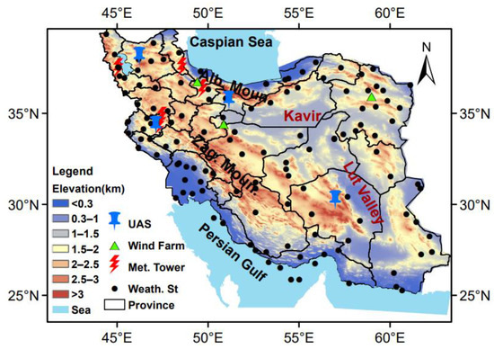
Figure 1.
The study area and the location of the wind farms, weather stations, meteorological towers (Met. Tower) and upper air stations (UAS) in the Iranian territory.
Figure 1 also displays the locations of the stations used in this study, including weather stations, upper air stations, meteorological towers, and operational wind farms. This study utilized four available datasets to verify and compare the model results with observational data. These datasets included:
- (i)
- Ten-meter wind data in meteorological stations: In order to comprehensively assess the model results, we selected 140 weather stations distributed across the country. After conducting quality control on the synoptic data, we narrowed down our selection to 110 stations (as shown in Figure 1) that had complete data available from 2004 to 2020, which were then compared with the wind simulations generated by the model.
- (ii)
- Data from upper air stations (UAS): The studied area comprises approximately 10 UAS. However, these stations are not operational on a continuous basis and often have gaps in their data records. Most of these stations conduct observations at specific times, either at 00 UTC or 1200 UTC. Additionally, the available data from these stations had a time step of 10 s, and the stations did not provide wind data at heights near the ground surface for model verification purposes. Fortunately, data with a time step of 2 s were successfully extracted from four UAS (as shown in Figure 1) for the months of January and July 2013, which were then utilized for verifying the model results.
- (iii)
- Meteorological mast data: Data from five meteorological masts (Figure 1) were utilized to verify the model results.
- (iv)
- Available data from the Global Wind Atlas: To compare the simulated wind results with those from The Technical University of Denmark (DTU) Wind Atlas, data from 2008 to 2017 were used.
2.2. Model Description
This study made use of the Advanced Research WRF model (ARW) version 3.9.1, which is a limited area model (LAM) featuring a state-of-the-art atmospheric modelling system designed for both meteorological research and numerical weather prediction [64,65]. LAMs are widely used for providing weather forecasts beyond three days, with a forecast skill ranging between 80% and 90% [66]. For this study, wind data were obtained by analyzing the WRF mesoscale model simulations for wind energy resource assessment in Iran over a 17-year period (2004–2020).
2.3. Model Setup
This study utilized two-way nesting domains with spatial resolutions of 15 km (D1) and 5 km (D2), as shown in Figure 2. D1 was wide enough to cover the atmospheric circulation synoptic systems that affect the study area. The model defined thirty-nine vertical levels from the surface up to the 100 hPa pressure level. The ECMWF (European Centre for Medium-Range Weather Forecasts) Era-Interim data with 0.75° spatial horizontal resolution every 6 h were used to derive the initial and boundary conditions. Terrestrial data required for the model, including land use, land mask, albedo, and topography, were obtained from the USGS (United States Geological Service) database.
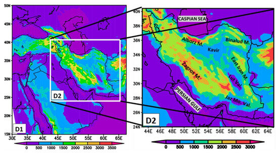
Figure 2.
The two defined domains in the WRF model simulations over Iran. The colored scale corresponds to altitude (m). M, Mo and Val stand for the words Mountain, Mourian and Valley, respectively. The designations D1 and D2 refer to the WRF Model Domains. D1 represents the parent domain, covering the Middle East and surrounding areas, while D2 represents the smaller domain specifically focusing on Iran. The data from D2 was utilized in creating the wind atlas.
The nudging coefficients in WRF were set to a default value of 3.0 × 10⁻⁴ s−1 for each variable. These values were derived from observation-driven studies that used analysis nudging in WRF’s predecessors, MM4 and MM5 [67,68]. In essence, the nudging coefficients represent the reciprocal time scales of the physical processes in the data that the model is nudged towards.
The nudging technique can reduce the error of dynamic downscaling simulations and improve the consistency with the driving data [69]. Since dynamical downscaling results usually drift away from large-scale synoptic driving fields, the nudging in domain 1 can be used to balance the performance of dynamical downscaling at large and small scales. Therefore, analysis nudging was used for domain 1 and above the boundary layer for the wind, temperature and specific humidity. Nudging was used to relax the model solution toward the analysis data, and it was proven to be effective in reducing the wind speed error [70,71].
To ensure that the initial conditions were applied every 48 h, the WRF model was restarted at 00 UTC every 48 h. The first 12 h of each simulation were excluded from the analysis since they account for the model spin-up.
To estimate the WRF performance in the simulation of the wind field, a preliminary evaluation was carried out with a model-to-data comparison using five SL and PBL parameterization schemes during cold (January) and warm (July) months in 2013. For this purpose, the simulated wind speed by the model was compared with the wind data obtained by the upper air sounding. Comparisons were performed at 4 heights of 10, 40, 80 and 100 m, considering the sensitivity of each of the parameterizations to the environmental conditions and the stability of the atmosphere. Among the 13 active upper air stations throughout the country, 4 stations (Tehran, Kerman, Kermanshah and Tabriz) had suitable data (wind data below 100 m) for comparison with the model output. Table 1 shows the characteristics of these 4 upper air observation stations.

Table 1.
The coordinates of the 4 upper air observation stations, the height of the model grids and their height differences within the stations. Hs and Hm represent the heights (above sea level) of the observation stations and model grids, respectively, and D is their difference.
The wind resource maps were developed by simulating weather conditions from a large number of days and for a long-term period [72]. Therefore, after obtaining the best configuration, a long-term simulation over a seventeen-year period (2004–2020) was carried out and a wind dataset with one-hour time steps was prepared for 1,584,840 grid points covering the whole Iranian territory. Then, the calculated average wind speeds for all the grid points were summarized to develop the annually, seasonally and monthly wind maps at different heights. Table 2 shows the details of WRF configuration, including the model parameterization schemes that were used in the simulations.
Table 2.
Summary of WRF model setup used for the simulations in this study.
2.4. Sensitivity Analysis
The PBL schemes implemented in the WRF model are divided into two categories, local and non-local schemes. Since their performance depends on the geographical area under study and the prevailing atmospheric conditions, it cannot be identified with certainty that a given PBL scheme fits better than others for every geographical region in a general sense [76].
In this study, five different PBL schemes were tested to assess which one allows the best simulation of the wind field over the whole of Iran. The five PBL schemes tested here were: (i) Yonsei University (YSU) [77,78], (ii) Mellor, Yamada and Janjić (MYJ) [79,80], (iii) Mellor–Yamada–Nakanishi–Niino (MYNN2.5) [81], (iv) Quasi-Normal Scale Elimination (QNSE) [82], and (v) Asymmetric Convective Model Version 2 (ACM2) [83].The PBL schemes aim to capture the exchange of heat, moisture, and momentum between the surface and the atmosphere. Below, a brief overview of the five PBL schemes and their differences is given:
- (i)
- The YSU scheme is widely utilized for its ability to handle a diverse range of atmospheric conditions. It employs a non-local closure approach and incorporates both local and non-local mixing processes within the boundary layer. The YSU scheme’s notable feature is its use of a prognostic equation for turbulent kinetic energy.
- (ii)
- The MYJ scheme combines elements of local and non-local closures and adopts an eddy diffusivity approach to represent turbulent mixing. This scheme also includes a counter-gradient term to account for buoyancy effects.
- (iii)
- The MYNN2.5 scheme is an advanced extension of the MYJ scheme, aiming to enhance the representation of the vertical structure of the boundary layer. It introduces additional prognostic equations for turbulent kinetic energy and incorporates a higher-order closure for sub-grid-scale turbulence.
- (iv)
- QNSE Scheme: In contrast to the previous schemes, the QNSE scheme adopts a different approach based on quasi-normal scale elimination. It explicitly solves equations for turbulent kinetic energy and its dissipation rate, allowing for a more precise representation of boundary layer processes. The QNSE scheme effectively captures the effects of both local and non-local turbulent mixing.
- (v)
- ACM2 Scheme: Designed specifically for weather and climate prediction models, the ACM2 scheme focuses on representing convective processes within the boundary layer. It employs a multi-plume approach to simulate convective updrafts and downdrafts, enabling a more realistic representation of convective phenomena.
In summary, these PBL schemes differ in their approaches, equations, complexity, and focus. The YSU, MYJ, and MYNN2.5 schemes employ a combination of local and non-local closures, whereas the QNSE scheme utilizes quasi-normal scale elimination. The ACM2 scheme emphasizes the representation of convective processes. The schemes also vary in the number of equations that they solve, with the MYNN2.5 and QNSE schemes being more advanced and computationally demanding. Ultimately, the choice of PBL scheme depends on the specific modeling requirements and the atmospheric conditions being simulated. Each scheme has its own strengths and limitations, and the selection should be made based on the intended application and the desired balance between accuracy and computational efficiency.
In numerical models, the representation of turbulent motions in the atmosphere depends on two processes in PBL schemes: (i) considering a local or non-local mixing approach and (ii) the order of turbulence closure. Among the five schemes that were investigated, the YSU scheme is a first order non-local scheme adapted from the Medium Range Forecast (MRF) boundary layer scheme. The YSU scheme uses the K-profile approach to parameterize turbulent mixing. The MYJ scheme is a local 1.5-order scheme and a modified version of the original Mellor and Yamada [79] level 2.5 and level 2 models developed by Janjić [80] that uses a revised master length scale. The MYNN is a local 1.5-order scheme and is the modification of the MY scheme, similar to MYJ. The MYNN scheme uses large eddy simulation (LES) for the purposes of solving pressure-temperature-gradient covariance and pressure strain that are neglected by the MY scheme. QNSE is also a local 1.5-order scheme, although there are some differences compared to the other schemes. ACM2 is a first-order scheme and asymmetrical convection model, version 2. The ACM2 treats both non-local large-scale transportations, as well as local sub-grid scale diffusion.
In this study, the simulation contained two two-way nested domains with horizontal resolutions of 15 km and 5 km, for D1 and D2, respectively (Figure 2). The following analysis to evaluate the model performance and wind energy resource assessment was carried out for the inner domain (D2).
2.5. Verification of the Model Results
In this study, we evaluated the accuracy of the WRF model by comparing its results with observations from multiple sites and the high-resolution Global Wind Atlas (GWA). To ensure that the model results were consistent with the real wind conditions across Iran, we gathered wind observations from three sources: (i) synoptic weather stations, (ii) upper air stations, and (iii) meteorological masts installed by the SATBA at five locations across the country (as listed in Table 3). The wind masts recorded wind data every ten minutes at three different heights, while the weather stations recorded wind data every three hours at a height of 10 m a.g.l. Common statistical parameters were used to evaluate the model’s performance.
Table 3.
Summary of the wind masts in Iran used for evaluation of the WRF model performance.
- (1)
- Information regarding temporal co-variability is provided here through the root mean square error (RMSE), which estimates systematic biases in the model skill, aswhere “y” is the simulated wind speed, “o” is the wind speed observation at the same place and time, and “n” is the total number of the values’ pairs.
- (2)
- “Bias” is a common statistical error for comparing the wind speed distribution between observations and model simulations.
If the mean Bias is positive, the simulated values tend to overestimate the real values and vice versa.
- (3)
- The Standard Deviation Error (STDE),
The STDE is very useful to evaluate the error dispersion. The low STDE value indicates that the error can be related to a source other than the simulation physics [17]. Therefore, priority is given to this quantity.
2.6. Wind Energy Production Estimation
In this study, the wind regime over Iran was simulated via the WRF model for a long period (2004–2020), while the year 2013 was used for the evaluation of the PBL results due to the greater availability of upper air sounding data. To evaluate the wind energy potential at a specific site, statistical parameters (mean and median) and wind power density (WPD) were calculated from the simulated data and compared with the observations. Among various methods for the investigation and statistical distribution of wind speed data, the Weibull distribution function is widely known as the most suitable function due to its simplicity and high accuracy [84]. The WPD in terms of Weibull probability density function was calculated as
where C is the Weibull scale parameter (m/s), ρ is the air density (1.225 Kg m−3), K is the Weibull shape parameter (dimensionless), and Γ is the gamma function.
The wind energy potential at a specific site can be estimated through the analysis of the Weibull distribution, and the model performance in simulating the wind can also be evaluated by comparing observed and simulated Weibull distributions [54,85,86,87].
3. Results and Discussion
3.1. Sensitivity Analysis
In numerical modelling studies, evaluating the simulations with the available data supports the performance of the selected model configuration [32]. Therefore, based on this principle, this section presents the results of the WRF sensitivity analysis due to the use of five different PBL schemes. The first step is to determine which set of physical options (parameterizations) leads to the best results (lower error and uncertainty) for a winter and a summer month. Here, only the weighted mean values (i.e., the mean for all mast stations weighted by the number of data records) of each statistical parameter were presented at each height.
The RMSE, Bias and STDE values between measured and simulated wind data at the heights of 10, 40 and 80 m for January 2013 are presented in Table 4. These statistical indicators were calculated for pairs of simultaneous and valid records of simulations and observations. According to this table, the QNSE PBL scheme is that with the lowest errors for January 2013, with Bias, RMSE and STDE values equal to 0.78, 4.14 and 4.05 (m/s), respectively. Given the higher-ranking criterion of the STDE over the RMSE and Bias, it is concluded that after the QNSE, the ACM2 configuration presented the best performance (STDE = 4.07 m/s). Overall, a positive bias was determined, indicating that the WRF model consistently overestimates the wind speed regardless of the PBL scheme. This observation highlights the presence of systematic biases in model simulations over complex terrain regions such as deep valleys and mountain tops. However, the simulation biases may vary highly between the stations and some of them may also indicate a model underestimation, as was seen for the case of Fadeshk meteorological tower (Supplementary Material).
Table 4.
Statistical parameters calculated from the comparison between the model outputs and wind observations at mast stations for different PBL schemes in January 2013.
According to Table 5, the statistical results of the comparison obtained for July 2013 were relatively different from those of January 2013. The best performance was presented for the ACM2 configuration with Bias, RMSE and STDE equal to 0.6, 3.4 and 3.22, respectively. The QNSE PBL scheme, which showed the best performance in the cold season, revealed the highest errors in the warm season (with STDE = 3.65). Similar to what was seen in the cold season, all simulations showed a tendency to overestimate the wind speed in summer as well. In general, the error values were lower in July than in January, indicating a better model performance in summer. However, all PBL schemes indicate rather small differences in the statistical indicator values (Bias, RMSE, STDE) in both cold and warm months, resulting in a challenge in detecting the best scheme for model simulations of wind climatology in Iran. It should be noted that in these tables, we present the general picture about biases from the use of different PBL schemes, while the results are site-specific. In general, smaller domains in WRF simulations tend to have smaller wind speed biases and a higher RMSE when compared to tall mast observations. However, it is unclear whether this is truly a result of domain size or rather the location of domain boundaries with respect to larger-scale flow [32].
Table 5.
Statistical parameters calculated from the comparison between the model outputs and wind observations at mast stations for different PBL schemes in July 2013.
As mentioned by Carvalho et al. [88], these differences in model simulations using several PBL schemes are mostly related to localized and non-localized closure schemes of the PBL parameterizations. Local PBL schemes (such as MYJ, MYNN, and QNSE) calculate the turbulent kinetic energy (TKE) considering the local variance and covariance of potential temperature and water vapor mixing ratio [11] and apply the predicted TKE to estimate the PBL height [89]. Non-local closure schemes, such as YSU and ACM2, use several vertical levels in a single column for estimating turbulent fluxes and unknown atmospheric variables in every grid cell and they try to simulate the effects of larger eddies on the converging boundary layer [89]. Non-local closure schemes usually do not calculate the TKE and the height of the PBL is estimated using experimental formulas based on the wind speed [89]. As can be detected from the current results, non-local PBL schemes exhibit slightly better performance during the warm months of the year. Although ACM2 is often considered as a non-local scheme, this parameterization is actually a combination of local and non-local closure formulations, since it uses a local closure scheme when the atmospheric regime is stable or neutral.
The local PBL schemes are more suitable for a stable atmospheric regime [90], since gradients of these types of schemes in unstable atmospheric conditions maybe lead to some errors, in which turbulent motions are affected by large eddies and are able to transmit variables over longer distances [91,92]. In contrast, non-local schemes are more appropriate for simulating unstable boundary-layer conditions [93,94]. On the other hand, non-local schemes often tend to demonstrate a deeper boundary layer under windy conditions [95], which tampers with the boundary layer turbulence simulation. It should also be noted that the performance of the boundary layer parameterizations is influenced by other physical parameters such as cloud microphysics, aerosol-induced forcing, and surface reflectivity, which play an important role in simulation of inversion conditions [4,96,97].
One of the main sources of error in NWP models when simulating near-surface winds is the limited representation of the local terrain characteristics such as topography, vegetation coverage and roughness [98,99,100]. In addition, WRF physical parameterizations related to boundary-layer processes have mainly been developed through the observation data obtained from smooth surfaces [101], thus further contributing to WRF’s limitations in accurately representing the wind regime over complex terrain.
To further analyze this issue, the mean bias error of the wind speed simulation at SATBA stations and the difference between the actual stations’ elevation and the elevation used in the model simulation grid are shown in Table 6. A link seems to be established between the elevation difference and an increased simulated wind speed bias, with minor exceptions as in the case of Songhor. Overall, the results show that the accurate representations of the local topography and the elevation in the grid simulations are important factors affecting the accuracy of the wind speed simulations.
Table 6.
The elevation difference between the model grid cell elevation and actual elevation at SATBA sites and the mean bias in the wind speed simulation.
In addition, this study compared the monthly and annual average 10 m wind speeds between the simulated and observed data at 110 meteorological stations. The results show that in 95.45% of the cases, the model overestimated the measured winds. However, an examination of the error values at each station justified the consistency of the model results. The range of the bias error (BE) was from −0.69 to 3.71 m/s, which was categorized into five groups (Table 7). Table 7 presents the percentage of stations according to the BE for each classification group. In more than 77% of the stations, the BE was less than 2 m/s, which is considered satisfactory for wind modelling studies [102].
Table 7.
The classification of the range of bias errors and the percentage of stations belonging in each class.
We also calculated the correlation coefficient (r) values between monthly and annual average simulation and observation data of 10 m wind speed. Initially, this analysis was performed for 110 stations, but then, nine stations with maximum errors (outliers) were removed, leaving 101 stations for analysis. Table 8 provides a summary of the monthly and annual correlation coefficients for the stations, categorized into three levels of BE (BE ≥ 2 m/s, 1 m/s ≤ BE < 2 m/s, and BE < 1 m/s).
Table 8.
Correlation coefficient values between measured and WRF-simulated monthly and annual average 10 m wind speed for three groups of BE and for two groups of data (110 and 101).
The highest r values occur during the warm season (June to September), when thermal low-pressure systems associated with upper-level anticyclones dominate over the country [103]. On the other hand, the minimum r values are observed during spring (April and May) and the cold season. In winter, unstable conditions arise due to the passing of transition eddies, frontal dust events and convection conditions [103]. As expected, as the BE decreases, the r values increase significantly.
Figure 3 displays the topography of Iran and the location of the stations categorized based on their BE (−0.69 m/s ≤ BE < −0.01 m/s, 0 m/s ≤ BE < 1 m/s, 1 m/s ≤ BE < 2 m/s, and BE ≥ 2 m/s). The highest errors typically occurred in stations located in mountainous regions and along the coastlines of the Persian Gulf and Oman Sea. The primary sources of error are due to (i) systematic errors inherent in the modeling process of meteorological quantities, (ii) time step differences between model data (one hour) and synoptic data (three hours), (iii) a spatial step of about 5 km between the model and station data in complex topographical areas, and (iv) the effects of urban development in some stations, which may modify the local wind regime.
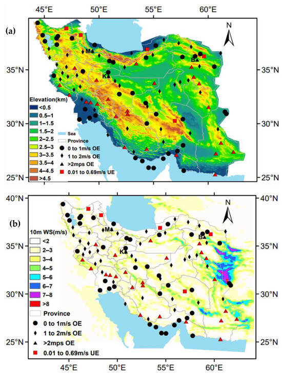
Figure 3.
(a) Topographic map of Iran and locations of the stations classified according to the various categories of BE (as in the legend) of annual 10 m wind speed; (b) various categories of BE (as in the legend) and annual mean distribution of the 10 m wind speed (shaded as in the legend) during the period 2004–2020. UE and OE stand for model underestimation and model overestimation, respectively.
The spatial distribution of the annual mean wind speed at 10 m shows that the highest wind intensities occur in the eastern part of Iran, through the Sistan Basin and in regions north of it, where the strong and persistent Levar wind blows during the warm season. This finding is consistent with the results obtained by several previous works [104,105,106,107]. All other parts of Iran present much lower wind speeds, which are generally increased along the Zagros and Alborz mountain ranges, since stronger winds occur at higher altitudes. The Iranian Plateau and coastal areas are characterized by rather weak winds, as well as the southwest part of Iran (Khuzestan Province), which is highly affected by Shamal dust storms mostly during the warm period of the year [108,109,110]. On an annual mean basis, the effect of “Qibla wind” [103] over the central Iranian Plateau seems to have a rather limited impact on the wind regime over the region.
The Global Wind Atlas (GWA) version 3 provides wind climatological data estimated on a 250 m grid at five heights (10 m, 50 m, 100 m, 150 m, and 200 m) for the period between 2008 and 2017. While the latest and most accurate available observations have been used to produce this wind dataset, in many developing countries, the lack of ground measurements from high-precision meteorological towers and LiDARs means that the data cannot be fully confirmed (https://globalwindatlas.info, accessed on 12 January 2024).
To compare the results of the WRF wind simulations with the DTU microscale wind data of the GWA, the differences between their 50 m and 100 m winds were calculated and are presented in Figure 4. The results indicate that the difference between the WRF model and the wind atlas data is small in areas with high wind speeds, showing a good agreement between the two datasets. However, in mountainous and high-altitude areas, particularly along the Zagros Mountains, the WRF model tends to overestimate the wind speeds (Figure 4e,f). Overall, it is expected that there will be differences between mesoscale wind data (grid spacing 5 km) and high-resolution wind data (grid spacing 250 m). Therefore, this comparison demonstrates that the generalized wind climate technique applied in the GWA reduced the error of DTU data in mountainous areas. However, the assessment of wind climate using the Global Wind Atlas (such as the data available in GWA website) is not as suitable because it represents the average of a long climatic period (2008–2017) and does not include measurements of wind speed throughout that entire period. Additionally, it does not provide the capability to examine the temporal distribution of wind speeds.
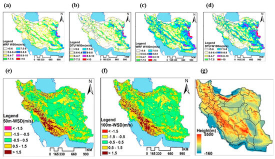
Figure 4.
Mean wind speeds (m/s) at heights of 50 m and 100 m, as generated by the WRF simulations (a,c) and the DTU wind Atlas (b,d) over Iran, along with their differences at 50 m (e) and 100 m (f). The topographic map of Iran is shown in (g).
The overestimation of wind speed in WRF simulations can be influenced by various factors, including the location and number of vertical levels, grid spacing, and the size and location of the simulation domain. According to Hahmann et al. [32], smaller domains tend to have lower wind speeds and less bias, while RMSE increases with domain size and integration time. However, analysis of these topics is beyond the scope of this study. Nonetheless, it is concluded that a suitable configuration was chosen for the simulations, and the resulting data demonstrates reasonable accuracy. This dataset can be utilized in other studies and subsequent processes to develop micro-scale wind atlases for targeted areas in the country, thus helping in wind farm development.
3.2. Mapping of the Wind Energy Potential
Overall, the total runs of the WRF model generated approximately 280 billion wind records (spatial resolution of 5 km × 5 km) over the Iranian territory, collected at levels near the Earth’s surface, specifically up to a height of 200 m above ground level. To assess the wind energy potential, monthly and seasonal averages of wind speed were analyzed at different heights, particularly at 50 m a.g.l, which is the mean height for wind turbines. The spatial distribution of wind speed over Iran at this height is shown in Figure 5, Figure 6 and Figure 7, on a monthly, seasonal and annual basis, respectively, covering the period 2004–2020.
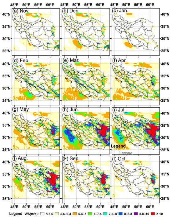
Figure 5.
Spatial distribution of the simulated monthly mean wind speeds at 50 m a.g.l. during 2004–2020 in Iran.
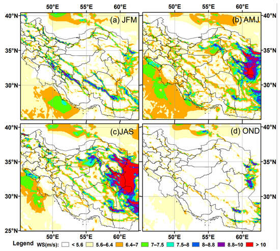
Figure 6.
Spatial distribution of the simulated seasonal mean wind speed at 50 m a.g.l. during the period 2004–2020 for (a) winter (JFM), (b) spring (AMJ), (c) summer (JJA) and (d) Autumn (OND).
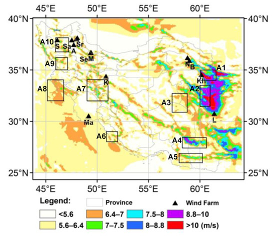
Figure 7.
Simulated mean wind speed at 50 m a.g.l. during the period 2004–2020 over Iran. The black triangles show the locations of installed wind farms: (A) Agh Kand, (B) Binaloud, (K) Kahak, (Kh) Khaf, (L) Lutak, (M) Manjil, (Ma) Mahshahr, (N) Neyshabur, (S) Sahand, (Sa) Sarab, (Se) Seyahpush, (Sr) Sareyn. The rectangles correspond to 10 areas (A1–A10), with sufficient wind potential, where long-term wind speed trends were calculated.
Based on the classification proposed by Elliott et al. [72], the wind energy potential of an area can be categorized into seven groups according to the average wind speed (AWS) at 50 m. These categories include Poor (AWS less than 5.6 m/s), Marginal (AWS of 5.6–6.4 m/s), Fair (AWS of 6.4 to 7 m/s), Good (WS of 7–7.5 m/s), Excellent (WS of 7.5–8 m/s), Outstanding (WS of 8–8.8 m/s), and Very Outstanding (above 8.8 m/s) wind energy potential. Monthly, seasonal, and annual AWS at 50 m were assessed according to this classification, as shown in Figure 5, Figure 6 and Figure 7. Figure 5 illustrates the spatial distribution of the monthly average wind speed at 50 m, starting with November, which had the lowest spatial mean wind speed. The results show that wind speeds were generally low in November, December and January, but increased from February to April in certain parts along the eastern Iranian borders, the Zagros and Alborz Mountains, and areas near the Caspian Sea and Persian Gulf. The highest wind speeds were observed from June to August, particularly in the eastern (Levar wind) and southwestern (Shamal wind) regions of the country. The strong northerly Levar flow creates an exceptional source of renewable energy and wind energy potential over the Sistan Basin and eastern regions of Iran (Figure 5g–k). By the end of the warm season, and due to changes in atmospheric circulation in central and south Asia, the wind speed gradually decreases as Levar dissipates [106].
These findings align with previous studies conducted in the eastern part of Iran, specifically in the Sistan Basin [106,111,112,113]. Consequently, the highest wind energy potential in Iran is identified along the eastern borders with Afghanistan, primarily due to the strong Levar wind that blows during the warm period of the year from May to October.
Figure 6 presents the simulations of seasonal mean 50 m wind speeds. During the winter season, only some narrow bands of high wind speeds are observed along the mountainous areas, mainly in the Zagros Mountains, while weaker winds are observed over the Persian Gulf and the central Iranian Plateau (Figure 6a). In spring, wind speeds in the mountainous areas decrease compared to winter, but they significantly increase in the eastern part of Iran with less intensity in the western and southwestern regions of the country (Figure 6b). During the summer season, the wind intensity as well as the area covered by strong winds in the eastern part of the country increase, while areas with high wind speeds in the west and southwest decrease (Figure 6c). In autumn, wind speeds are generally low throughout the country, except for some small areas with stronger winds in the eastern part (Figure 6d).
The map of the annual mean wind speed over Iran (Figure 7) reveals that the areas with the highest wind energy potential are located on top of high mountain ridges and in wind corridors, such as mountain passes. These areas, classified into class 3 (6.4–7 m/s) and above, are found in the high mountain ranges and in the Sistan Basin. However, for the mountain ranges, the wind speed and direction may be highly sensitive to atmospheric circulation and thermodynamics [114]. The wind–climatology map demonstrates that Iran has numerous regions with good or excellent wind energy potential. However, the Kavir and Lut Deserts in the interior of Iran generally have low Aeolian potential on an annual basis, with a notable seasonality. The Aeolian regime in these desert regions, along with annual and intra-seasonal variability, play a significant role in land degradation and wind erosion from the deserts and arid rangelands in central Iran [115,116,117]. Certain valleys and wind corridors along the eastern borders of Iran exhibit wind speeds of up to class 6 in terms of the annual average wind speed categorization. The channeling effect in these valleys intensifies wind intensity and modifies wind shear compared to the regional wind regime influenced by pressure gradients [105,106,107,108]. Prevailing strong winds in eastern Iran are mainly northwesterlies, aligning with the orientation of the valley corridors [111]. The Lut Valley Gap area frequently experiences strong northerly winds due to the channeling of wind flow between the topographic low belt and tall snowy mountains. These wind corridors exhibit pronounced seasonal variations in wind power density, with a peak during summer. However, other valleys and basins in the Iranian interior that lack suitable orientation in relation to the main wind flow display significantly reduced wind resources.
In Figure 7, the sites marked with black triangles represent regions where wind farms have been already established. Characteristically, the annual mean simulated wind speed in the Manjil region is approximately 7.82 m/s, in Kahak it is 6.71 m/s, and in Binaloud it is 7.11 m/s, corresponding to wind classes 5, 3 and 4, respectively. It is observed that possible wind farms in the Sistan Basin in eastern Iran would fall into the upper class 7, as the annual mean wind speed has been measured at above 8–10 m/s at the Zabol station over the long term [106,117,118]. However, despite this very outstanding wind energy potential in the Sistan Basin and surrounding areas, no wind farms or Aeolian Parks have been developed there so far. Therefore, this wind atlas for Iran highlights areas where a high level of wind resources may exist but have not been fully exploited.
In addition, ten areas with sufficient wind energy potential were detected in Figure 7 (10 rectangles), distributed over the Iranian territory except for the central Iranian Plateau. For these areas, the monthly mean wind speeds, averaged over the 17-year period (2004–2020) according to WRF simulations, are shown in Figure 8, which highlights the significantly higher wind potential in the summer months over areas like A1 and A2. In addition, the annual variability underscores the existence of two discernible wind patterns, each characterized by distinct seasonal variations. The first pattern aligns with the warm months, spanning from May to October, while the second is associated with the colder months, spanning from November to April. Throughout the colder season, minimal disparities in wind speeds are observed, with monthly mean wind speeds ranging from approximately 5.5 m/s to 7 m/s. Conversely, during the warm season, notable variations emerge, particularly in the eastern sectors of the country, where there is a markedly higher wind potential in A1 and A2. The maximum monthly averages of the wind speed in the A1 and A2 regions (12.5–14.5 m/s) in July–August (Figure 8) are similar to the measured wind speeds in Zabol, Sistan during the summer season [106,117]. The western border regions (A6 and A8), influenced by the northwesterly Shamal winds, also experience increased wind potential compared to the colder season.
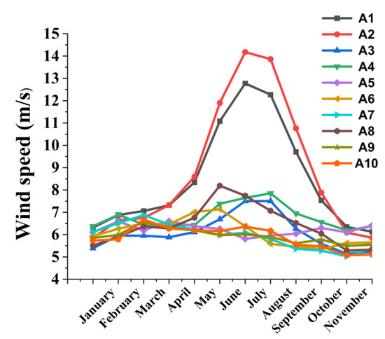
Figure 8.
The monthly mean wind speeds averaged over a 17-year period (2004–2020) based on WRF simulations for the designated regions (A1 to A10).
Furthermore, the outputs from the WRF model can be used to assess the economic feasibility of constructing wind turbine farms in appropriate areas in Iran. This evaluation involves considering the energy production capacity of wind turbines based on the simulated wind data, as well as estimating the associated costs and potential revenue from the generated electricity. Factors such as the capital investment required for constructing and maintaining wind turbines, transmission infrastructure, land availability, and government policies and incentives also need to be considered.
By combining the meteorological data from the WRF model with atmospheric pollution, financial and economic analyses [119,120,121], decision-makers can make judgments about the viability and profitability of wind energy projects in specific regions of Iran. This information can guide the selection of suitable locations for wind turbine farms, optimize the design and layout of the turbines, and support the development of policies to promote renewable energy sources. It is worth noting that while the WRF model provides valuable insights, it is essential to validate its results with ground-based measurements and consider other factors such as environmental impact assessments, social acceptance, and grid integration capabilities when making decisions regarding wind energy projects.
3.3. Trend Analysis of the Wind Energy Potential
To further investigate the trends in wind speed across the examined areas, the area’s averaged monthly and annual mean wind speeds at 50 m a.g.l were analyzed from 2004 to 2020 and the trend values are summarized in Table 9. Note that the numbers of grid points are different in each rectangle, with the biggest one being A7, with 1936 grid points, and the smallest being A9, with 572 grid points. In general, no significant trends in the wind speed were observed during the study period, indicating a rather unchanged wind energy potential across Iran. Statistically significant trends usually exceeded the slope value of ±0.06 and are highlighted with an asterisk in the table. Positive trends were detected in areas A1, A2, A4 and A5 in the eastern half of Iran during November, while some areas in eastern Iran (e.g., A1, A2, A4) showed slope values greater than 0.6 m/s in a few summer months. Furthermore, the annual trends in wind speed were insignificant in all regions except for A3 (in Lut desert), which exhibited lower wind speeds than the other regions.
Table 9.
Trend values from the linear regression of the monthly and annual wind speeds (m/s), spatially averaged over the 10 examined regions across Iran. This table also includes the number of grid points (NG) for each area. Trends equal to or greater than 0.06 (m/s) are statistically significant at the 95% confidence level and are indicated by an asterisk.
3.4. Evaluation of the WRF Simulations
To assess the accuracy of the WRF model outputs, the simulated wind speed and wind power were compared with wind observations. However, wind observations at meteorological stations were collected at a low height of 10 m a.g.l., which is not coincident with WRF simulations or suitable for wind energy assessment. Therefore, only SATBA stations that measure wind at a height of 40 m a.g.l. were used to evaluate the simulated wind-energy potential. Table 10 presents the mean, median, and wind power density (WPD) values calculated using both measured wind data and WRF simulations.
Table 10.
Comparison of the mean/median wind speed (m/s) and WPD (Wm−2) between WRF simulations and observations from SATBA wind masts at the height of 40 m.
The results show that the mean, median, and WPD values were overestimated at Hajiabad and Sheikh-Tape stations and underestimated at the other stations. The maximum errors in mean and median values were shown at Hajiabad station, with an error of 0.61 m/s and 0.94 m/s, respectively. The maximum WPD error of 158 Wm−2 was obtained at Khalkhal station. These findings suggest that while the simulated mesoscale mean wind speed provides a preliminary indication of a site’s wind energy potential, it cannot be assumed as the best estimator for wind energy production potential. Hajiabad station is an excellent example of this fact, since it presents the highest mean wind speed error but the lowest WPD error. Therefore, the mesoscale climatic wind data provide a general overview of areas with wind energy potential. However, for wind farm development, it is necessary to conduct further studies and extensive evaluations in several areas.
To further investigate this matter, Figure 9 displays the wind speed distribution for both simulated and observed data at the SATBA stations. The model slightly overestimated wind speeds above 4 m/s in Hajiabad and Sheikh-Tape stations, leading to a general overestimation of WPD in these two stations. Therefore, the model’s ability to simulate higher wind speeds has a more significant impact on WPD estimation than its overall performance. Conversely, wind speeds above 10 m/s at Koohin and Khalkhal stations and above 5 m/s at Songhor stations were underestimated by the model. On the other hand, this comparison revealed r values in the order of 0.75–0.92, indicating great consistency between the WRF-simulated and the measured wind.
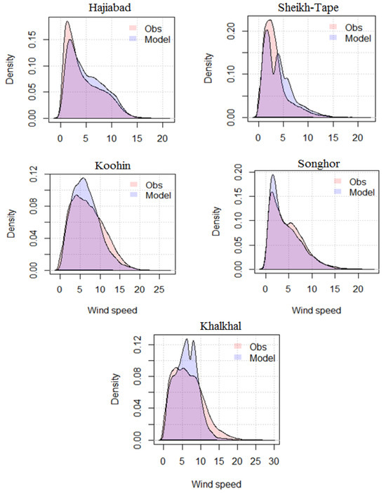
Figure 9.
Comparison of model-simulated and observed wind speed (m/s) distributions at SATBA stations.
The findings of this study demonstrate that the WRF model represents the wind speed distributions at SATBA stations in Iran with high accuracy, with some minor discrepancies observed. These results indicate that the model is reliable in assessing wind power density at selected locations in Iran and in the Middle East. However, to enhance our understanding of the Aeolian regime and wind energy potential across Iran, it is recommended to establish more SATBA stations in the future, particularly in areas affected by strong winds like the Sistan Basin. Further evaluation of the model outputs with more measured data will allow for a more comprehensive assessment of wind resources.
The current wind simulations were previously evaluated against measured wind data at ten stations around the Urmia (NW Iran) and Bakhtegan (south Iran) desiccated lakes in order to assess the influence of WRF simulations on the wind erosion and dust outbreaks from these dried lake basins [27]. The results of the simulations showed that the model overestimated 10 m wind data in all the stations around Bakhtegan Lake and it performed better at stations around Urmia Lake. The height difference (10 m vs. 50 m) may be a regulatory factor for this overestimation. The analysis also revealed RMSE values in the order of 0.5–2.4 ms−1 at the ten examined stations, with r values of 0.43 to 0.87 [27]. Furthermore, the WRF model represented the wind direction at 5 stations around the Urmia Lake fairly weel, despite some biases in the frequency and wind intensity at each direction.
The optimization and evaluation of the WRF model for wind energy resource assessment and mapping in Iran hold significant industrial relevance within the renewable energy sector [121]. The region possesses vast untapped potential for wind energy development, but accurate assessment of wind resources is a crucial step for successful project planning, financing, and operation [122,123,124]. Through the optimization of the WRF model specifically for the Iranian territory, we can improve the accuracy of wind resource assessment and provide valuable insights into the spatial distribution and variability of wind energy resources. This information is of paramount importance for scientists, developers, investors and policymakers involved in wind energy projects, enabling informed decision-making and resource optimization.
Furthermore, the current approach for mapping wind energy resources in Iran takes into account the region’s unique geographical and climatic characteristics, including complex terrain, coastal effects, and desert environments. By considering all of these factors, we empower industry stakeholders to identify optimal locations for wind farm development, considering aspects such as land availability, proximity to transmission infrastructure, and potential environmental impacts. Our research contributes to overcoming the specific challenges associated with wind energy assessment and mapping in the region, supporting the growth and sustainability of the renewable energy industry.
4. Conclusions
This study focused on simulating wind speed using the WRF model and estimated the wind energy potential in Iran covering the period 2004–2020. Through the evaluation of different PBL parameterization schemes against several ground measurements, it was found that the ACM2 scheme exhibited the best overall performance on an annual basis, while the QNSE PBL scheme performed better during the cold season. Additionally, local-closure PBL schemes during the cold season and non-local-closure PBL schemes during the warm season showed better performance, attributed to their ability to consider small/large scale eddies within the PBL.
The WRF model exhibited some biases under intense wind speed conditions, particularly in overestimating wind speeds in mountainous regions. These biases, influenced by the elevation difference between the model grid cell and the actual elevation of the station, may contribute to systematic errors in the model. However, despite these challenges, the comparison between the model’s wind simulations and observational data revealed that for over 77% of the stations, the model’s bias error was less than 2 m/s, demonstrating the WRF’s accuracy for realistic wind energy assessment studies in Iran. Furthermore, the study identified areas with high wind energy potential for the installation of wind farms and Aeolian parks, including regions along the eastern Iranian border, such as the Sistan Basin and its surroundings. The highest wind energy potential exhibited a distinct seasonality, with the maximum in summer and the minimum in late autumn, while on an annual basis, regions in eastern Iran were classified into the highest classification groups according to the average wind speeds (>7 m/s).
These results may provide practical solutions and valuable insights for industry stakeholders, facilitating informed decision making, and promoting the effective utilization of wind energy resources in the Middle East region. Furthermore, this research contributes to the transition towards renewable energy sources, aiding in the reduction in fossil fuel consumption for power and electricity generation and supporting efforts to mitigate climate change.
Supplementary Materials
The following supporting information can be downloaded at: https://www.mdpi.com/article/10.3390/app14083304/s1, Table S1: Comparison of the wind speeds simulated by the WRF model for different PBL schemes and the measured wind data at a height of 40 m in Istakah Fadashk station for July 2013 and January 2013; Figure S1: Mean diurnal patterns of wind speed from WRF simulations with different PBL schemes and wind measurements at Istakah Fadashk stations for July 2013 (a) and January 2013 (b).
Author Contributions
Conceptualization, N.H.H., A.R.S. and D.G.K.; methodology, N.H.H. and Z.G.; software, N.H.H. and A.R.S.; validation, N.H.H., M.M.P., R.-E.P.S. and A.R.S.; formal analysis, N.H.H., A.R.S. and D.G.K.; resources, N.H.H. data curation, N.H.H. and A.R.S.; writing—original draft preparation, D.G.K.; writing—review and editing, A.R.S., D.G.K., Z.G. and R.-E.P.S.; visualization, N.H.H., M.M.P., A.R.S. and N.H.H.; supervision, A.R.S., M.H. and D.G.K. All authors have read and agreed to the published version of the manuscript.
Funding
This research received no external funding.
Institutional Review Board Statement
Not applicable.
Informed Consent Statement
Not applicable.
Data Availability Statement
The datasets supporting the reported results include MODIS via Giovanni (https://giovanni.sci.gsfc.nasa.gov/giovanni/ (accessed on 12 October 2023)).
Acknowledgments
The authors acknowledge the Renewable Energy and Energy Efficiency Organization of Iran, the Iran Meteorological Organization (IRIMO) and the Atmospheric Science and Meteorology Research Center (ASMERC) for supporting and providing the essential data for this work.
Conflicts of Interest
Nasim Hossein Hamzeh is an employee of the Air and Climate Technology Company (ACTC). This paper reflects the views of the scientists and not the company. The remaining authors declare no conflicts of interest.
References
- Osobajo, O.A.; Otitoju, A.; Otitoju, M.A.; Oke, A. The Impact of Energy Consumption and Economic Growth on Carbon Dioxide Emissions. Sustainability 2020, 12, 7965. [Google Scholar] [CrossRef]
- Balint, T.; Lamperti, F.; Mandel, A.; Napoletano, M.; Roventini, A.; Sapio, A. Complexity and the economics of climate change: A survey and a look forward. Ecol. Econ. 2017, 138, 252–265. [Google Scholar] [CrossRef]
- Fouquet, R. Lessons from energy history for climate policy: Technological change, demand and economic development. Energy Res. Soc. Sci. 2016, 22, 79–93. [Google Scholar] [CrossRef]
- Yin, Z.; Liu, Z.; Liu, X.; Zheng, W.; Yin, L. Urban heat islands and their effects on thermal comfort in the US: New York and New Jersey. Ecol. Indic. 2003, 154, 110765. [Google Scholar] [CrossRef]
- Shang, K.; Xu, L.; Liu, X.; Yin, Z.; Liu, Z.; Li, X.; Yin, L.; Zheng, W. Study of Urban Heat Island Effect in Hangzhou Metropolitan Area Based on SW-TES Algorithm and Image Dichotomous Model. SAGE Open 2023, 13, 21582440231208851. [Google Scholar] [CrossRef]
- Tizpar, A.M.; Satkin, B.; Roshan, M.; Armoudli, Y. Wind Resource Assessment and Wind Power Potential of Mil-E Nader Region in Sistan and Baluchestan Province, Iran–Part 1: Annual Energy Estimation. Energy Convers. Manag. 2014, 79, 273–280. [Google Scholar] [CrossRef]
- GWEC. Global Wind Report: Annual Market Update 2017; Global Wind Energy Council: Brussels, Belgium, 2018. [Google Scholar]
- GSR, E.S.; Azees, M.; Vinodkumar, C.R.; Parthasarathy, G. Hybrid optimization enabled deep learning technique for multi-level intrusion detection. Adv. Eng. Softw. 2018, 173, 103197. [Google Scholar]
- Zhao, J.; Zhenhai, G.; Yanling, G.; Ye, Z.; Wantao, L.; Jianming, H. Wind Resource Assessment Based on Numerical Simulations and an Optimized Ensemble System. Energy Convers. Manag. 2019, 201, 112164. [Google Scholar] [CrossRef]
- SATBA. Statistics of RE Power Plants, Renewable Energy and Energy Efficiency Organization. 2019. Available online: https://www.satba.gov.ir/en/investmentpowerplants/statisticsofrepowerplants (accessed on 4 December 2023).
- Chiras, D. Power from the Wind: Achieving Energy Independence; New Society Publishers: Gabriola Island, BC, Canada, 2009. [Google Scholar]
- Carvalho, D.; Rocha, A.; Santos, C.S.; Pereira, R. Wind resource modelling in complex terrain using different mesoscale–microscale coupling techniques. Appl. Energy 2013, 108, 493–504. [Google Scholar] [CrossRef]
- Badger, J.; Frank, H.; Hahmann, A.N.; Giebel, G. Wind-climate estimation based on mesoscale and microscale modeling: Statistical-dynamical downscaling for wind energy applications. J. Appl. Meteor. Climatol. 2014, 53, 1901–1919. [Google Scholar] [CrossRef]
- Peterson, E.W.; Joseph, P.H., Jr. On the Use of Power Laws for Estimates of Wind Power Potential. J. Appl. Meteorol. 1978, 17, 390–394. [Google Scholar] [CrossRef]
- Stull, R.B. An Introduction to Boundary Layer Meteorology; Springer Science & Business Media: Berlin/Heidelberg, Germany, 2012; Volume 13. [Google Scholar]
- Zhao, Y.; Li, J.; Zhang, L.; Deng, C.; Li, Y.; Jian, B.; Huang, J. Diurnal cycles of cloud cover and its vertical distribution over the Tibetan Plateau revealed by satellite observations, reanalysis datasets, and CMIP6 outputs. Atmospheric Meas. Tech. 2023, 23, 743–769. [Google Scholar] [CrossRef]
- Siuta, D. An Analysis of the Weather Research and Forecasting Model for Wind Energy Applications in Wyoming. Ph.D. Thesis, Department of Atmospheric Science, University of Wyoming, Laramie, WY, USA, 2013. [Google Scholar]
- Do-Yong, K.; Jin-Young, K.; Jae-Jin, K. Mesoscale Simulations of Multi-Decadal Variability in the Wind Resource over Korea. Asia-Pac. J. Atmos. Sci. 2013, 49, 183–192. [Google Scholar]
- Giannaros, T.M.; Melas, D.; Ziomas, I. Performance evaluation of the Weather Research and Forecasting (WRF) model for assessing wind resource in Greece. Renew. Energy 2017, 102, 190–198. [Google Scholar] [CrossRef]
- Galvez, G.H.; Flores, R.S.; Miranda, U.M.; Martínez, O.S.; Téllez, M.C.; López, D.A.; Gómez, A.K.T. Wind resource assessment and sensitivity analysis of the levelised cost of energy. A case study in Tabasco, Mexico. Renew. Energy Focus 2019, 29, 94–106. [Google Scholar] [CrossRef]
- Jared, L.; Doubrawa, P.; Xue, L.; J Newman, A.; Draxl, C.; George Scott, G. Wind Resource Assessment for Alaska’s Offshore Regions: Validation of a 14-Year High-Resolution WRF Data Set. Energies 2019, 12, 2780. [Google Scholar] [CrossRef]
- Carvalho, D.; Rocha, A.; Gómez-Gesteira, M.; Santos, C. A sensitivity study of the WRF model in wind simulation for an area of high wind energy. Environ. Model. Softw. 2012, 33, 23–34. [Google Scholar] [CrossRef]
- Penchah, M.M.; Malakooti, H. The eastern-Iran wind-resource assessment through a planetary boundary layer simulation (2011–2015). Wind. Eng. 2019, 44, 253–265. [Google Scholar] [CrossRef]
- Hamzeh, N.H.; Ranjbar Saadat Abadi, A.; Chel Gee Ooi, M.; Habibi, M.; Schöner, W. Analyses of a Lake Dust Source in the Middle East through Models Performance. Remote Sens. 2022, 14, 2145. [Google Scholar] [CrossRef]
- Hamzeh, N.H.; Shukurov, K.; Mohammadpour, K.; Kaskaoutis, D.G.; Saadatabadi, A.R.; Shahabi, H. A comprehensive investigation of the causes of drying and increasing saline dust in the Urmia Lake, northwest Iran, via ground and satellite observations, synoptic analysis and machine learning models. Ecol. Inform. 2023, 78, 102355. [Google Scholar] [CrossRef]
- Abadi, A.R.S.; Hamzeh, N.H.; Shukurov, K.; Opp, C.; Dumka, U.C. Long-term investigation of aerosols in the Urmia Lake region in the Middle East by ground-based and satellite data in 2000–2021. Remote Sens. 2022, 14, 3827. [Google Scholar] [CrossRef]
- Hamzeh, N.H.; Abadi, A.R.S.; Kaskaoutis, D.G.; Mirzaei, E.; Shukurov, K.A.; Sotiropoulou, R.E.P.; Tagaris, E. The Importance of Wind Simulations over Dried Lake Beds for Dust Emissions in the Middle East. Atmosphere 2023, 15, 24. [Google Scholar] [CrossRef]
- Janjai, S.; Masiri, I.; Promsen, W.; Pattarapanitchai, S.; Pankaew, P.; Laksanaboonsong, J.; Bischoff-Gauss, I.; Kalthoff, N. Evaluation of wind energy potential over Thailand by using an atmospheric mesoscale model and a GIS approach. J. Wind. Eng. Ind. Aerodyn. 2014, 129, 1–10. [Google Scholar] [CrossRef]
- Nor, K.M.; Shaaban, M.; Rahman, H.A. Feasibility assessment of wind energy resources in Malaysia based on NWP models. Renew. Energy 2014, 62, 147–154. [Google Scholar] [CrossRef]
- Charabi, Y.; Al Hinai, A.; Al-Yahyai, S.; Al Awadhi, T.; Choudri, B.S. Offshore wind potential and wind atlas over the Oman Maritime Zone. Energy, Ecol. Environ. 2019, 4, 1–14. [Google Scholar] [CrossRef]
- Dörenkämper, M.; Olsen, B.T.; Witha, B.; Hahmann, A.N.; Davis, N.N.; Barcons, J.; Ezber, Y.; García-Bustamante, E.; González-Rouco, J.F.; Navarro, J.; et al. The Making of the New European Wind Atlas—Part 2: Production and evaluation. Geosci. Model Dev. 2020, 13, 5079–5102. [Google Scholar] [CrossRef]
- Hahmann, A.N.; Sīle, T.; Witha, B.; Davis, N.N.; Dörenkämper, M.; Ezber, Y.; García-Bustamante, E.; González-Rouco, J.F.; Navarro, J.; Olsen, B.T.; et al. The making of the New European Wind Atlas—Part 1: Model sensitivity. Geosci. Model Dev. 2020, 13, 5053–5078. [Google Scholar] [CrossRef]
- Ashrafi, K.; Motlagh, M.S.; Neyestani, S.E. Dust storms modeling and their impacts on air quality and radiation budget over Iran using WRF-Chem. Air Qual. Atmos. Health 2017, 10, 1059–1076. [Google Scholar] [CrossRef]
- Nabavi, S.O.; Haimberger, L.; Samimi, C. Sensitivity of WRF-chem predictions to dust source function specification in West Asia. Aeolian Res. 2017, 24, 115–131. [Google Scholar] [CrossRef]
- Foroushani, M.A.; Opp, C.; Groll, M.; Nikfal, A. Evaluation of WRF-Chem Predictions for Dust Deposition in Southwestern Iran. Atmosphere 2020, 11, 757. [Google Scholar] [CrossRef]
- Yu, E.; Bai, R.; Chen, X.; Shao, L. Impact of physical parameterizations on wind simulation with WRF V3.9.1.1 over the coastal regions of North China at PBL gray-zone resolution. Geosci. Model Dev. 2022, 15, 8111–8134. [Google Scholar] [CrossRef]
- Njuki, S.M.; Mannaerts, C.M.; Su, Z. Influence of Planetary Boundary Layer (PBL) Parameterizations in the Weather Research and Forecasting (WRF) Model on the Retrieval of Surface Meteorological Variables over the Kenyan Highlands. Atmosphere 2022, 13, 169. [Google Scholar] [CrossRef]
- Arregocés, H.A.; Rojano, R.; Restrepo, G. Sensitivity analysis of planetary boundary layer schemes using the WRF model in Northern Colombia during 2016 dry season. Dyn. Atmos. Oceans 2021, 96, 101261. [Google Scholar] [CrossRef]
- Diaz, L.R.; Santos, D.C.; Käfer, P.S.; Iglesias, M.L.; da Rocha, N.S.; da Costa, S.T.L.; Kaiser, E.A.; Rolim, S.B.A. Reanalysis profile downscaling with WRF model and sensitivity to PBL parameterization schemes over a subtropical station. J. Atmos. Sol.-Terr. Phys. 2021, 222, 105724. [Google Scholar] [CrossRef]
- Dzebre, D.E.; Adaramola, M.S. A preliminary sensitivity study of Planetary Boundary Layer parameterisation schemes in the weather research and forecasting model to surface winds in coastal Ghana. Renew. Energy 2020, 146, 66–86. [Google Scholar] [CrossRef]
- Gholami, S.; Ghader, S.; Khaleghi Zavareh, H.; Ghafarian, P. Sensitivity of the WRF model surface wind simulations to initial conditions and planetary boundary layer parameterization schemes (case study: Over Persian Gulf). Iran. J. Gheophysics 2019, 13, 14–31. [Google Scholar]
- Chadee, X.T.; Seegobin, N.R.; Clarke, R.M. Optimizing the Weather Research and Forecasting (WRF) Model for Mapping the Near-Surface Wind Resources over the Southernmost Caribbean Islands of Trinidad and Tobago. Energies 2017, 10, 931. [Google Scholar] [CrossRef]
- Berg, L.K.; Liu, Y.; Yang, B.; Qian, Y.; Olson, J.; Pekour, M.; Ma, P.-L.; Hou, Z. Sensitivity of Turbine-Height Wind Speeds to Parameters in the Planetary Boundary-Layer Parametrization Used in the Weather Research and Forecasting Model: Extension to Wintertime Conditions. Bound.-Layer Meteorol. 2019, 170, 507–518. [Google Scholar] [CrossRef]
- Balzarini, A.; Angelini, F.; Ferrero, L.; Moscatelli, M.; Pirovano, G.; Riva, G.M.; Toppetti, A.; Bolzacchini, E. Comparing WRF PBL Schemes with Experimental Data over Northern Italy. In Air Pollution Modeling and Its Application XXIII; Springer: Berlin/Heidelberg, Germany, 2014; pp. 545–549. [Google Scholar]
- Penchah, M.M.; Malakooti, H.; Satkin, M. Evaluation of planetary boundary layer simulations for wind resource study in east of Iran. Renew. Energy 2017, 111, 1–10. [Google Scholar] [CrossRef]
- Ghader, S.; Montazeri-Namin, M.; Chegini, F.; Bohluly, A. Hindcast of Surface Wind Field over the Caspian Sea Using WRF Model. In Proceedings of the 11th International Conference on Coasts, Ports and Marine Structures ICOPMAS, Tehran, Iran, 26 November 2014; pp. 24–26. [Google Scholar]
- Hamzeh, N.H.; Kaskaoutis, D.G.; Rashki, A.; Mohammadpour, K. Long-Term Variability of Dust Events in Southwestern Iran and Its Relationship with the Drought. Atmosphere 2021, 12, 1350. [Google Scholar] [CrossRef]
- Aien, M.; Mahadavi, O. On the Way of Policy Making to Reduce the Reliance of Fossil Fuels: Case Study of Iran. Sustainability 2020, 12, 10606. [Google Scholar] [CrossRef]
- Shafiei Nikabadi, M.; Ghafari Osmavandani, E.; Dastjani Farahani, K.; Hatami, A. Future Analysis to Define Guidelines for Wind Energy Production in Iran using Scenario Planning. Environ. Energy Econ. Res. 2021, 5, 1–22. [Google Scholar]
- Kalehsar, O.S. Iran's Transition to Renewable Energy: Challenges and Opportunities. Middle East Policy 2019, 26, 62–71. [Google Scholar] [CrossRef]
- Rabbani, F.; Sharifikia, M. Prediction of sand and dust storms in West Asia under climate change scenario (RCPs). Theor. Appl. Clim. 2022, 151, 553–566. [Google Scholar] [CrossRef]
- Zittis, G.; Almazroui, M.; Alpert, P.; Ciais, P.; Cramer, W.; Dahdal, Y.; Fnais, M.; Francis, D.; Hadjinicolaou, P.; Howari, F.; et al. Climate Change and Weather Extremes in the Eastern Mediterranean and Middle East. Rev. Geophys. 2022, 60, e2021RG000762. [Google Scholar] [CrossRef]
- Nourifard, S. Iran’s Transition to Wind Energy. Renew. Energy Res. Appl. 2021, 2, 179–183. [Google Scholar]
- Mohamadi, H.; Saeedi, A.; Firoozi, Z.; Zangabadi, S.S.; Veisi, S. Assessment of wind energy potential and economic evaluation of four wind turbine models for the east of Iran. Heliyon 2021, 7, e07234. [Google Scholar] [CrossRef]
- Najafi, G.; Ghobadian, B.; Tavakoli, T.; Yusaf, T. Potential of bioethanol production from agricultural wastes in Iran. Renew. Sustain. Energy Rev. 2009, 13, 1418–1427. [Google Scholar] [CrossRef]
- Najafi, G.; Ghobadian, B. LLK1694-wind energy resources and development in Iran. Renew. Sustain. Energy Rev. 2011, 15, 2719–2728. [Google Scholar] [CrossRef]
- Teimourian, A.; Bahrami, A.; Teimourian, H.; Vala, M.; Huseyniklioglu, A.O. Assessment of wind energy potential in the southeastern province of Iran. Energy Sources Part A Recover. Util. Environ. Eff. 2020, 42, 329–343. [Google Scholar] [CrossRef]
- Alavi, O.; Mohammadi, K.; Mostafaeipour, A. Evaluating the suitability of wind speed probability distribution models: A case of study of east and southeast parts of Iran. Energy Convers. Manag. 2016, 119, 101–108. [Google Scholar] [CrossRef]
- Boloorani, A.D.; Papi, R.; Soleimani, M.; Al-Hemoud, A.; Amiri, F.; Karami, L.; Samany, N.N.; Bakhtiari, M.; Mirzaei, S. Visual interpretation of satellite imagery for hotspot dust sources identification. Remote. Sens. Appl. Soc. Environ. 2023, 29, 100888. [Google Scholar] [CrossRef]
- Boroughani, M.; Pourhashemi, S.; Hashemi, H.; Salehi, M.; Amirahmadi, A.; Asadi, M.A.Z.; Berndtsson, R. Application of remote sensing techniques and machine learning algorithms in dust source detection and dust source susceptibility mapping. Ecol. Inform. 2020, 56, 101059. [Google Scholar] [CrossRef]
- Gholami, H.; Mohammadifar, A.; Pourghasemi, H.R.; Collins, A.L. A new integrated data mining model to map spatial variation in the susceptibility of land to act as a source of aeolian dust. Environ. Sci. Pollut. Res. 2020, 27, 42022–42039. [Google Scholar] [CrossRef]
- Gholami, H.; Mohamadifar, A.; Rahimi, S.; Kaskaoutis, D.G.; Collins, A.L. Predicting land susceptibility to atmospheric dust emissions in central Iran by combining integrated data mining and a regional climate model. Atmospheric Pollut. Res. 2021, 12, 172–187. [Google Scholar] [CrossRef]
- Papi, R.; Attarchi, S.; Boloorani, A.D.; Samany, N.N. Characterization of Hydrologic Sand and Dust Storm Sources in the Middle East. Sustainability 2022, 14, 15352. [Google Scholar] [CrossRef]
- Skamarock, W.C.; Klemp, J.B.; Dudhia, J.; O’Gill, D.; Barker, D.M.; Wang, W.; Powers, J.G. A Description of the Advanced Research WRF Version 3; NCAR Technical Note-475+ STR; National Center for Atmospheric Research: Boulder, CO, USA, 2008. [Google Scholar]
- Powers, J.G.; Klemp, J.B.; Skamarock, W.C.; Davis, C.A.; Dudhia, J.; Gill, D.O.; Coen, J.L.; Gochis, D.J.; Ahmadov, R.; Peckham, S.E.; et al. The Weather Research and Forecasting Model: Overview, System Efforts, and Future Directions. Bull. Am. Meteorol. Soc. 2017, 98, 1717–1737. [Google Scholar] [CrossRef]
- Louka, P.; Galanis, G.; Siebert, N.; Kariniotakis, G.; Katsafados, P.; Pytharoulis, I.; Kallos, G. Improvements in wind speed forecasts for wind power prediction purposes using Kalman filtering. J. Wind. Eng. Ind. Aerodyn. 2008, 96, 2348–2362. [Google Scholar] [CrossRef]
- Stauffer, D.R.; Seaman, N.L. Use of four-dimensional data assimilation in a limited-area mesoscale model. Part I: Experiments with synoptic-scale data. Mon. Weather. Rev. 1990, 118, 1250–1277. [Google Scholar] [CrossRef]
- Stauffer, D.R.; Seaman, N.L. Multiscale four-dimensional data assimilation. J. Appl. Meteorol. Climatol. 1994, 33, 416–434. [Google Scholar] [CrossRef]
- Spero, T.L.; Nolte, C.G.; Mallard, M.S.; Bowden, J.H. A Maieutic Exploration of Nudging Strategies for Regional Climate Applications Using the WRF Model. J. Appl. Meteorol. Clim. 2018, 57, 1883–1906. [Google Scholar] [CrossRef] [PubMed]
- Mai, X.; Qiu, X.; Yang, Y.; Ma, Y. Impacts of Spectral Nudging Parameters on Dynamical Downscaling in Summer over Mainland China. Front. Earth Sci. 2020, 8, 4754. [Google Scholar] [CrossRef]
- Mellor, G.L.; Yamada, T. A hierarchy of turbulence closure models for planetary boundary layers. J. Atmos. Sci. 1974, 31, 1791–1806. [Google Scholar] [CrossRef]
- Gryning, S.-E.; Batchvarova, E.; Floors, R. A Study on the Effect of Nudging on Long-Term Boundary Layer Profiles of Wind and Weibull Distribution Parameters in a Rural Coastal Area. J. Appl. Meteorol. Clim. 2013, 52, 1201–1207. [Google Scholar] [CrossRef][Green Version]
- Elliott, D.; Schwartz, M. Development and Validation of High-Resolution State Wind Resource Maps for the United States; NREL/TP-500-38127; National Renewable Energy Laboratory: Golden, CO, USA, 2005. [Google Scholar]
- Lin, Y.L.; Farley, R.D.; Orville, H.D. Bulk parameterization of the snow field in a cloud model. J. App. Meteo. Clim. 1983, 22, 1065–1092. [Google Scholar] [CrossRef]
- Dudhia, J. Numerical study of convection observed during the winter monsoon experiment using a mesoscale two-dimensional model. J. Atmos. Sci. 1989, 46, 3077–3107. [Google Scholar] [CrossRef]
- Niu, G.Y.; Yang, Z.L.; Mitchell, K.E.; Chen, F.; Ek, M.B.; Barlage, M.; Kumar, A.; Manning, K.; Niyogi, D.; Rosero, E.; et al. The community Noah land surface model with multiparameterization options (Noah-MP): 1. Model description and evaluation with local-scale measurements. J. Geophys. Res. Atmos. 2011, 116, 1–18. [Google Scholar]
- García-Díez, M.; Fernández, J.; Fita, L.; Yagüe, C. Seasonal dependence of WRF model biases and sensitivity to PBL schemes over Europe. Q. J. R. Meteorol. Soc. 2013, 139, 501–514. [Google Scholar] [CrossRef]
- Hong, S.-Y.; Noh, Y.; Dudhia, J. A New Vertical Diffusion Package with an Explicit Treatment of Entrainment Processes. Mon. Weather. Rev. 2006, 134, 2318–2341. [Google Scholar] [CrossRef]
- Hong, S. A new stable boundary-layer mixing scheme and its impact on the simulated East Asian summer monsoon. Q. J. R. Meteorol. Soc. 2010, 136, 1481–1496. [Google Scholar] [CrossRef]
- Abdella, K.; McFarlane, N. A new second-order turbulence closure scheme for the planetary boundary layer. J. Atmos. Sci. 1997, 54, 1850–1867. [Google Scholar] [CrossRef]
- Janjić, Z.I. The Step-Mountain Eta Coordinate Model: Further Developments of the Convection, Viscous Sublayer, and Turbulence Closure Schemes. Mon. Weather. Rev. 1994, 122, 927–945. [Google Scholar] [CrossRef]
- Nakanishi, M.; Hiroshi, N. An Improved Mellor–Yamada Level-3 Model: Its Numerical Stability and Application to a Regional Prediction of Advection Fog. Bound.-Layer Meteorol. 2006, 119, 397–407. [Google Scholar] [CrossRef]
- Sukoriansky, S.; Galperin, B.; Perov, V. Application of a New Spectral Theory of Stably Stratified Turbulence to the Atmospheric Boundary Layer over Sea Ice. Bound -Layer Meteorol. 2005, 117, 231–257. [Google Scholar] [CrossRef]
- Pleim, J.E. A Combined Local and Nonlocal Closure Model for the Atmospheric Boundary Layer. Part I: Model Description and Testing. J. Appl. Meteorol. Climatol. 2007, 46, 1383–1395. [Google Scholar] [CrossRef]
- Mostafaeipour, A.; Jadidi, M.; Mohammadi, K.; Sedaghat, A. An analysis of wind energy potential and economic evaluation in Zahedan, Iran. Renew. Sustain. Energy Rev. 2014, 30, 641–650. [Google Scholar] [CrossRef]
- Conradsen, K.; Nielsen, L.B.; Prahm, L.P. Review of Weibull Statistics for Estimation of Wind Speed Distributions. J. Clim. Appl. Meteorol. 1984, 23, 1173–1183. [Google Scholar] [CrossRef]
- Chandel, S.; Ramasamy, P.; Murthy, K. Wind power potential assessment of 12 locations in western Himalayan region of India. Renew. Sustain. Energy Rev. 2014, 39, 530–545. [Google Scholar] [CrossRef]
- Solyali, D.; Altunç, M.; Tolun, S.; Aslan, Z. Wind resource assessment of Northern Cyprus. Renew. Sustain. Energy Rev. 2016, 55, 180–187. [Google Scholar] [CrossRef]
- Carvalho, D.; Rocha, A.; Gómez-Gesteira, M.; Santos, C.S. Sensitivity of the WRF model wind simulation and wind energy production estimates to planetary boundary layer parameterizations for onshore and offshore areas in the Iberian Peninsula. Appl. Energy 2014, 135, 234–246. [Google Scholar] [CrossRef]
- Stensrud, D.J. Parameterization Schemes: Keys to Understanding Numerical Weather Prediction Models; Cambridge University Press: Cambridge, UK, 2009. [Google Scholar]
- Shin, H.H.; Hong, S.Y. Intercomparison of Planetary Boundary-Layer Parametrizations in the WRF Model for a Single Day from CASES-99. Bound. -Layer Meteorol. 2011, 139, 261–281. [Google Scholar] [CrossRef]
- Stull, R.B. Transilient Turbulence Theory. Part I: The Concept of Eddy-Mixing across Finite Distances. J. Atmos. Sci. 1984, 41, 3351–3367. [Google Scholar] [CrossRef]
- Troen, I.B.; Mahrt, L. A simple model of the atmospheric boundary layer; sensitivity to surface evaporation. Bound.-Layer Meteorol. 1986, 37, 129–148. [Google Scholar] [CrossRef]
- Bright, D.R.; Mullen, S.L. The Sensitivity of the Numerical Simulation of the Southwest Monsoon Boundary Layer to the Choice of PBL Turbulence Parameterization in MM5. Weather. Forecast. 2002, 17, 99–114. [Google Scholar] [CrossRef]
- Misenis, C.; Yang, Z. An Examination of Sensitivity of WRF/Chem Predictions to Physical Parameterizations, Horizontal Grid Spacing, and Nesting Options. Atmos. Res. 2010, 97, 315–334. [Google Scholar] [CrossRef]
- Deng, A.; David, R.S. On Improving 4-Km Mesoscale Model Simulations. J. Appl. Meteorol. Climatol. 2006, 45, 361–381. [Google Scholar] [CrossRef]
- Zhao, H.; Che, H.; Xia, X.; Wang, Y.; Wang, H.; Wang, P.; Ma, Y.; Yang, H.; Liu, Y.; Wang, Y.; et al. Climatology of mixing layer height in China based on multi-year meteorological data from 2000 to 2013. Atmos. Environ. 2019, 213, 90–103. [Google Scholar] [CrossRef]
- Saha, S.; Sharma, S.; Chhabra, A.; Kumar, K.N.; Kumar, P.; Kamat, D.; Lal, S. Impact of dust storm on the atmospheric boundary layer: A case study from western India. Nat. Hazards 2022, 113, 143–155. [Google Scholar] [CrossRef]
- Basart, S.; Vendrell, L.; Baldasano, J.M. High-resolution dust modelling over complex terrains in West Asia. Aeolian Res. 2016, 23, 37–50. [Google Scholar] [CrossRef]
- Xie, X.; Xie, B.; Cheng, J.; Chu, Q.; Dooling, T. A simple Monte Carlo method for estimating the chance of a cyclone impact. Nat. Hazards 2021, 107, 2573–2582. [Google Scholar] [CrossRef]
- Solomos, S.; Abuelgasim, A.; Spyrou, C.; Binietoglou, I.; Nickovic, S. Development of a dynamic dust source map for NMME-DREAM v1.0 model based on MODIS Normalized Difference Vegetation Index (NDVI) over the Arabian Peninsula. Geosci. Model Dev. 2019, 12, 979–988. [Google Scholar] [CrossRef]
- Kontos, S.; Liora, N.; Giannaros, C.; Kakosimos, K.; Poupkou, A.; Melas, D. Modeling natural dust emissions in the central Middle East: Parameterizations and sensitivity. Atmos. Environ. 2018, 190, 294–307. [Google Scholar] [CrossRef]
- Prakash, P.J.; Stenchikov, G.; Kalenderski, S.; Osipov, S.; Bangalath, H. The impact of dust storms on the Arabian Peninsula and the Red Sea. Atmos. Meas. Tech. 2015, 15, 199–222. [Google Scholar] [CrossRef]
- Mohammadpour, K.; Sciortino, M.; Kaskaoutis, D.G. Classification of weather clusters over the Middle East associated with high atmospheric dust-AODs in West Iran. Atmospheric Res. 2021, 259, 105682. [Google Scholar] [CrossRef]
- Choobari, O.A.; Zawar-Reza, P.; Sturman, A. Low level jet intensification by mineral dust aerosols. Ann. Geophys. 2013, 31, 625–632. [Google Scholar] [CrossRef]
- Kaskaoutis, D.G.; Rashki, A.; Houssos, E.E.; Mofidi, A.; Goto, D.; Bartzokas, A.; Francois, P.; Legrand, M. Meteorological aspects associated with dust storms in the Sistan region, southeastern Iran. Clim. Dyn. 2015, 45, 407–424. [Google Scholar] [CrossRef]
- Karami, S.; Hamzeh, N.H.; Noori, F.; Ranjbar, A. Investigation of dust storms in Ilam and the performance analysis of simulation of 6 numerical prediction models at a severe dust storm in west of Iran. J. Air Pollut. Health 2019, 4, 16–32. [Google Scholar] [CrossRef]
- Francis, D.B.K.; Flamant, C.; Chaboureau, J.-P.; Banks, J.; Cuesta, J.; Brindley, H.; Oolman, L. Dust emission and transport over Iraq associated with the summer Shamal winds. Aeolian Res. 2017, 24, 15–31. [Google Scholar] [CrossRef]
- Hamzeh, N.H.; Karami, S.; Kaskaoutis, D.G.; Tegen, I.; Moradi, M.; Opp, C. Atmospheric Dynamics and Numerical Simulations of Six Frontal Dust Storms in the Middle East Region. Atmosphere 2021, 12, 125. [Google Scholar] [CrossRef]
- Abadi, A.R.S.; Hamzeh, N.H.; Ooi, M.C.G.; Kong, S.S.-K.; Opp, C. Investigation of Two Severe Shamal Dust Storms and the Highest Dust Frequencies in the South and Southwest of Iran. Atmosphere 2022, 13, 1990. [Google Scholar] [CrossRef]
- Karami, S.; Hamzeh, N.H.; Abadi, A.R.S.; Madhavan, B.L. Investigation of a severe frontal dust storm over the Persian Gulf in February 2020 by CAMS model. Arab. J. Geosci. 2021, 14, 1–12. [Google Scholar] [CrossRef]
- Rashki, A.; Middleton, N.; Goudie, A. Dust storms in Iran—Distribution, causes, frequencies and impacts. Aeolian Res. 2021, 48, 100655. [Google Scholar] [CrossRef]
- Abbasi, H.; Opp, C.; Groll, M.; Rohipour, H.; Gohardoust, A. Assessment of the distribution and activity of dunes in Iran based on mobility indices and ground data. Aeolian Res. 2019, 41, 100539. [Google Scholar] [CrossRef]
- Gholami, H.; Mohamadifar, A.; Sorooshian, A.; Jansen, J.D. Machine-learning algorithms for predicting land susceptibility to dust emissions: The case of the Jazmurian Basin, Iran. Atmos. Pollut. Res. 2020, 11, 1303–1315. [Google Scholar] [CrossRef]
- Lu, S.; Zhu, G.; Meng, G.; Lin, X.; Liu, Y.; Qiu, D.; Xu, Y.; Wang, Q.; Chen, L.; Li, R.; et al. Influence of atmospheric circulation on the stable isotope of precipitation in the monsoon margin region. Atmos. Res. 2024, 298, 107131. [Google Scholar] [CrossRef]
- Behrooz, R.D.; Mohammadpour, K.; Broomandi, P.; Kosmopoulos, P.G.; Gholami, H.; Kaskaoutis, D.G. Long-term (2012–2020) PM10 concentrations and increasing trends in the Sistan Basin: The role of Levar wind and synoptic meteorology. Atmos. Pollut. Res. 2022, 13, 101460. [Google Scholar] [CrossRef]
- Dai, S.; Chen, X.; Liang, J.; Li, X.; Li, S.; Chen, G.; Chen, Z.; Bin, J.; Tang, Y.; Li, X. Response of PM2.5 pollution to meteorological and anthropogenic emissions changes during COVID-19 lockdown in Hunan Province based on WRF-Chem model. Environ. Pollut. 2023, 331, 121886. [Google Scholar] [CrossRef] [PubMed]
- Cuevas-Figueroa, G.; Stansby, P.K.; Stallard, T. Accuracy of WRF for prediction of operational wind farm data and assessment of influence of upwind farms on power production. Energy 2022, 254, 124362. [Google Scholar] [CrossRef]
- Hamidianpour, M.; Jahanshahi, S.M.A.; Kaskaoutis, D.G.; Rashki, A.; Nastos, P.G. Climatology of the Sistan Levar wind: Atmospheric dynamics driving its onset, duration and withdrawal. Atmos. Res. 2021, 260, 105711. [Google Scholar] [CrossRef]
- Prósper, M.A.; Otero-Casal, C.; Fernández, F.C.; Miguez-Macho, G. Wind power forecasting for a real onshore wind farm on complex terrain using WRF high resolution simulations. Renew. Energy 2019, 135, 674–686. [Google Scholar] [CrossRef]
- Chen, X.; Li, X.; Liang, J.; Li, X.; Li, S.; Chen, G.; Chen, Z.; Dai, S.; Bin, J.; Tang, Y. Causes of the unexpected slowness in reducing winter PM2.5 for 2014–2018 in Henan Province. Environ. Pollut. 2023, 319, 120928. [Google Scholar] [CrossRef]
- Abdi, A.; Astaraei, F.R.; Rajabi, N. GIS-AHP-GAMS based analysis of wind and solar energy integration for addressing energy shortage in industries: A case study. Renew. Energy 2024, 225, 120295. [Google Scholar] [CrossRef]
- Zahedi, R.; Sadeghitabar, E.; Khazaee, M.; Faryadras, R.; Ahmadi, A. Potentiometry of wind, solar and geothermal energy resources and their future perspectives in Iran. Environ. Dev. Sustain. 2024, 1–27. [Google Scholar] [CrossRef]
- Abdolahinia, H.; Heidarizadeh, M.; Rahmati, I. Assessing Iran and its neighbors for prospects and challenges: The case of the electrical sector. Renew. Sustain. Energy Rev. 2024, 193, 114190. [Google Scholar] [CrossRef]


Disclaimer/Publisher’s Note: The statements, opinions and data contained in all publications are solely those of the individual author(s) and contributor(s) and not of MDPI and/or the editor(s). MDPI and/or the editor(s) disclaim responsibility for any injury to people or property resulting from any ideas, methods, instructions or products referred to in the content. |
© 2024 by the authors. Licensee MDPI, Basel, Switzerland. This article is an open access article distributed under the terms and conditions of the Creative Commons Attribution (CC BY) license (https://creativecommons.org/licenses/by/4.0/).