
Numerical Study of a Latent Heat Storage System’s Performance as a Function of the Phase Change Material’s Thermal Conductivity


Mechanical Engineering, Dalhousie University, Halifax, NS B3H 4R2, Canada
*
Author to whom correspondence should be addressed.
Appl. Sci. 2024, 14(8), 3318; https://doi.org/10.3390/app14083318
Submission received: 25 March 2024
/
Revised: 9 April 2024
/
Accepted: 12 April 2024
/
Published: 15 April 2024
(This article belongs to the Special Issue Advances in Materials for Thermal Energy Storage)
Abstract
:Featured Application
Guidance in the development of phase change materials (PCMs), as well as knowledge towards the design and development of latent heat thermal energy storage (LHTES) systems.
Abstract
The thermal conductivities of most commonly used phase change materials (PCMs) are typically fairly low (in the range of 0.2 to 0.4 W/m·K) and are an important consideration when designing latent heat energy storage systems (LHESSs). Because of that, material scientists have been asking the following question: “by how much does the thermal conductivity of a PCM needs to be increased to positively impact the design and performance of a LHESS?” The answer to this question is not straightforward as the performance of a LHESS depends on the PCM’s thermal conductivity, other PCM thermophysical properties, the type of heat exchange system geometry used, the mode of operation, and the targeted power/energy storage of the LHESS. This paper presents work related to this question through a numerical study based on a simplified 2D model of an experimental setup studied previously in the authors’ laboratory. A model created in COMSOL Multiphysics, based on conduction and accounting for the solid-liquid phase change process, was initially validated against experimental results and then used to study the impact of the PCM’s thermal conductivity (dodecanoic acid) on the discharging power of the LHESS. The results show that even increasing the thermal conductivity of the PCM by a factor of 50 only leads to a maximum instantaneous power increase by a factor of 2 or 3 depending on the LHESS configurations.
1. Introduction
With the ever-increasing emergence of renewable energy technologies in the overall worldwide energy production [1], it is now clear that energy storage solutions are needed to deal with natural fluctuations in the availability of renewables [2]. Knowing that a large percentage of energy end-use is in the form of thermal energy (space heating and cooling, domestic hot water, power generation, thermally driven industrial processes, etc.), it appears logical that energy could be stored thermally in these instances, especially when it has been demonstrated that thermal energy storage (TES) is a less expensive option compared to electrical storage [3]. For example, storing heat in water (or other sensible storage media like rocks) is very inexpensive compared to electrical storage in Li-ion batteries. In contrast, it is very clear that the quality of energy stored in a Li-ion battery is much greater than that stored in a given mass of water (try charging your smartphone from a hot water tank).
That is to say that TES solutions still face many challenges, of which the main one is designing a system that matches the need of a given application at a competitive market price [4]. Latent heat energy storage systems (LHESSs) use phase change materials (PCMs) to store heat with a much greater energy density than sensible heat, through their solid-liquid phase transition [5]. LHESSs also offer the advantage that the phase transition of the PCM happens over a small and well-defined temperature range, allowing for more efficient design of components linked to the LHESS [6,7].
Both the selection of thermophysical properties of the PCM [8,9] and the design of the heat exchange system [4,10,11,12] are central parts in the design of a LHESS. The solid-liquid phase transition temperature often plays the most important role in the selection of a specific PCM for a given application, depending on the operating temperature range of that application. The latent heat and, to a certain extent, specific heat of a PCM are central to its ability to store thermal energy [13].
However, for the design of a LHESS based on transient operation, the (typically) very small thermal conductivity of PCMs (apart from metallic ones and exceptions [14]) are in the order of 0.2 to 0.4 W/m·K [15], leading to limitations on how rapidly heat can be transferred in and out of the storage system, i.e., the “rate problem” [16]. The rate problem is currently more often addressed by designing the heat exchange system used in a LHESS to increase the heat transfer rate to a desired value, for example through the use of additional heat transfer fluid (HTF) passes [5,17], the addition of fins [18,19,20], increasing the contact area [21,22,23], or by favoring close-contact melting during the charging phase [24,25,26]. These approaches aim to optimize the efficiency and performance of LHESSs by overcoming limitations posed by the PCM’s thermal conductivity.
Increasing the PCM’s thermal conductivity could also directly affect that material’s ability to move heat to and from the exchange media, increasing the system’s heat transfer rate [27]. But by how much does the thermal conductivity of a PCM need to be increased to positively impact the design and performance of a LHESS? This question was asked by material scientists from the International Energy Agency (IEA) Annex 40/Annex 67 expert group on Compact Thermal Energy Storage. Optimizing PCM thermal conductivity holds the potential for cost benefits, offering a cheaper solution compared to relying on modifications to heat exchange systems.
This increase in thermal conductivity has been attempted through the addition of conductive nanoparticles [28,29,30]. Numerous issues are impeding the widespread use of those nano-enhanced PCMs (NePCMs), including thermal limitations still stemming from the minimal thermal conductivity increase [31], the cyclability of those systems, the economics of higher NePCM costs, etc. [28]. These same material scientists have tools in their arsenal to design new PCMs with higher thermal conductivities. However, determining the optimal increase in thermal conductivity remains a complex challenge due to the interplay of numerous parameters and properties affecting PCM behavior throughout cyclic operation.
This is a very complex question to answer since the melting and solidification of a PCM during the cyclic operation of a LHESS depend on numerous interrelated parameters and properties, with the importance of the thermal conductivity of the PCM varying throughout the process and for different geometries and operating parameters. The work presented in this paper, therefore, aims at answering this question for a given LHESS that was studied and characterized experimentally in the author’s Laboratory of Applied Multiphase Thermal Engineering (LAMTE) at Dalhousie University [18]. A simplified numerical model, accounting for conductive heat transfer in the PCM as well as the solid-liquid phase change process, was validated using experimentally measured heat transfer rates during the discharging of the system. From this validated model, a numerical parametric study was performed to determine the system’s behavior, in terms of overall heat transfer rates, for increasing thermal conductivity values of a hypothetical PCM, having all the same other thermophysical properties as the PCM used (dodecanoic acid) in the experimental work.
2. Physical Model
2.1. Experimental Setup and Geometry
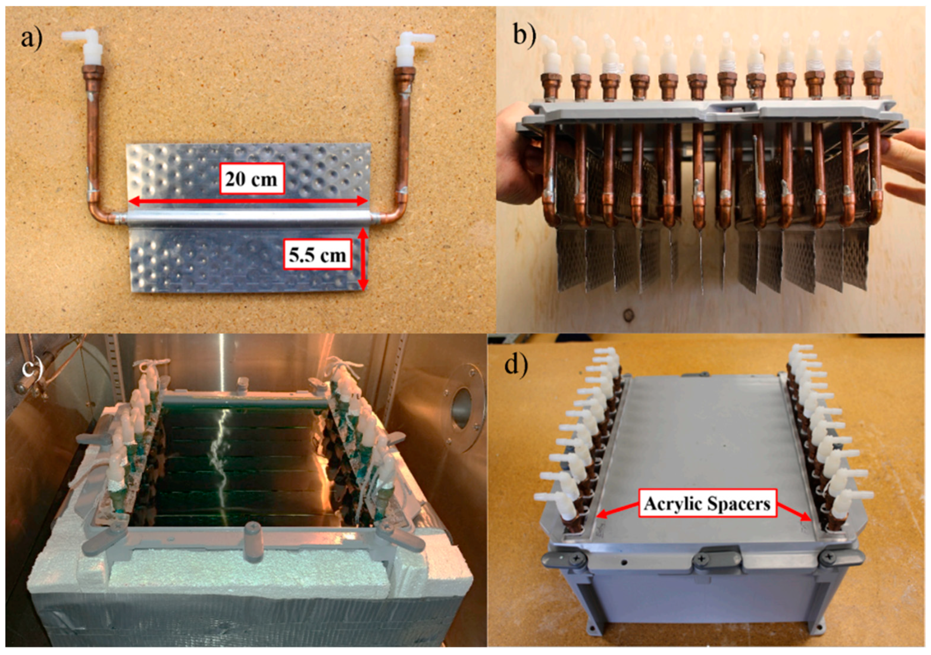
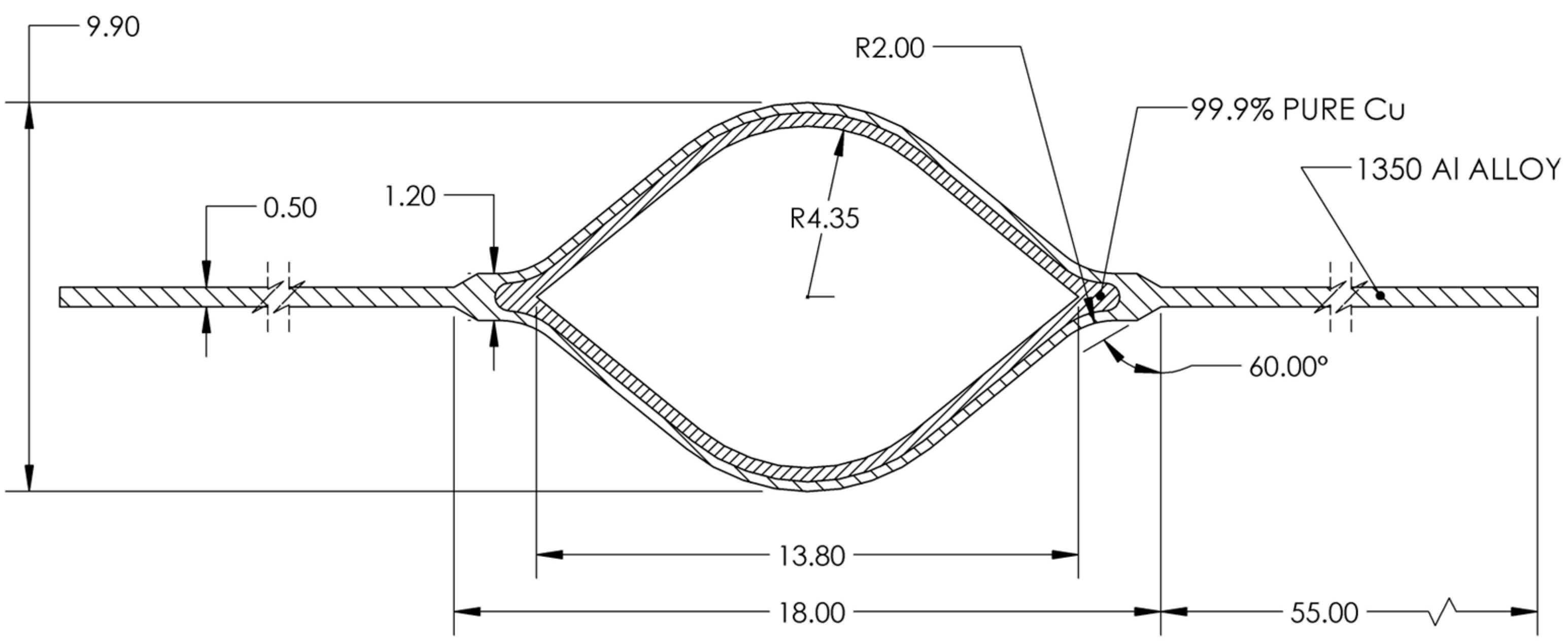
The experimental apparatus, used in Herbinger and Groulx [18], was made with multiples of the same aluminum finned-tube geometry, as seen in Figure 1a,b. Once assembled, the finned-tube heat exchanger was incorporated in a box containing 10 kg of PCM and measuring 30 cm × 30 cm × 15.25 cm (Figure 1c,d). The fin dimensions are shown in Figure 2.
The experimental apparatus was arranged in 4, 8, and 12 (evenly spaced) fin configurations which were tested at HTF flowrates (water) of 6, 9, and 12 LPM. The charging and discharging of the LHESS were tested at initial and final temperatures varying from 21 to 65 °C. At the start of each experiment, the inlet HTF temperature was ramped up or down from the initial PCM temperature to the desired final PCM temperature, and the system was left to fully charge or discharge to steady state from that point.
2.2. Material Properties
The PCM used in this study was dodecanoic acid, for which all the required thermophysical data are presented in Table 1. The materials making up the fin were pure copper and 1350 aluminum alloy, with these having defined material profiles in COMSOL Multiphysics.
3. Numerical Model
3.1. Geometry
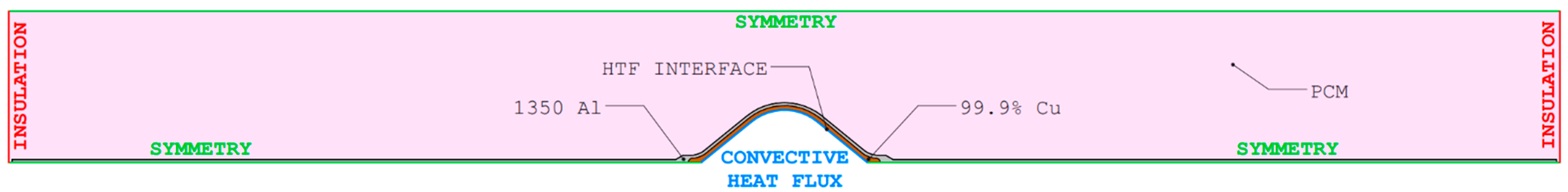
For the purpose of this numerical study, a 2D sub-domain representing half of a finned tube (and half of the distance between two finned tubes) was modelled in SolidWorks, as shown in Figure 3. The 2D geometry was then imported into COMSOL Multiphysics 6.0 for simulation with appropriate symmetry and insulated boundary conditions.
For the simulation to be representative of the experimental setup and experimental results, particularly in terms of the total mass of PCM in the system, it was assumed that the domain would be 30 cm deep (in the third dimension into the page), while the PCM domain was calculated to be 12.8525 cm high when having a fin spacing of 2.5 cm for 12 fins in the system for the system containing 10 kg of PCM.
Specific to the finned-tube geometry, shown in Figure 2, the thickness of the thin extending aluminum fin was 0.5 mm. Overall, the fin length and PCM depth were kept constant, while the fin spacing was varied to keep the mass of PCM constant in the model. This required calculations to slightly adjust the fin spacing, changing from the theoretical 2.5 cm, 3.75 cm, and 7.5 cm to 2.5 cm, 3.691 cm, and 7.263 cm for 12, 8, and 4 fins, respectively. This change yielded a negligible change in the behavior of the system when compared.
Therefore, the geometry used is shown with the boundary definitions in Figure 3. In the COMSOL model, the entire rectangular domain is meant to be rotated 90 degrees clockwise so that the insulation boundaries (red) are on the top and the bottom; it is presented in this orientation in this paper for space constraints. The symmetry line of the fin and the edge of the PCM domain are defined with a symmetry condition (green), reducing the simulation domain size, and hence the simulation time and file size. The HTF surface (blue) is defined through a convective heat flux using Newton’s law of cooling. The convection coefficient is determined through empirical correlations detailed in Section 3.4, and the HTF temperature is a function of time coming from the experimental inlet temperature data that were ramped up or down at the start of experimental runs, as mentioned previously.
3.2. Heat Transfer Physics
As demonstrated experimentally [33], conduction is the dominant mode of heat transfer during the solidification of PCM (natural convection is present in the cooling liquid PCM during this process but can mostly be neglected [34]). Therefore, COMSOL Multiphysics 6.0 was used to perform the numerical modelling using the heat transfer in solids module to solve the transient conduction equation with temperature (and time) as dependent properties; this equation is pre-defined within the classical transient heat conduction module in COMSOL Multiphysics.
The heat transfer rate from the solidifying PCM to the HTF for the half-fin geometry modelled was calculated using COMSOL’s built in Line Integration function with the expression ht.ntflux, which finds the normal total heat flux crossing the fin surface at every time step (in units of W/m). This heat transfer rate was then multiplied by 2 to obtain the power per fin, then multiplied by the system’s number of fins and the system depth (30 cm) to find the system equivalent power (in W) presented as results in the rest of this paper.
3.3. Energy Conservation and Phase Change Modelling
Energy conservation has been successfully modelled with COMSOL Multiphysics in previous studies by modifying the specific heat capacity of the PCM to simulate the latent heat of fusion () for phase change once the melting temperature () is reached [35,36]. The phase change effect is based around a piecewise melt fraction function:
where this piecewise function models the state of the PCM as a solid with a value of 0 and liquid with a value of 1 and varies linearly between 0 and 1 over the mushy zone, defined over an interval ΔT around the melting temperature Tm. This function was used to define the change in PCM properties from solid to liquid as can be seen in Equation (3). The latent heat of fusion component of the modified specific heat capacity was created by applying a Gaussian function centered about [37].
The Gaussian function has a value of zero except within the interval of Tm − ΔT/2 to Tm + ΔT/2. The function integrated over the range of all temperatures is equal to 1, which allows D(T) to be multiplied by L to produce an energy balance through the phase change, centered about Tm. Using D(T) combined with the melt fraction function ϕ(T) creates the modified specific heat capacity function:
A similar function (excluding the latent heat of fusion) was created for the thermal conductivity to simulate the gradual change in k as the PCM transitions between the solid and liquid phase in the mushy zone:
The density of the PCM was considered constant in the simulation to ensure the conservation of mass and energy, since the volume changes of the PCM were not simulated. The selected density value was the average between the solid and liquid density values: = 907.5 kg/m3.
3.4. Convective Boundary Modelling
In order to more accurately simulate the overall thermal and phase change processes within the PCM, it was imperative to capture as closely as possible the order of magnitude of the convection coefficient related to the HTF on the inside surface of the finned tube. For the various experimental trials used as the basis for this numerical study, the internal flow in the tube was in the transition region, with Reynolds numbers varying from 1000 to 4600, based mainly on flow rates and the number of finned tubes in the parallel configuration and calculated at the final HTF temperature. Therefore, using correlations from Chapter 5 of Rohsenow, et al. [38] defined for 2100 ≤ Re ≤ 106 and the assumption of uniform wall temperature:
with and . The required friction factor () for this Nusselt number correlation is defined as:
Considering the effect of entrance length on the convection coefficient, it was determined that a weighted average approach was the most physically meaningful and accurate. Equation (7) presents the entrance length correction to be applied to Nut (=Nu∞) determined from Equation (5). The constants C and n were selected for the 90° round bend case presented in Rohsenow, et al. [38].
Finally, since this entrance region correction is dependent on the distance from the 90° bend, a weighted average () was taken. Local corrected Num values were calculated at every centimeter over the 30 cm length of the finned tube, integrated over the last 29 cm using Riemann’s sums, then divided by 29 slices. The average convection coefficient used in a given simulation was calculated from the standard definition of the Nusselt number.
As mentioned earlier, values of Re for the experimental trials varied from 1000 to 4600, with the correlation in Equation (5) being valid for Re ≥ 2100. It is important to mention that convection coefficients coming from Equation (5) were found to be more accurate and therefore led to simulation results matching experimental validation data better than the purely laminar correlation from Re < 2100. Therefore, the correlation of Equation (5) was used for all numerical studies. The calculated convection coefficients for each validated experiment will be presented in Section 3.7.
3.5. Mesh Independence Study
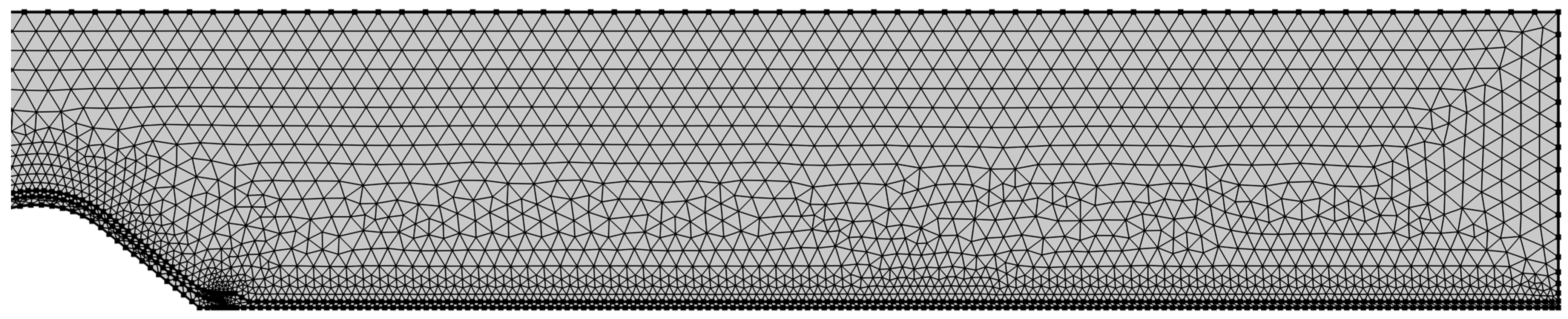
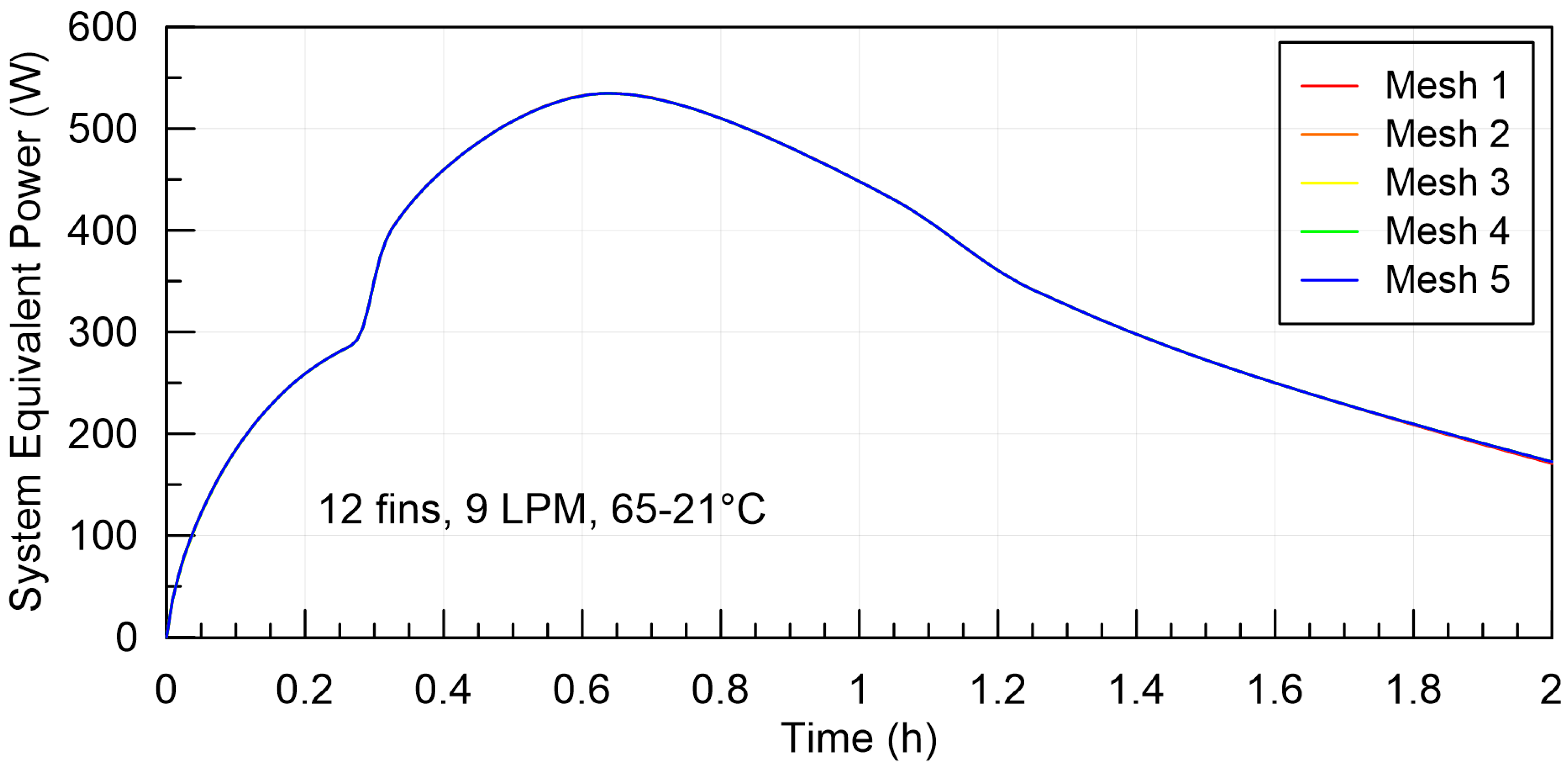
A mesh independence study was performed to determine the effect of mesh quality on numerical results. Only free-triangular elements were used to create the mesh for these numerical simulations, as shown in Figure 4. The meshing size steps were set differently for the fin and the PCM domains, with the fin being much smaller and not experiencing phase change. Five mesh sizes were used to study the effect of varying the average element sizes in both the fin and PCM domains, as shown in Table 2.
Every mesh study simulation had a time step of 30 s and simulation time of 7200 s, using the model with 12 finned tubes, a flow rate of 9 LPM, a discharging temperature range of 65 to 21 °C, and a mushy-zone temperature range of ΔT = 4 K. A defined temperature on the inner side of the copper HTF interface was used at this stage instead of a convective boundary condition and was ramped down using the function made from the experimental data as mentioned previously.
Figure 5 shows the system’s equivalent power; the difference in the studied mesh made a negligible difference. Though negligible, a mesh was selected, as outlined in, Section 3.6 following the mushy-zone range study.
3.6. Impact of Mushy-Zone Temperature Range
The mushy-zone temperature range (ΔT) defines how rapidly the PCM properties change from the liquid to solid values as a function of temperature, and over which range of temperature latent heat is accounted for during the phase change. As presented by C. Kheirabadi and Groulx [37], the mushy-zone temperature range (ΔT) also has an impact on the simulated results when the solid–liquid phase change is accounted for. Previous studies have also shown that the smallest ΔT values lead to more physically accurate results at the expense of increased computational cost [36]. Therefore, simulations were performed to look at the impact of ΔT on the local results and on the extracted power results.
The effect of modifying ΔT was studied regarding its impact on the conductive heat transfer and phase change behavior through a parametric mushy-zone ΔT study. The simulations used mesh 3, as defined in Section 3.5, and were otherwise identical to the simulations ran in Section 3.5 for the mesh independence study.
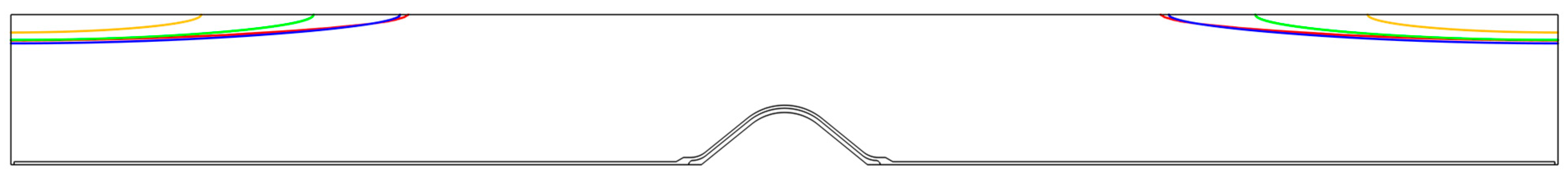
Figure 6 presents the position of the solidification interface after 7020 s for the four values of ΔT used (1, 4, 8, and 12 K). The results are shown at such a long time after the start of solidification because the impact of the mushy-zone temperature range (ΔT) becomes more noticeable then. It can be observed that the position of the interface, therefore the amount of PCM solidified, varies slightly with values of ΔT. The position of the interface is mostly the same for ΔT of 1 and 4 K, with the difference increasing with an increase in ΔT.
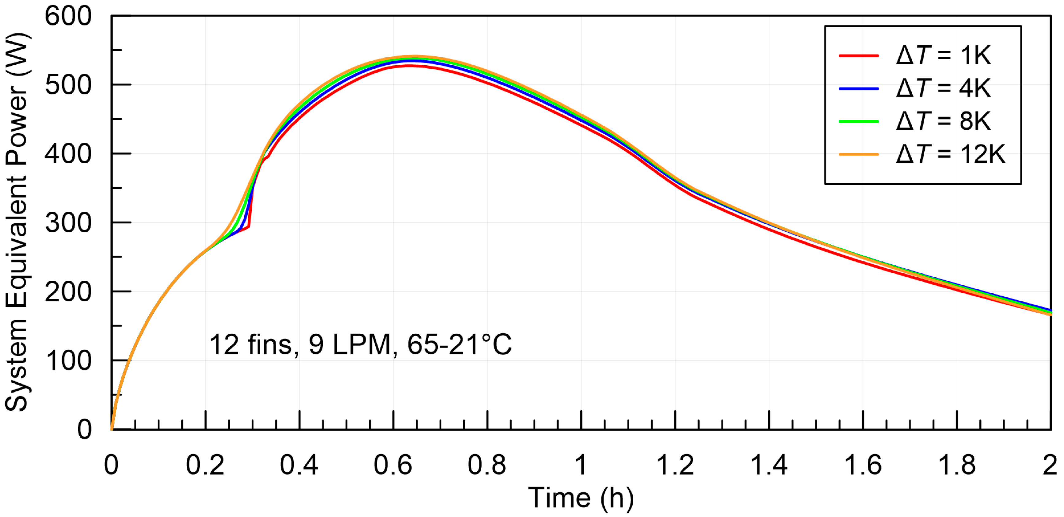
Figure 7 shows the effect of changing ΔT on the system equivalent power curve. In reality, there is no mushy range for the PCM used. Rather, the material goes through its phase transition at a well-defined melting/solidification temperature, and the impact of the latent heat of fusion is felt solely at this transition temperature. Therefore, numerically, increasing ΔT yields a smoother, more continuous power curve with a slightly higher value for the system equivalent power. When ΔT = 1 K, the power curve closer mimics the discontinuous behavior seen in the experimental data at approximately 1250 s.
Also, as ΔT decreases, the modified specific heat capacity function becomes much steeper and taller due to the latent heat correction having to be accounted for within a smaller temperature range. Numerically, this makes the simulation more time consuming and causes convergence issues when varying thermal conductivities individually. Therefore, a ΔT = 2 K was chosen to perform the simulations for this study.
Finally, for the final mesh selection, mesh 3 (from Table 2) was selected, composed of approximately 16,000 elements (for 12 finned tubes). This mesh also eliminated some convergence issues encountered when using coarser meshes with the selected mushy-zone temperature range of ΔT = 2 K.
3.7. Model Validation
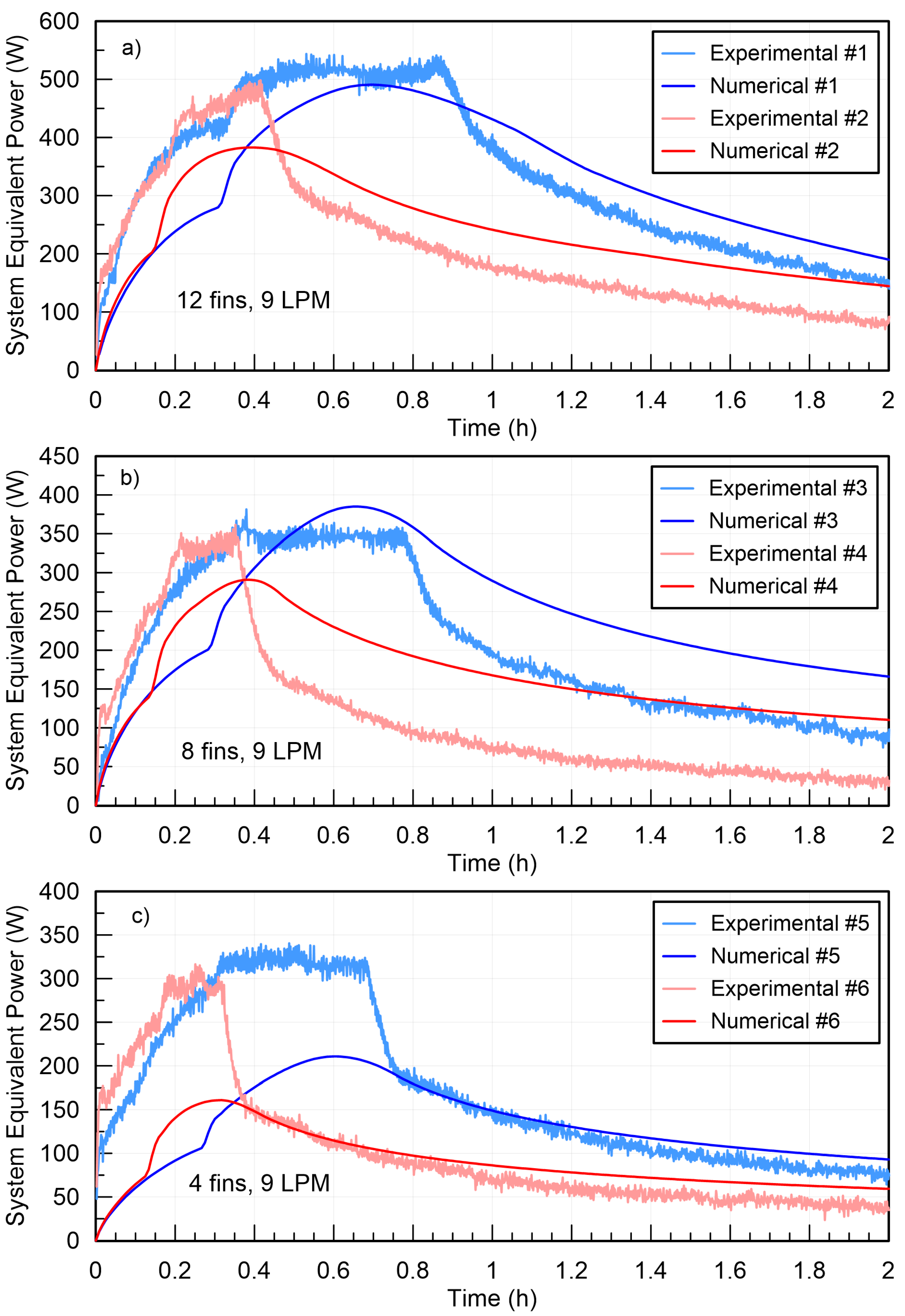
The numerical model was validated using experimental data from the trials using 4, 8, and 12 finned tubes, a flow rate of 9 LPM, and discharging temperature ranges of 65 to 21 °C and 55 to 31 °C. The HTF temperature was also ramped down using trial-specific functions made from the experimental data in Excel to mimic each trial as closely as possible. The simulation time was set to 7200 s with a strict maximum time step of 30 s. Figure 8 shows how the numerical results from this simplified geometry and model compare to the experimental results from Herbinger and Groulx [18].
Based on the experimental conditions of each trial, the HTF convection coefficients inside each finned tube were calculated following the approach presented in Section 3.4. These convection coefficient values are presented in Table 3.
From the validation results, some cases showed great agreement; for example, the validation study 1 (see Table 3 and Figure 8a) for 12 fins was able to capture the maximum power and the representative power decline over time. Others captured general orders of magnitude for the system equivalent power without fully capturing the maximum power. It appears clear that this simplified 2D model is not as accurate or predictive for cases using only four finned tubes. However, for the purpose of this study, the validation results from Figure 8 prove that the simplified 2D models capture enough physics from the process, providing general trends. Therefore, the models were found to be valuable for parametric studies on the impact of the variation in the PCM thermal conductivity in this case.
For reference, during this work, simulations were performed using an Intel Core i7-10700k CPU (3.8 GHz with 5.1 GHz Turbo Boost) and 32 GB of RAM.
4. Results and Discussion
The parametric study performed in this paper looked at varying the thermal conductivity of dodecanoic acid by multiplying both the solid and liquid thermal conductivities by factors of 1, 1.05, 1.1, 1.2, 1.5, 2, 5, 10, 20, and 50, and determining the resulting system equivalent power over time. Simulations were performed for 12-, 8-, and 4-finned-tube geometries, with a system HTF flow rate of 9 LPM and over two sets of initial and final system temperatures: Ti = 65 °C to Tf = 21 °C and Ti = 55 °C to Tf = 31 °C.
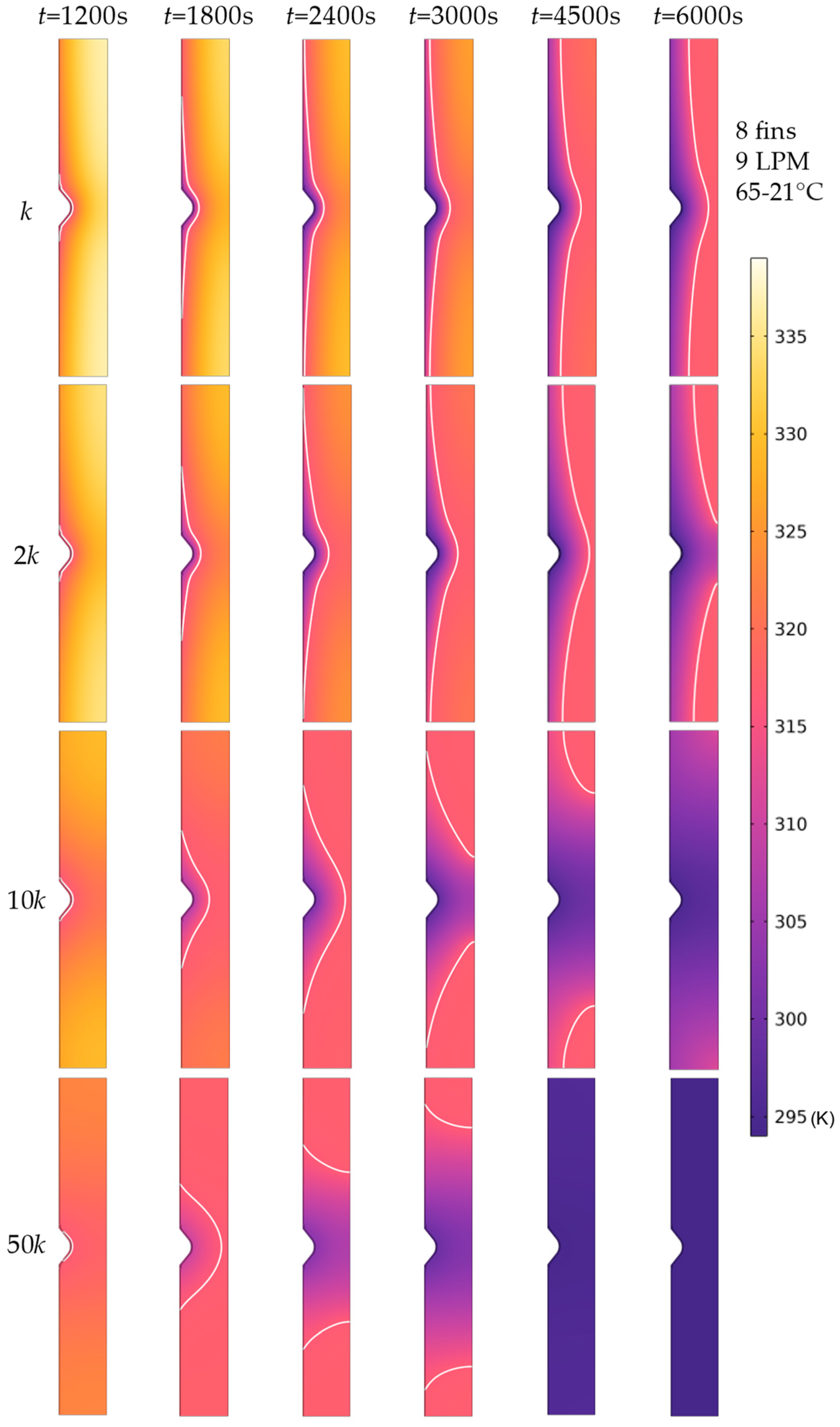
Firstly, Figure 9 shows the temperature distribution, as well as the solidification interface, at six specific times (t = 1200, 1800, 2400, 3000, 4500, and 6000 s) for the original dodecanoic acid, and PCMs with thermal conductivities of 2k, 10k, and 50k obtained in the eight-finned-tube geometry at a starting temperature of 65 °C and discharged with an HTF at 21 °C. In the figure, the solidification interface is indicated by a white line in each image at the phase change temperature of dodecanoic acid (Tm = 43.3 °C = 316.45 K). From the temperature legend, purple and dark-pink colors correspond to temperatures below the phase change temperature and correspond to the PCM being solid; orange and yellow colors correspond to the PCM being liquid.
As expected, solidification started on the surface of the finned tube and progressed away as time went on, with faster solidification around the tube section of the fin compared to solidification from the fins. Therefore, solidification ended at the top and bottom of the system around the symmetry line.
The progression of the solidification interface for the PCM with a thermal conductivity of 2k was very similar to the original dodecanoic acid, although slightly faster, and a solid bridge was created by the time the simulation reached 6000 s. Increasing the thermal conductivity to 10k, the PCM was fully melted by 6000 s. Further increasing the thermal conductivity to 50k, the PCM was fully melted by 4500 s, but it can also be observed that with this increased thermal conductivity, the fins play a lesser role in conducting heat away from the solidifying PCM; the solidification interface is much more centered on the tube. This points to the fact that an increase in the thermal conductivity of the PCM could allow a change in geometry (the removing of fins in this case), reducing the necessary heat exchange material and potentially reducing the initial cost of the TES infrastructure.
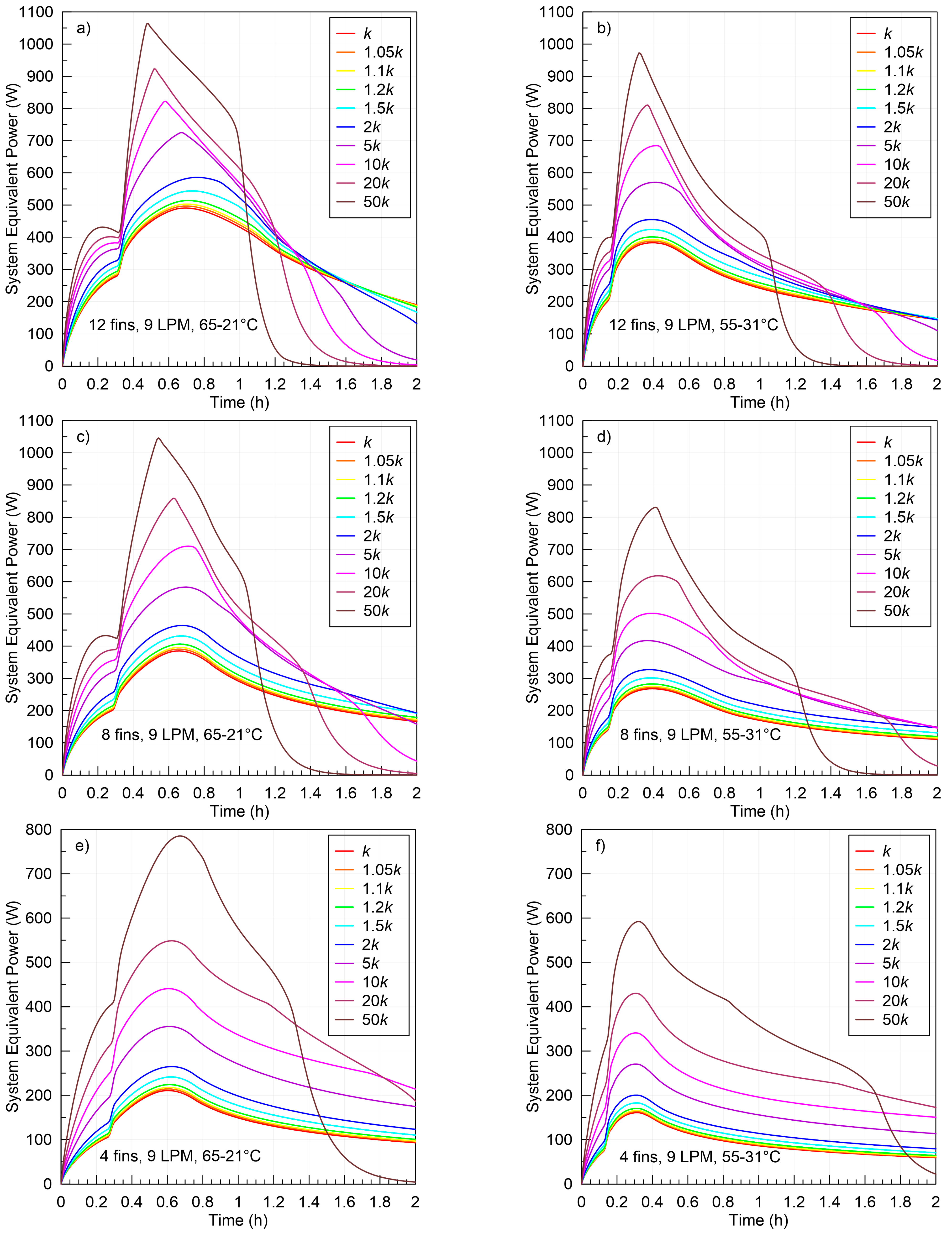
Figure 10 presents the system equivalent power obtained for each finned-tube configuration and operating temperatures for the various PCM thermal conductivity values used in this parametric study. Figure 10a,c,e show the results when the systems were at 65 °C initially and were discharged with an HTF at 21 °C for the 12-, 8-, and 4-finned-tube configurations, respectively. The system with 12 fins always had a larger discharging power compared to the other two. For the original dodecanoic acid (k), the maximum system equivalent power was approximately 500 W for 12 fins, 400 W for 8 fins, and 200 W for 4 fins. Increasing the thermal conductivity to 2k led to a maximum power of approximately 600 W for 12 fins, 450 W for 8 fins, and 260 W for 4 fins. The increase in absolute power was only by approximately 12 to 30%, with a doubling of the PCM thermal conductivity. Finally, increasing the thermal conductivity by a factor of 50 (50k) led to a maximum power of approximately 1075 W for 12 fins, 1050 W for 8 fins, and nearly 800 W for 4 fins. As expected, the increase in thermal conductivity at this point made the number of fins less impactful. An increase in thermal conductivity by a factor of 50 only led to an increase in maximum power by factors of approximately 2.1 to 4. The increase in thermal conductivity was more impactful with fewer finned tubes in the system.
The thermal conductivity increase led to a reduction in the total time needed to fully discharge the system. However, it took an increase in conductivity by a factor of 5 or 10 to bring the discharge time below 2 h, and by a factor of 5 in the case for the four-finned-tube geometry.
Figure 10b,d,f show similar results when the systems were at 55 °C initially and discharged with an HTF at 31 °C. It has been demonstrated that the temperature differential between the HTF driving temperature and the PCM melting temperature plays a crucial role in power extraction [18]. In this case, the HTF temperature being higher led to smaller system equivalent power and a higher difference between power extracted with 12, 8, and 4 fins. For the original dodecanoic acid (k), the maximum power was approximately 375 W for 12 fins, 275 W for 8 fins, and 160 W for 4 fins. For 2k, it was 450 W for 12 fins, 325 W for 8 fins, and 200 W for 4 fins; absolute power increased by approximately 20% to 25% when compared to a standard k. When increased by 50k, the power was 975 W for 12 fins, 825 W for 8 fins, and 600 W for 4 fins.
In this case, the increase in thermal conductivity by a factor of 50 only led to an increase in system equivalent maximum power by factors of approximately 2.6 to 3.8, again with the largest impact of the increase in thermal conductivity being felt with the smaller number of finned tubes.
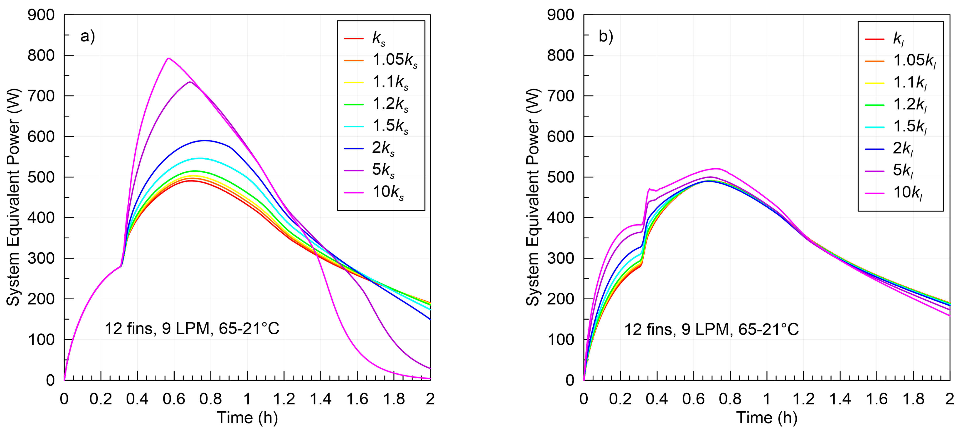
Finally, the numerical model allows studies where just the solid or liquid thermal conductivity of the PCM is changed (with the thermal conductivity of the other phase staying at the original dodecanoic acid value of k). Figure 11a shows the system equivalent power when the liquid thermal conductivity remains at k and only the solid thermal conductivity is increased.
The power remains the same for each scenario until solidification starts (just before reaching the 0.4 h mark), which is consistent with the liquid thermal conductivity being the same for each scenario. In this scenario, the maximum power extraction reaches a value of 800 W when the solid PCM thermal conductivity is 50ks, compared to a maximum value of 1075 W when the conductivity of both phases is 50k, as per Figure 10a.
Figure 11b shows the system equivalent power when the solid thermal conductivity remains at k and only the liquid thermal conductivity is increased. This figure shows the impact of the liquid thermal conductivity when the PCM is entirely liquid prior to solidification (again just before reaching the 0.4 h mark). It was also observed that the liquid thermal conductivity increase on its own plays a very minor role in the overall power extracted from the system. From the information obtained through these studies and the results from Figure 11, it is clear that an increase in the solid PCM thermal conductivity plays the most important role overall, and any increase in the thermal conductivity of the liquid PCM then affirms this increase by further increasing the overall system equivalent power.
5. Conclusions
A numerical study, using a simplified and validated 2D numerical model, looking at the impact of the PCM thermal conductivity on the system equivalent power is presented in this work. The results show that with a substantial thermal conductivity increase of 100% (doubling the thermal conductivity), in the range of some of the best results presented when using nanoparticles, for example, the overall system power only increases by approximately 30% at best. From the power vs. time results, it can be concluded that this increase in the PCM thermal conductivity barely affects the overall system discharge history. Increases in the PCM thermal conductivity of at least 500% to 1000% are required to substantially change the discharging power history, with an ultimate power increase up to 400% for a 5000% increase in thermal conductivity.
It is important to keep in mind that the numerical model used for this analysis is simplified, using a 2D approach to capture the important behaviors of a more complex 3D system. Although the validation shows the similarities in the captured behaviors, it is not perfect, so additional processes might play different roles as the PCM thermal conductivity is increased. It is equally important to keep in mind that this analysis is based on a given system, with a given geometry and operating conditions; the impact of the PCM conductivity could be different for other systems. As mentioned in the introduction, the answer to the simple question related to the impact of the PCM thermal conductivity requires complex work because of the dependence of the heat transfer rates during phase change on much more than that one PCM properties. Additional analysis from the community should look at the impact of the PCM thermal conductivity on other systems, as well as the impact that modifying the thermal conductivity might have on other PCM thermophysical properties like the latent heat, density, and specific heat.
Author Contributions
Conceptualization, D.G.; methodology, M.B. and D.G.; validation, M.B.; formal analysis, M.B.; investigation, M.B.; writing—original draft preparation, M.B.; writing—review and editing, D.G.; visualization, M.B.; supervision, D.G. All authors have read and agreed to the published version of the manuscript.
Funding
This research was funded by the Natural Science and Engineering Research Council (NSERC) of Canada through an Undergraduate Student Research Award (USRA) awarded to M.B.
Data Availability Statement
The raw data supporting the conclusions of this article will be made available by the authors on request.
Conflicts of Interest
The authors declare no conflicts of interest.
References
- Renewables 2023—Analysis and Forecast to 2028; International Energy Agency (IEA): Paris, France, 2024; 143p.
- Letcher, T.M. Storing Energy with Special Reference to Renewable Energy Sources; Elsevier: New York, NY, USA, 2016; 565p. [Google Scholar]
- Cabeza, L.F. Advances in Thermal Energy Storage Systems: Methods and Applications, 2nd ed.; Elsevier: Cambridge, UK, 2021; 775p. [Google Scholar]
- Groulx, D. Design of latent heat energy storage systems using phase change materials. In Advances in Thermal Energy Storage Systems, 2nd ed.; Cabeza, L., Ed.; Elsevier: Cambridge, MA, USA, 2021; pp. 331–357. [Google Scholar]
- Agyenim, F.; Hewitt, N.; Eames, P.; Smyth, M. A review of materials, heat transfer and phase change problem formulation for latent heat thermal energy storage systems (LHTESS). Renew. Sustain. Energy Rev. 2010, 14, 615–628. [Google Scholar] [CrossRef]
- Kalapala, L.; Devanuri, J.K. Influence of operational and design parameters on the performance of a PCM based heat exchanger for thermal energy storage—A review. J. Energy Storage 2018, 20, 497–519. [Google Scholar] [CrossRef]
- Cabeza, L.F.; Castell, A.; Barreneche, C.; de Gracia, A.; Fernández, A.I. Materials used as PCM in thermal energy storage in buildings: A review. Renew. Sustain. Energy Rev. 2011, 15, 1675–1695. [Google Scholar] [CrossRef]
- Noël, J.A.; Kahwaji, S.; Desgrosseilliers, L.; Groulx, D.; White, M.A. Phase Change Materials. In Storing Energy with Special Reference to Renewable Energy Sources, 2nd ed.; Letcher, T.M., Ed.; Elsevier: Cambridge, MA, USA, 2022; pp. 503–535. [Google Scholar]
- Palacios, A.; Cong, L.; Navarro, M.E.; Ding, Y.; Barreneche, C. Thermal conductivity measurement techniques for characterizing thermal energy storage materials—A review. Renew. Sustain. Energy Rev. 2019, 108, 32–52. [Google Scholar] [CrossRef]
- Diarce, G.; Campos-Celador, Á.; Quant, L.; Garcia-Romero, A. A Simple and Fast Methodology for the Design of Plate-Based LHTESS Systems. In Proceedings of the 12th IIR Conference on Phase-Change Materials and Slurries for Refrigeration and Air Conditioning (PCM 2018), Orford, QC, Canada, 21–23 May 2018. [Google Scholar]
- Kuznik, F.; Arzamendia Lopez, J.P.; Baillis, D.; Johannes, K. Design of a PCM to air heat exchanger using dimensionless analysis: Application to electricity peak shaving in buildings. Energy Build. 2015, 106, 65–73. [Google Scholar] [CrossRef]
- Saydam, V.; Parsazadeh, M.; Radeef, M.; Duan, X. Design and experimental analysis of a helical coil phase change heat exchanger for thermal energy storage. J. Energy Storage 2019, 21, 9–17. [Google Scholar] [CrossRef]
- Mehling, H.; Cabeza, L.F. Heat and Cold Storage with PCM; Springer: Berlin, Germany, 2008; 308p. [Google Scholar]
- Gonzalez-Nino, D.; Boteler, L.M.; Ibitayo, D.; Jankowski, N.R.; Urciuoli, D.; Kierzewski, I.M.; Quintero, P.O. Experimental evaluation of metallic phase change materials for thermal transient mitigation. Int. J. Heat Mass Transf. 2018, 116, 512–519. [Google Scholar] [CrossRef]
- White, M.A.; Kahwaji, S.; Noel, J.A. Recent advances in phase change materials for thermal energy storage. Chem. Commun. 2024, 60, 1690–1706. [Google Scholar] [CrossRef] [PubMed]
- Groulx, D. The Rate Problem: Search for Application Specific Optimization of Energy Storage Density and Exchange Rate. In Proceedings of the 12th IIR Conference on Phase-Change Materials and Slurries for Refrigeration and Air Conditioning (PCM 2018), Orford, QC, Canada, 21–23 May 2018. [Google Scholar]
- Agyenim, F.; Eames, P.; Smyth, M. Heat transfer enhancement in medium temperature thermal energy storage system using a multitube heat transfer array. Renew. Energy 2010, 35, 198–207. [Google Scholar] [CrossRef]
- Herbinger, F.; Groulx, D. Experimental comparative analysis of finned-tube PCM-heat exchangers’ performance. Appl. Therm. Eng. 2022, 211, 118532. [Google Scholar] [CrossRef]
- Khanna, S.; Newar, S.; Sharma, V.; Reddy, K.S.; Mallick, T.K. Optimization of fins fitted phase change material equipped solar photovoltaic under various working circumstances. Energy Convers. Manag. 2019, 180, 1185–1195. [Google Scholar] [CrossRef]
- Joybari, M.M.; Haghighat, F.; Seddegh, S.; Al-Abidi, A.A. Heat transfer enhancement of phase change materials by fins under simultaneous charging and discharging. Energy Convers. Manag. 2017, 152, 136–156. [Google Scholar] [CrossRef]
- Vogel, J.; Johnson, M. Natural convection during melting in vertical finned tube latent thermal energy storage systems. Appl. Energy 2019, 246, 38–52. [Google Scholar] [CrossRef]
- Xie, J.; Lee, H.M.; Xiang, J. Numerical study of thermally optimized metal structures in a Phase Change Material (PCM) enclosure. Appl. Therm. Eng. 2019, 148, 825–837. [Google Scholar] [CrossRef]
- Yao, Y.; Wu, H.; Liu, Z.; Gao, Z. Pore-scale visualization and measurement of paraffin melting in high porosity open-cell copper foam. Int. J. Therm. Sci. 2018, 123, 73–85. [Google Scholar] [CrossRef]
- MacDevette, M.M.; Myers, T.G. Contact melting of a three-dimensional phase change material on a flat substrate. Int. J. Heat Mass Transf. 2012, 55, 6798–6807. [Google Scholar] [CrossRef]
- Rozenfeld, T.; Kozak, Y.; Hayat, R.; Ziskind, G. Close-contact melting in a horizontal cylindrical enclosure with longitudinal plate fins: Demonstration, modeling and application to thermal storage. Int. J. Heat Mass Transf. 2015, 86, 465–477. [Google Scholar] [CrossRef]
- Hu, N.; Zhang, R.-H.; Zhang, S.-T.; Liu, J.; Fan, L.-W. A laser interferometric measurement on the melt film thickness during close-contact melting on an isothermally-heated horizontal plate. Int. J. Heat Mass Transf. 2019, 138, 713–718. [Google Scholar] [CrossRef]
- Gunasekara, S.N.; Ignatowicz, M.; Chiu, J.N.; Martin, V. Thermal conductivity measurement of erythritol, xylitol, and their blends for phase change material design: A methodological study. Int. J. Energy Res. 2019, 43, 1785–1801. [Google Scholar] [CrossRef]
- D’Oliveira, E.J.; Pereira, S.C.C.; Groulx, D.; Azimov, U. Thermophysical properties of Nano-enhanced phase change materials for domestic heating applications. J. Energy Storage 2022, 46, 103794. [Google Scholar] [CrossRef]
- Eisapour, M.; Eisapour, A.H.; Shafaghat, A.H.; Mohammed, H.I.; Talebizadehsardari, P.; Chen, Z. Solidification of a nano-enhanced phase change material (NePCM) in a double elliptical latent heat storage unit with wavy inner tubes. Sol. Energy 2022, 241, 39–53. [Google Scholar] [CrossRef]
- Sadrameli, S.M.; Motaharinejad, F.; Mohammadpour, M.; Dorkoosh, F. An experimental investigation to the thermal conductivity enhancement of paraffin wax as a phase change material using diamond nanoparticles as a promoting factor. Heat Mass Transf. 2019, 55, 1801–1808. [Google Scholar] [CrossRef]
- Groulx, D. Numerical Study of Nano-Enhanced PCMs: Are they Worth it? In Proceedings of the 1st Thermal and Fluid Engineering Summer Conference, TFESC, New York, NY, USA, 9–12 August 2015. [Google Scholar]
- Desgrosseilliers, L.; Whitman, C.A.; Groulx, D.; White, M.A. Dodecanoic acid as a promising phase-change material for thermal energy storage. Appl. Therm. Eng. 2013, 53, 37–41. [Google Scholar] [CrossRef]
- Liu, C.; Groulx, D. Experimental study of the phase change heat transfer inside a horizontal cylindrical latent heat energy storage system. Int. J. Therm. Sci. 2014, 82, 100–110. [Google Scholar] [CrossRef]
- Azad, M.; Groulx, D.; Donaldson, A. Solidification of phase change materials in horizontal annuli. J. Energy Storage 2023, 57, 106308. [Google Scholar] [CrossRef]
- Groulx, D.; Biwole, P.H. Solar PV Passive Temperature Control using Phase Change Materials. In Proceedings of the 15th International Heat Transfer Conference (IHTC-15), Kyoto, Japan, 10–15 August 2014. [Google Scholar]
- Ogoh, W.; Groulx, D. Stefan’s Problem: Validation of a One-Dimensional Solid-Liquid Phase Change Heat Transfer Process. In Proceedings of the COMSOL Conference 2010, Boston, MA, USA, 9–7 October 2010. [Google Scholar]
- Kheirabadi, A.C.; Groulx, D. Simulating Phase Change Heat Transfer using COMSOL and FLUENT: Effect of the Mushy-Zone Constant. Comput. Therm. Sci. 2015, 7, 427–440. [Google Scholar] [CrossRef]
- Rohsenow, W.M.; Hartnett, J.P.; Cho, Y.I. Handbook of Heat Transfer, 3rd ed.; McGraw-Hil: Boston, MA, USA, 1998; 1344p. [Google Scholar]
Figure 1.
Pictures of (a) one manufactured finned-tube; (b) twelve finned-tubes attached to the cover of the storage container; (c) 10 kg of dodecanoic acid added in the storage container with the heat exchanger; and (d) sealed storage container with twelve finned tubes (insulation omitted from this photograph) [18].

Figure 2.
Finned-tube geometry; dimensions in mm (thermo-dynamics.com).

Figure 3.
Model geometry and boundary conditions.

Figure 4.
Mesh 2 used for the validation study.

Figure 5.
System equivalent power as a function of time for the 12 fins, 9 LPM, and 65 to 21 °C study for the five meshes used in the mesh independence study.
Figure 5.
System equivalent power as a function of time for the 12 fins, 9 LPM, and 65 to 21 °C study for the five meshes used in the mesh independence study.

Figure 6.
Solidification interface position at 7020s for ΔT = 1, 4, 8, and 12 K (red, blue, green, and orange lines, respectively).
Figure 6.
Solidification interface position at 7020s for ΔT = 1, 4, 8, and 12 K (red, blue, green, and orange lines, respectively).

Figure 7.
System equivalent power as a function of time for the 12 fins, 9 LPM, and 65 to 21 °C study for four mushy-zone temperature intervals: ΔT = 1, 4, 8, and 12 K.
Figure 7.
System equivalent power as a function of time for the 12 fins, 9 LPM, and 65 to 21 °C study for four mushy-zone temperature intervals: ΔT = 1, 4, 8, and 12 K.

Figure 8.
System equivalent power as a function of time for six numerical validation cases compared to experimental results from [18]: (a) 12 finned tubes, (b) 8 finned tubes, and (c) 4 finned tubes. The case numbers are indicated in Table 3 for reference.

Figure 9.
Temperature distribution snapshots at timesteps of 1200 s, 1800 s, 2400 s, 3000 s, 4500 s, and 6000 s for parametric study of 8 finned tubes at an HTF flowrate of 9 LPM, being discharged from 65 to 21 °C, showing thermal conductivities of k, 2k, 10k, and 50k.
Figure 9.
Temperature distribution snapshots at timesteps of 1200 s, 1800 s, 2400 s, 3000 s, 4500 s, and 6000 s for parametric study of 8 finned tubes at an HTF flowrate of 9 LPM, being discharged from 65 to 21 °C, showing thermal conductivities of k, 2k, 10k, and 50k.

Figure 10.
System equivalent power over time as a function of the PCM solid and liquid thermal conductivities from k to 50k for simulations with an HTF flow rate of 9 LPM: 12 finned tubes from (a) 65 to 21 °C and (b) 55 to 31 °C; 8 finned tubes from (c) 65 to 21 °C and (d) 55 to 31 °C; 4 finned tubes from (e) 65 to 21 °C and (f) 55 to 31 °C.

Figure 11.
System equivalent power over time as a function of the PCM: (a) solid thermal conductivity from ks to 10ks (kl constant) and (b) liquid thermal conductivity from kl to 10kl (ks constant) for simulation with 12 fins, 9 LPM, and Ti = 65 °C to Tf = 21 °C.
Figure 11.
System equivalent power over time as a function of the PCM: (a) solid thermal conductivity from ks to 10ks (kl constant) and (b) liquid thermal conductivity from kl to 10kl (ks constant) for simulation with 12 fins, 9 LPM, and Ti = 65 °C to Tf = 21 °C.


Table 1.
Thermophysical properties of dodecanoic acid [32].
Table 1.
Thermophysical properties of dodecanoic acid [32].
| Property | Value |
|---|---|
| cp,s @ 20 °C | 1.95 ± 0.03 kJ/kg∙K |
| cp,l @ 45 °C | 2.4 ± 0.2 kJ/kg∙K |
| ks @ 30°C | 0.160 ± 0.004 W/m∙K |
| kl @ 50 °C | 0.150 ± 0.004 W/m∙K |
| ρs @ 22 °C | 930 ± 20 kg/m3 |
| ρl @ 50 °C | 885 ± 20 kg/m3 |
| Tm | 43.3 ± 1.5 °C |
| L | 184 ± 9 kJ/kg |
Table 2.
Statistics of the meshes used in the mesh independence study.
| Mesh | Domain Elements | Boundary Elements | Total Elements | Average Element Size | Simulation Time |
|---|---|---|---|---|---|
| 1 | 5135 | 888 | 6023 | 0.00090 m | 17 s |
| 2 | 8152 | 985 | 9137 | 0.00057 m | 16 s |
| 3 | 15,419 | 1140 | 16,559 | 0.00046 m | 23 s |
| 4 | 30,907 | 1805 | 32,712 | 0.00030 m | 46 s |
| 5 | 130,768 | 3617 | 134,385 | 0.00013 m | 194 s |
Table 3.
Validation study and convection coefficients used.
| Validation Study | # of Fins | (L/min) | ||
|---|---|---|---|---|
| 1 | 12 | 9 | 65 to 21 | 1590.32 |
| 2 | 12 | 9 | 55 to 31 | 1624.05 |
| 3 | 8 | 9 | 65 to 21 | 1953.44 |
| 4 | 8 | 9 | 55 to 31 | 2285.66 |
| 5 | 4 | 9 | 65 to 21 | 3809.42 |
| 6 | 4 | 9 | 55 to 31 | 4180.27 |
Disclaimer/Publisher’s Note: The statements, opinions and data contained in all publications are solely those of the individual author(s) and contributor(s) and not of MDPI and/or the editor(s). MDPI and/or the editor(s) disclaim responsibility for any injury to people or property resulting from any ideas, methods, instructions or products referred to in the content. |
© 2024 by the authors. Licensee MDPI, Basel, Switzerland. This article is an open access article distributed under the terms and conditions of the Creative Commons Attribution (CC BY) license (https://creativecommons.org/licenses/by/4.0/).
Share and Cite
MDPI and ACS Style
Belinson, M.; Groulx, D. Numerical Study of a Latent Heat Storage System’s Performance as a Function of the Phase Change Material’s Thermal Conductivity. Appl. Sci. 2024, 14, 3318. https://doi.org/10.3390/app14083318
AMA Style
Belinson M, Groulx D. Numerical Study of a Latent Heat Storage System’s Performance as a Function of the Phase Change Material’s Thermal Conductivity. Applied Sciences. 2024; 14(8):3318. https://doi.org/10.3390/app14083318
Chicago/Turabian StyleBelinson, Maxim, and Dominic Groulx. 2024. "Numerical Study of a Latent Heat Storage System’s Performance as a Function of the Phase Change Material’s Thermal Conductivity" Applied Sciences 14, no. 8: 3318. https://doi.org/10.3390/app14083318
Note that from the first issue of 2016, this journal uses article numbers instead of page numbers. See further details here.