Design and Experiment of Variable-Spray System Based on Deep Learning

Abstract

In response to issues of the low pesticide-utilization rate caused by the traditional constant spraying method, a variable-spraying system for wheat-field weeds was proposed in this study based on real-time segmentation by deep learning. In this study, the weed density within the operational area was obtained by using the improved DeepLab V3+ semantic segmentation mode, and a variable spray-level model based on real-time weed density and speed was constructed by using PWM variable-spraying technology to adjust the spray volume. The lightweight MobileNet V2 network was selected as its backbone network, and the CA attention mechanism was integrated into the feature extraction module. The mean intersection over the union (MIoU) and mean pixel accuracy (MPA) of the improved DeepLab V3+ were 73.34% and 80.76%, respectively, and the segmentation time for a single image was 0.09 s. The results of field verification tests showed that (1) compared with constant spraying, variable spraying can increase droplet density and save the amount of pesticides, with the droplet density increased by 38.87 droplets/cm² and the pesticide consumption saved by 46.3%; and (2) at the same speed, the average droplet-coverage rate in the areas with sparse weed density decreased by 13.98% compared with the areas with dense weeds. Under the same plant density, the average coverage rate of 0.5 m/s increased by 2.91% and 6.59% compared with 1 m/s and 1.5 m/s, respectively. These results further demonstrated that the system can automatically adjust the spray volume based on different travel speeds and weed densities. This research can provide theoretical and reference support for the development of new precision-spray plant-protection machinery for wheat fields.

1. Introduction

Weeds compete with field crops for water, nutrients, light, and space resources, negatively affecting crop growth and yields [1,2,3]. To effectively control weeds, chemical herbicides are used to eliminate weeds and improve the crop growth environment and yields [4,5,6]. However, traditional agricultural herbicide spraying involves spraying herbicide in a large area in the same amount, without considering weed density and crop variability. The residual herbicide will lead to problems such as environmental pollution and serious human health issues [7,8,9]. Variable-spraying technology is based on the actual growth situation and demand of crops to realize the online adjustment and variable spraying of pesticide dosage [10,11,12]. Variable-spraying technology can effectively reduce the consumption of pesticides, thereby reducing the runoff and leakage of pesticides [13].

In recent years, deep learning technology has been widely applied in variable spraying. Hussain N et al. [14] developed an intelligent variable sprayer using YOLOv3-tiny, which was used to spray pesticides on potato crops. Moreover, 42% and 43% of pesticides were saved in weed- and simulated diseased plant-detection experiments, respectively, by using SVRS. Zhao DJ et al. [15] proposed a vision tracking method based on machine vision to meet the requirements of precision spraying large-spaced crops. The experimental results showed that the target spray error was less than or equal to 6.5 mm, and the target precision spraying was realized. De Castro AI et al. [16] used machine learning and the color index to distinguish weeds in fields based on multi-spectral images of farmland. The results showed that 71.7%~95.4% and 4.3%~12% of herbicides were saved in the untreated areas and low-herbicide-dosage areas, respectively. Xu YL et al. [17] designed a variable-spraying system that identified the crops in the field and between the ridges based on machine vision and adjusted the spray flow by adjusting the spray width of the sprayer. The experiment results indicated that the error between the spray amount of the variable-spraying system and the theoretical value was less than 10%. Partel V et al. [18] created and evaluated a cost-effective intelligent sprayer using a laboratory-scale YOLO model of spraying agricultural chemicals on weeds. It was reported that the accuracy of using different Nvidia GPUS ranged from 40% to 90%. In summary, some research has been conducted on variable-spray technology, but there is little research on the variable spraying of wheat.

In this study, the weed density in wheat fields was analyzed in real time based on variable-spraying techniques with visual sensors, and a variable-spraying flow-regulation model, with real-time weed density and the unit speed as the control variables, was established. Firstly, based on an improved DeepLab V3+ semantic segmentation model, the weed density in the field was obtained in real time. Secondly, based on the flow-regulation model, a system-performance test experiment was conducted. Finally, the effectiveness of the variable-spraying system was verified by field tests, and under different speed conditions, more spraying was realized in the areas with dense weeds; less spraying was realized in the areas with sparse weeds; and no spraying was realized in the areas without weeds. This provided a reference for the application of variable-spraying technology in wheat fields in field-wheat production.

2. Materials and Methods

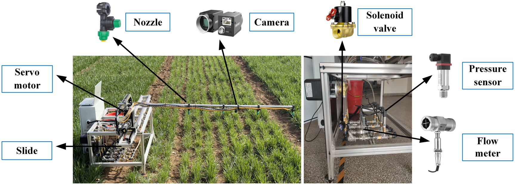
2.1. Variable-Spray System for Wheat Weeds

The main components of the variable-spray system in this study are shown in Figure 1. The whole test-bench spray system can be divided into two parts: a semantic segmentation system and a spray control system.

A HIKVISION MV-CA050-11UC (Hikvision, Hangzhou, China) camera was used to capture HD-quality video at 35 fps, and the test data were stored on a laptop. The spray controller was mainly controlled by a PLC (Programmable Logic Controller, XINJE, Wuxi, China). Pressure sensors and turbine flow meters were installed in four separate lines to measure the pressure and flow rate of each branch of the spray test bench. The spray boom was installed at a height of 1.2 m from the ground. The length of the spray boom was 2 m. A group of spraying devices was installed every 50 cm on the spray bar, with a total of four groups of spraying devices. Each spray device was equipped with a standard solid fan nozzle and a solenoid valve. The length of the test bench was 2 m. The speed of the spray boom was controlled by the servo motor. The PWM duty cycle of the corresponding solenoid valve of each nozzle was calculated by the spray system based on the speed and weed density. Through RS485 communication, real-time application instructions were sent by the upper computer to the lower computer’s PLC. The spraying flow of the nozzles was adjusted by the PLC of the lower unit according to the received PWM duty cycle, enabling variable spraying. The spray flow chart of the variable-spray system is shown in Figure 2.

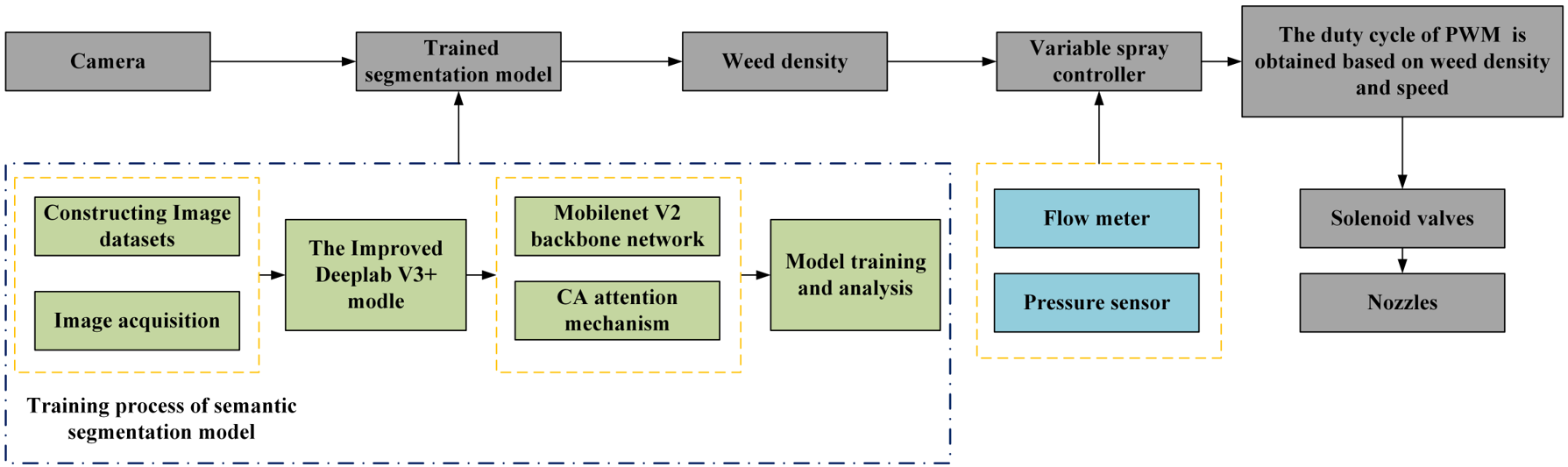
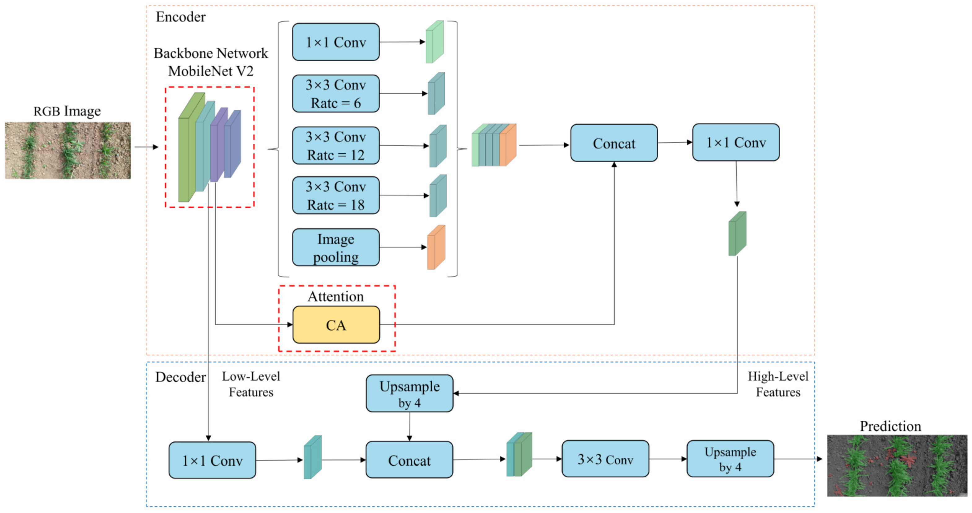
2.2. Semantic Segmentation Model for Wheat Weeds Based on DeepLab V3+

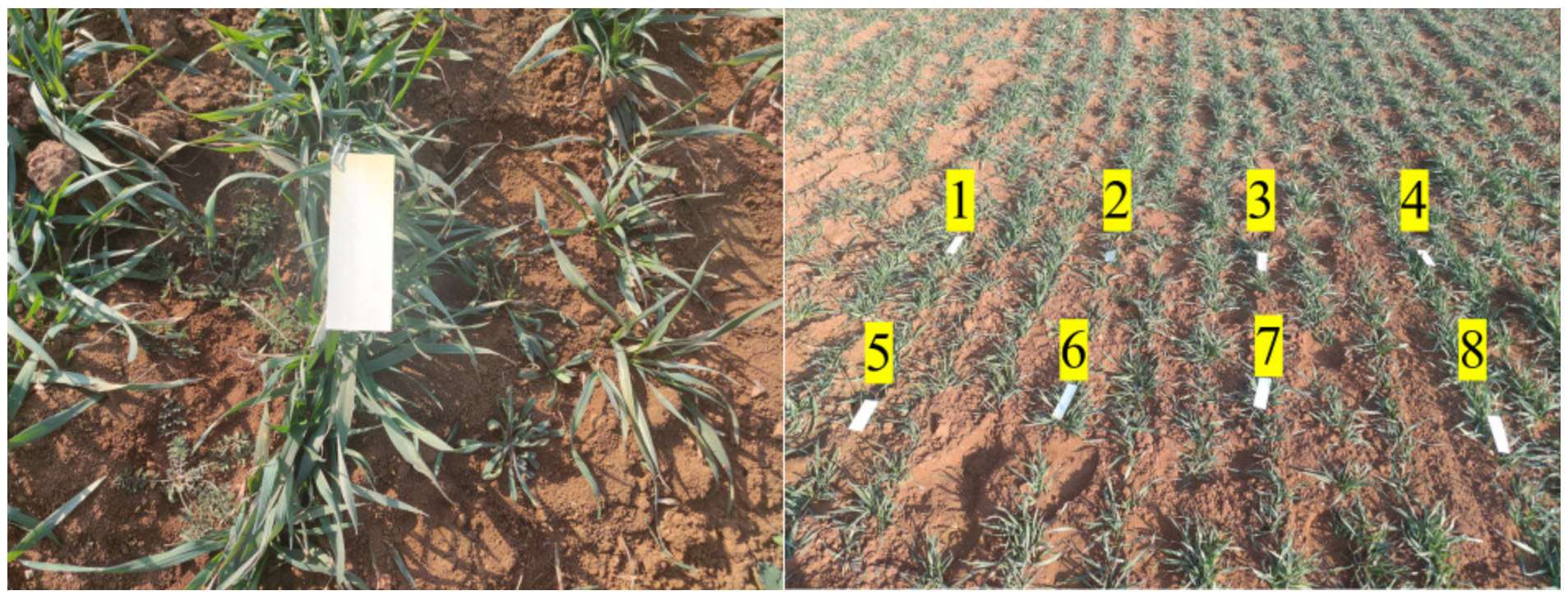
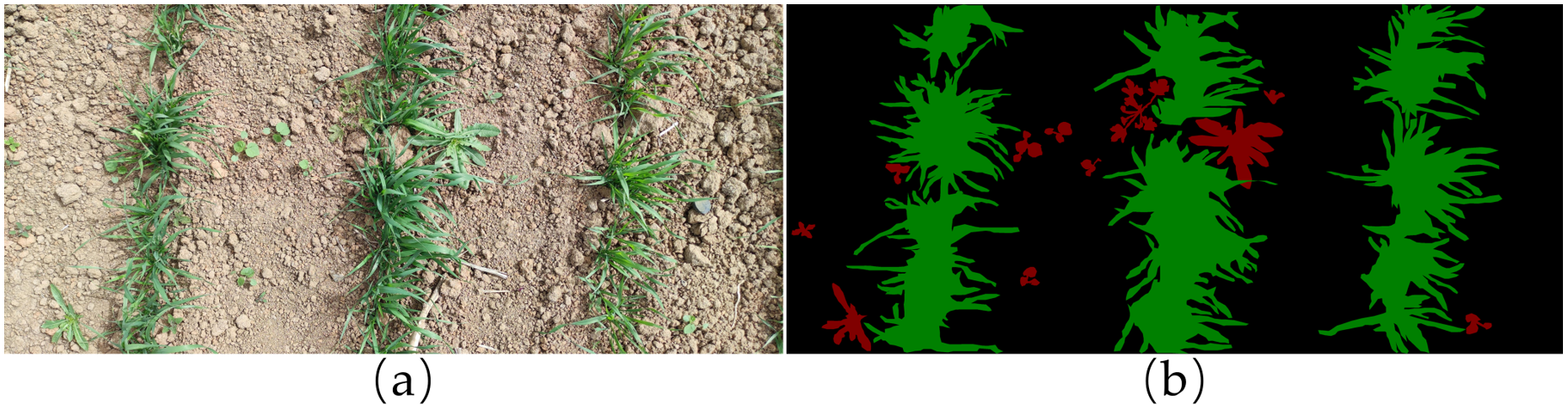
2.2.1. Data Acquisition

The data acquisition interval was from 26 March to 1 April 2023. The collection site was the Smart Agriculture Demonstration Farm, Yiyang County, Luoyang City, Henan Province, China. A total of 620 images of wheat weeds, each with a size of 5184 × 3450 pixels, was captured with the Canon EOS 60D camera at a distance of 50 cm from the vertical ground under different light intensities. To reduce the computational workload during model training, the image size was compressed to 512 × 512 pixels.

Each image was manually annotated via the LabelMe annotation tool (LabelMe, V4.5.13, Computer science and artificial intelligence laboratory, Massachusetts institute of technology, USA), with the resulting labels being formatted in JSON after annotation. The JSON files were then converted into the mask label image, where, as depicted in Figure 3b, red areas represented weeds and green areas signified wheat. Methods such as mirror flipping and brightness adjustment were used to increase the amount of training data and the generalization ability of the model. The enhanced sample data were allocated to a training set of 1500 images, a test set of 500 images, and a validation set of 500 images, according to a distribution ratio of 6:2:2.

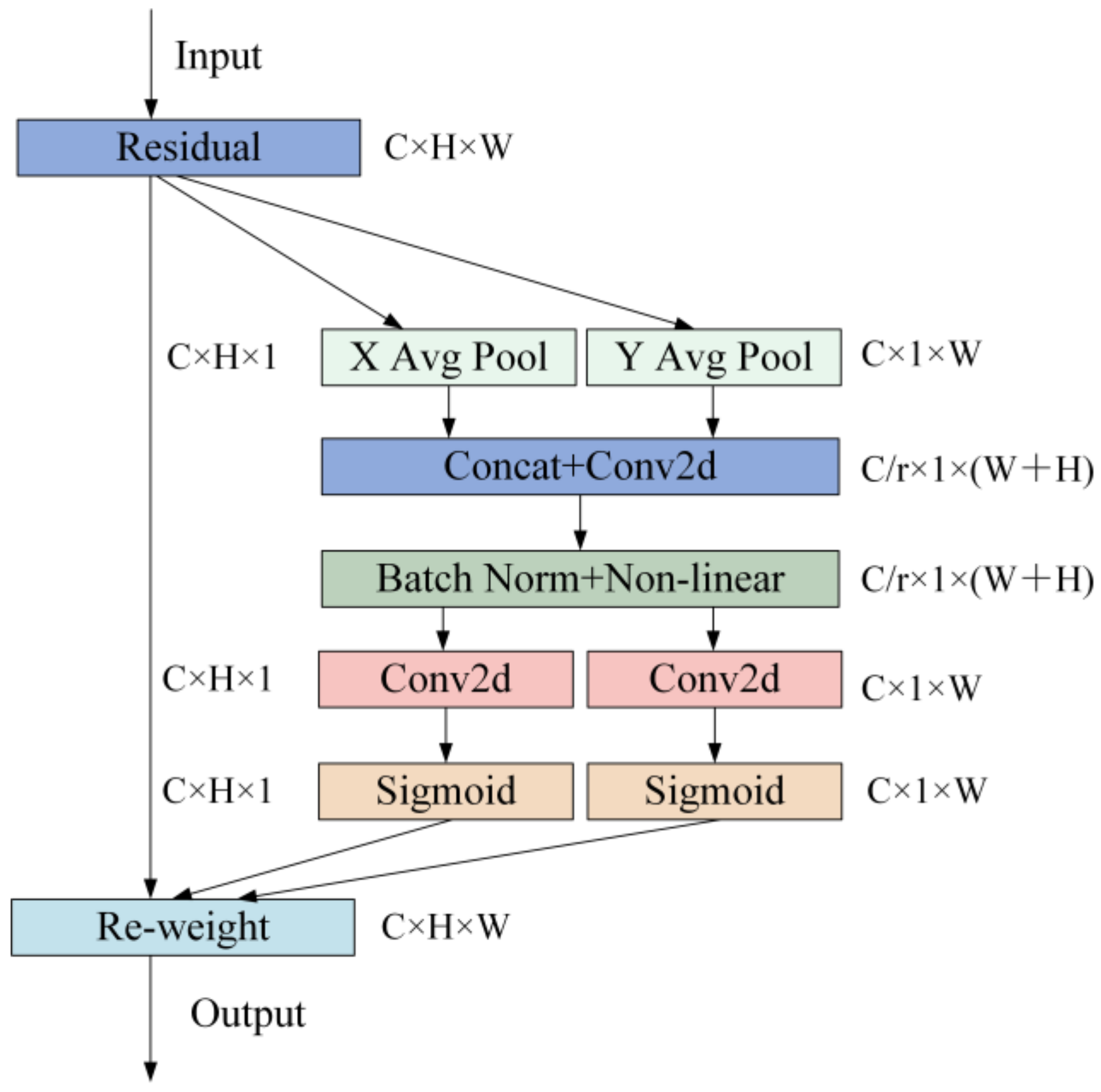
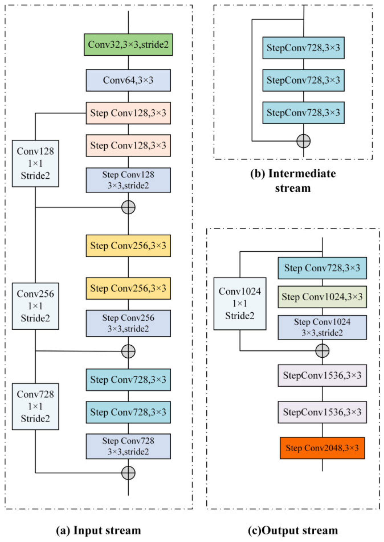
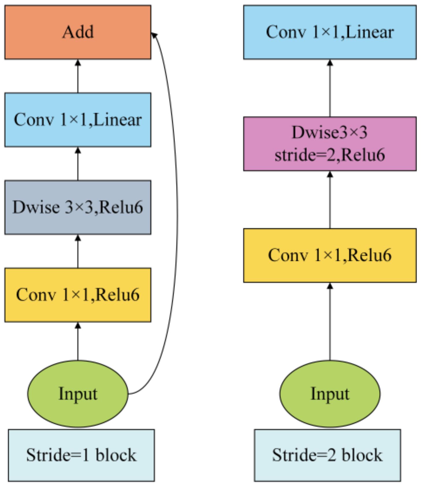
2.2.2. Improved DeepLab V3+ Segmentation Model

The DeepLab V3+ [19] encoder incorporates null-space pyramid pooling with the Xception network [20] as the feature extraction network. Depth-separable convolution was introduced for improvement within the ASPP (Atrous Spatial Pyramid Pooling) module. A multigrid method with different expansion rates was employed by the encoder across the three convolutions. The resulting image-level features were fed into a 1 × 1 convolution of 256 filters and batch-normalized [21]. The decoder module was designed to establish connections between low-level and high-level features. A depth-separable convolution was also applied in the decoder part. The feature layer obtained from the output of the encoder (high-level features, with an outstride of 16) emerged after four-fold bilinear upsampling with the feature layer corresponding to the same resolution in the encoder (low-level features, with an outstride of 4) after 1 × 1 product dimensionality reduction. Subsequently, 3 × 3 convolutional refinement was performed, followed by another four-fold bilinear upsampling to obtain the prediction results at the original image resolution [22,23].

The Xception model was constructed from a linear stack of deeply separable convolutions with residual connections. It consisted of an Entry flow, a Middle flow that is repeated 16 times, and an Exit flow [24]. The Xception network architecture is illustrated in Figure 4. After batch normalization, a 1 × 1 convolution was performed, and the channels were downscaled to obtain the output of the encoder part.

However, the features in the Entry flow in the Xception component were not sufficiently downsampled and had a high resolution. Additionally, the Entry flow contained a large number of channels, leading to substantial GPU memory consumption. As a consequence, Xception incurred heavy computational demands and consumed considerable time [25].

Variable-spraying systems require real-time sensing of the environment to quickly implement spray control decisions. However, the Xception network suffers from a large memory footprint and high computational requirements, resulting in a slow detection speed. It is unable to meet the requirements for use on the devices of variable-spray control systems.

Therefore, the lightweight MobileNet V2 network [26] was selected in this study as the backbone network of the DeepLab V3+ semantic segmentation model for feature extraction. The MobileNet V2 network architecture is illustrated in Figure 5.

The MobileNet V2 network mainly employs depthwise separable convolutions and introduces the inverted residual structure and the linear bottleneck structure. In the structure of the residual proposed by Resnet [27], the dimension reduction was first achieved using 1 × 1 convolution, followed by 3 × 3 convolution, and finally, dimension uplift through 1 × 1 convolution. In the inverted residual structure of MobileNet V2, the order of dimension reduction and uplift was reversed, and the 3 × 3 convolution was replaced with the 3 × 3 DW convolution. The linear bottleneck layer design of MobileNet V2 consists of depthwise separable convolutions and inverted residual structures.

As shown in Figure 5, when stride = 1, the input first expands the number of channels through a 1 × 1 convolution, with RelU6 as the activation function; then, it passes through a 3 × 3 depthwise convolution with RelU6 as the activation function, and after the number of channels is compressed back by 1 × 1 pointwise convolution, the activation function is linear. Finally, the shortcut is used to add the two results together. The feature graph compressed by 1 × 1 convolution is concatenated with the input as the next bottleneck block. When stride = 2, the input and output feature map sizes are different; thus, the shortcut connection is not utilized.

As the depth of a neural network increases, the vanishing gradient problem tends to occur. The inverted residual structure can effectively alleviate this problem. Therefore, when the network layer number is shallow, MobileNet V2 uses a bottleneck block without residuals, where the stride is set to 2. As the number of network layers increases, MobileNet V2 uses a bottleneck block with residuals to alleviate the phenomenon of disappearing gradients, where the stride is set to 1.

The linear bottleneck structure improves the nonlinear representation of the network by introducing extension and projection layers, enabling the model to better capture complex features in the input data while reducing computational cost. By restricting the dimensions and the quantity of parameters involved in the convolution operation, the model’s lightweight and high efficiency was maintained. The overall parameter count and computational demand of the model were reduced by the MobileNet V2 network. This enhancement can boost the speed of semantic segmentation and is well-suited for deployment on mobile devices.

Due to the diverse background of weeds and wheat growth in fields, the model can focus on extracting weed features from the images by adding an attention mechanism, thereby reducing the interference of environmental factors. In this study, the CA attention module [28] was incorporated into the encoder part of DeepLab V3+, which ran in parallel with the ASPP. The encoder was optimized by splicing the outputs of the two parts and adjusting the number of channels. This optimization enhanced the model’s ability to segment the details of weed edges, thereby improving overall segmentation performance and accuracy. The structure of the CA attention network is shown in Figure 6. The CA attention network decomposed channel attention into two one-dimensional feature-encoding processes, each of which aggregated features along two spatial directions [29]. The resulting feature maps were then encoded as a pair of directional and positional attention maps, respectively. This can be used as a complement to the input feature maps to improve the representation of the attentional object.

In the improved DeepLab V3+ model, the lightweight MobileNet V2 network model was used to replace the original Xception network with large parameters as the backbone network, which reduced the parameter count of the model and addressed issues of spatial details loss and insufficient feature extraction. The CA attention module was introduced, and it was added in parallel with the ASPP after the feature extraction network, which enhanced the network’s ability to capture global contextual feature information and improved the model’s segmentation accuracy of the edges of weeds. The structure of the improved model is depicted in Figure 7.

2.2.3. Model Training Environment and Parameter Setting

The TensorFlow deep learning framework was used in this experiment. The hardware devices used had the following configuration and installed software: an Intel Core i7-6700 CPU @ 3.40 GHz × 8 threads, 16GB RAM, GeForce GTX TITAN X GPU with 12GB RAM, 500GB mechanical hard drive, NVIDIA driver version 390.87, CUDA version 9.0. 390.87, CUDA version 9.0.176, CUDNN 7.0.5 neural network acceleration library, a Linux Ubuntu 18.04 LTS operating system, Python version 3.8, and TensorFlow version 1.8.0.

The loss function L is the cross-entropy loss function. The number of training iterations was set to 30,000, the impulse was set to 0.9, and the initial learning rate was set to 0.01. The Poly strategy was adopted; the batch size was set to 4, and it was validated every 100 iterations and saved as the latest training model; and the model with the highest accuracy of preservation was finally selected.

2.2.4. Segmentation Performance Evaluation Index

To evaluate the segmentation results and compare the performance of the model. IoU, MIoU, and MPA were used as the evaluation criteria of the segmentation model. IoU is the intersection over the union. MIoU is the mean intersection over the union; it represents the mean ratio of the intersection and union of the two sets of true values and predicted values for each category. MPA is the mean pixel accuracy; it represents the proportion of the total number of correctly classified pixels in each category averaged to the total number of that category. The formulas are shown below:

$$IoU=\frac{P_{ii}}{{\displaystyle {\sum }_{j=0}^k{P}_{ij}}+{\displaystyle {\sum }_{j=0}^k{P}_{ji}-P_{ii}}}$$

(1)

$$MIoU=\frac{1}{k+1}{\displaystyle {\sum }_{i=0}^k\frac{P_{ii}}{{\displaystyle {\sum }_{j=0}^k{P}_{ij}}+{\displaystyle {\sum }_{j=0}^k{P}_{ji}-P_{ii}}}}$$

(2)

$$MPA=\frac{1}{k+1}{\displaystyle {\sum }_{i=0}^k\frac{P_{ii}}{{\displaystyle {\sum }_{j=0}^k{P}_{ij}}}}$$

(3)

where P_ii denotes the number of pixels belonging to category i and predicted to be i; P_ij denotes the number of pixels belonging to category i but predicted to be j; P_ji denotes the number of pixels belonging to category j but predicted to be i. k + 1 denotes the number of segmentation categories; i is the true value; and j is the predicted value.

2.3. Variable-Spray Regulation Decision

The variable-spray control system is used mainly to determine the spray level of each nozzle using weed density and the forward speed of the spray bar. In this study, PWM variable-spray technology was used; a spray volume model with duty cycle, flow rate, density data, and speed was established; a spray level decision-making method was designed; and the transformation of the flow level was realized.

(1)

Calculation method of weed density.

To obtain the weed density, the captured images were divided into two rows × four columns in the system, and the percentage of weed pixels in each region was calculated. The percentage of pixels obtained represents the density of weeds in each region division. The density of weeds in each region can be expressed as follows:

$$D=\frac{A_i}{A}$$

(4)

where A_i denotes the area covered by weeds in the area and A is the total area. A_i and A can be run in correlation with pixel points of the image as a substitute.

(2)

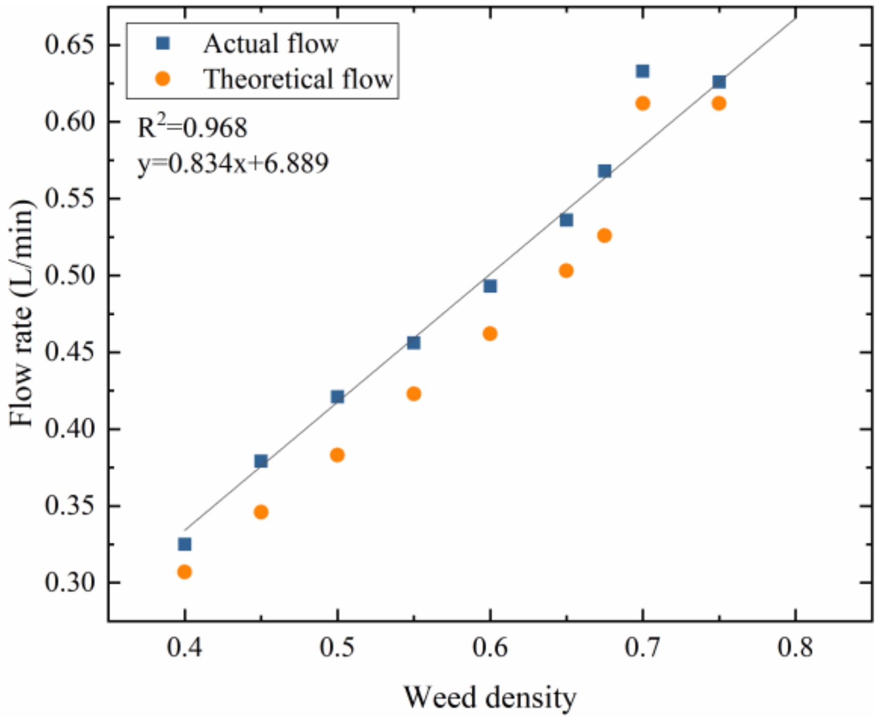
The impact of weed density on the flow rate.

The nozzle flow rate needs to be matched with the weed density, and the required amount of spray per unit of weed density is a set value, which is related to the type of drug to be sprayed and the target to be sprayed. Based on the above conditions, the formula for calculating the amount of chemical required for normal spraying per unit area is

$$u=\frac{q}{60wv}$$

(5)

where u is the amount of drug required for normal spraying in the unit area in L/m². q is the nozzle flow rate in ml/min. w is the width of a single nozzle in m, and v is the speed of travel in m/s.

In this study, the nozzle flow rate q used is 615 mL/min, and the standard traveling speed v is set to 1 m/s. The width w of a single nozzle is selected to be 0.5 m, and u is 0.0205 L/m² from Equation (5).

In the actual spraying process, the density of weeds is different in different plots. The amount of drug required per unit area under weed cover D is

$$Q=\frac{Du}{k}$$

(6)

where Q is the dose required per unit area in L/m² and k is the maximum weed cover during the spraying period.

(3)

The impact of speed on flow rate.

The relationship between the amount of chemical per unit area Q and the speed v is expressed as

$$Q=\frac{q}{60wv}$$

(7)

From Equations (6) and (7), it can be derived that

$$q=\frac{60Dwvu}{k}$$

(8)

In the actual spraying process, two variables—weed density D and speed v—affect the spray rate, and it is necessary to finally determine the spray-rating decision according to these two variables.

(4)

Nozzle-flow duty-cycle flow curve.

PWM adjusts the actual flow rate of the nozzle by controlling the duty cycle of the solenoid valve’s opening and closing times [30]. Taking into account the uniformity of spraying and the response effect of the solenoid valve during actual debugging, the PWM control frequency of the solenoid valve was set to 5 Hz. Wei Xinhua et al. [31] found that when the duty cycle is low, with the increase in spraying pressure, the response effect of the solenoid valve will become worse and the spraying effect will be seriously distorted. After the nozzle model, the system spray pressure, solenoid valve model, and PWM control signal frequency and other conditions are determined, and the flow rate and duty cycle of the PWM signal are calibrated. The linear equation between the nozzle flow rate and the PWM duty cycle is

$$q=As+b$$

(9)

where A represents the slope of the flow-duty cycle curve at a specific pressure and frequency, b is the intercept of the flow-duty cycle curve, and s is the duty cycle.

The pressure of the spray system was 0.4 MPa. A single-factor linear fitting method was employed to establish the corresponding relationship model between the duty cycle and the nozzle spray flow rate. In the calibration process, flow rates were determined for each PWM duty cycle by adjusting the PWM duty cycle settings. After calibration, it was found that the coefficient of determination of the model was 0.91, indicating a strong linear relationship between the nozzle flow rate and the duty cycle when the duty cycle varies from 20% to 80%. Thus, at a pressure of 0.4 MPa, the flow rate curve of each nozzle with the duty cycle can be represented as q = 0.00393 s + 0.217.

(5)

Spray-rating decision model.

Based on the formula of the nozzle flow rate, speed, and plant density per unit area, the relationship between the theoretical duty cycle and weeds in a unit area can be derived by combining Equations (8) and (9). Calibration yields A = 0.00393 and b = 0.217, and the formula is shown as follows:

$$s=\frac{60Dwvu-0.217k}{0.00393k}$$

(10)

Due to varying speeds at each moment, the weed density obtained from each frame of the image is different. To reduce the frequency of the duty cycle changes, the theoretical duty cycle was divided into corresponding levels through the decision value in this paper. During the calibration process, it was found that with multiple nozzles, the flow rate varied by less than 5% and remained essentially constant for duty cycles greater than 80%, while the flow rate was smaller for duty cycles less than 20%. In this study, when the duty cycle is less than 20%, the duty cycle is set to 0, and the solenoid valve is closed. When the duty cycle is between 20% and 80%, the duty cycle is calculated according to the spray flow model. If the duty cycle exceeds 80%, the corresponding duty cycle is set to 100%. The spray flow model is as follows:

$$\left\{\begin{array}{l}s=0,s<20\\ s=\frac{60Dwvu-0.217k}{0.00393k},20\le s\le 80\\ s=100,s>80\end{array}\right.$$

(11)

2.4. Experimental Design and Methodology

2.4.1. System Performance Verification Tests

Before the field test, due to the comprehensive response ability of the control system and hardware, there may be some variability between the actual and theoretical spray volume of each nozzle. Therefore, a test was conducted to verify whether there is a linear relationship between the actual and theoretical spray volumes for each nozzle.

To ignore variability between nozzles, in this study, Nozzle 1 was randomly selected as the test nozzle, and water was used instead of pesticide. The marching speed of the sprayer was set to 1 m/s in the lower computer program, while the simulated weed density was set in the upper computer program. The weed densities were set to 0.40, 0.45, 0.5, 0.55, 0.6, 0.65, 0.7, and 0.75, respectively, for three simulated tests. The flow rate from Nozzle 1 was calibrated individually before each test. The flow rate of Nozzle 1 was collected with a graduated cylinder continuously for 60 s.

2.4.2. Variable-Spray Experiment

To verify the actual variable spraying effect in the field, the spraying experiments were conducted in Luoyang City, Henan Province, in December 2023. Wheat was used as the experiment subject, with plant heights ranging from 40 to 80 mm. The average ambient temperature during the test ranged from 12 °C to 20 °C. To ensure safety during the spraying process, water was used instead of the drug solution. The spray pressure in the test was set at 0.4 MPa.

According to the growth of wheat weeds, water-sensitive papers were placed 0.5 m apart between the wheat target areas on the shelf. To verify the effect of variable spraying, the distance between the vertical water-sensitive paper placement points should be greater than 0.45 m. Two groups of targets were set up, with four targets in each group. The paper clips were used to fix the water-sensitive test paper onto the wheat or weeds. The water-sensitive test papers were numbered from left to right as numbers 1 to 8, where 1, 2, 7, and 8 were placed in sparse weed areas and 3, 4, 5, and 6 were in dense weed areas. The schematic of partial water-sensitive test-paper placement is shown in Figure 8.

(1)

In the pre-test, the optimal spray speed of the test stand was 1 m/s Therefore, the speed of the spray test was set to 1 m/s and the travel distance was 2 m. Firstly, the test stand conducted three constant spray tests at a speed of 1 m/s. After completing the constant spray experiment, three variable-spray experiments were performed at the same speed.

(2)

Variable-spray experiments were conducted at speeds of 0.5 m/s, 1 m/s, and 1.5 m/s, and three variable-spray experiments were conducted at the same speed, resulting in a total of nine variable-spray experiments.

After each experiment, water-sensitive papers were sequentially removed using disposable gloves and stored in a sealed box to protect them from moisture. The water-sensitive papers were scanned using an HP MPF M479dw printer with integrated scanning, generating PNG images at a resolution of 600 dpi. Spray coverage parameters on individual water-sensitive papers were analyzed using DepositScan droplet analysis software. The final results of the test were obtained as the average of the results of several experiments.

3. Results and Discussion

3.1. Analysis of Segmentation Models

3.1.1. Performance Analysis of Different Models

To validate the effectiveness of the improved DeepLab V3+ model for the extraction of semantic information about wheat and weeds, the classical semantic segmentation models SegNet, UNet, and DeepLabV3+ were introduced for comparative analysis in this research. The model performance was evaluated using IoU, MIoU, MPA, and single-image processing time.

Table 1. Comparison of performance parameters of different semantic segmentation models.

Model	IoU/%			MIoU/%	MPA /%	Segmentation Time/s
	Background	Wheat	Weed
SegNet	80.56	70.23	41.36	64.05	71.53	0.15
UNet	81.24	71.41	50.36	67.57	74.32	0.13
DeepLab V3+	83.38	73.44	53.12	69.98	77.34	0.12
Proposed	84.87	77.28	57.87	73.34	80.76	0.09

shows the comparison of performance parameters of different semantic segmentation models. The IoU of all models for weed segmentation is lower than the corresponding index for background and wheat segmentation. This is because the area of weeds in the dataset in this study is small, which is more difficult to segment compared to the larger areas of the background and wheat. The IoU values of the improved DeepLab V3+ model for weeds and wheat are 57.57% and 77.28%, respectively, which are increased by 4.75% and 3.84% compared to DeepLab V3+. As shown in Table 1, the improved DeepLab V3+ outperforms the comparison models in all evaluation metrics. Compared to SegNet, UNet, and DeepLab V3+, the MIoU values improved by 9.25%, 5.77%, and 3.36%, respectively. The MPA improved by 9.23%, 6.44%, and 3.42%, respectively. These results indicate that the improved DeepLab V3+ model provides better guidance for variable-spraying decisions.

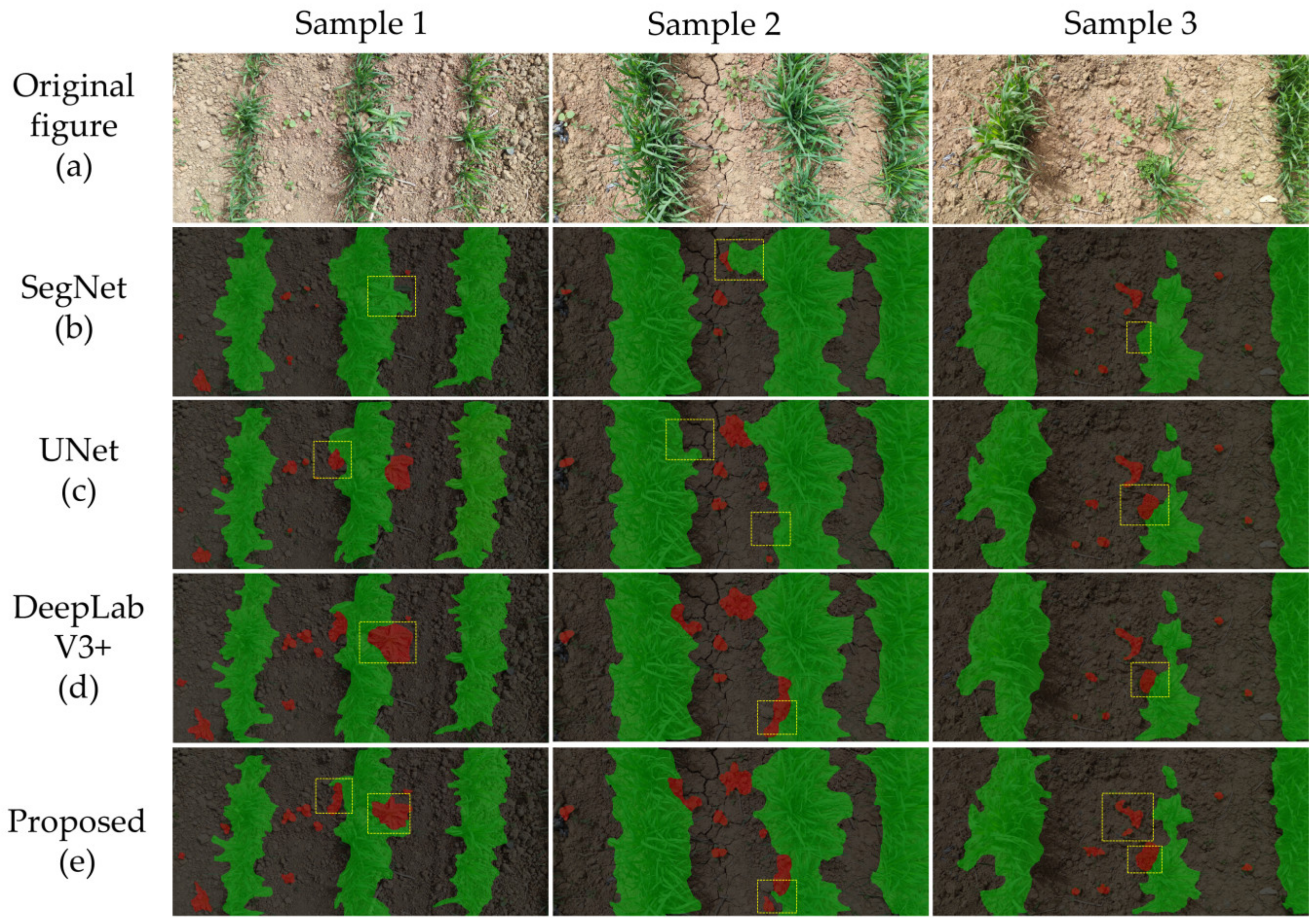
3.1.2. Analysis of Segmentation Results from Different Models

The comparative segmentation results of the improved DeepLab V3+ model with different models are shown in Figure 9. In the figure, the red area represents weeds, the green area represents wheat, and the yellow boxed area indicates regions incorrectly segmented by the model.

As shown in Figure 9b, the SegNet model is inaccurate in weed recognition, and the images of weeds cannot be accurately segmented under conditions of obstruction. As in Figure 9c, the UNet model shows inaccurate segmentation at the intersection of wheat and weeds, and it also fails to completely segment the image of weeds at the intersection. In Figure 9d, the DeepLab V3+ model accurately classifies wheat and weeds but does not entirely segment the image of the unobstructed weeds areas. From Figure 9e, we can observe that the improved DeepLabV3+ model proposed in this paper can segment weeds completely and accurately, and the segmentation effect is more refined in the details of the weed edges. It indicated that the improved model is accurate and superior in weed segmentation and has the characteristics of strong robustness and good generalization performance.

3.2. System Performance Test Results and Analysis

The actual and theoretical spray flow rates corresponding to different weed densities are shown in Figure 10. The actual flow rate range of Nozzle 1 is from 0.32 to 0.61 L/min at the different simulated weed densities. When the weed density is greater than 0.40, the linear fitting R² between the actual flow and the theoretical flow of the Nozzle 1 is 0.968.

The results indicate that the actual flow rate of the system is close to the theoretical flow rate, demonstrating the good real-time performance of the program and consistency in hardware response capability.

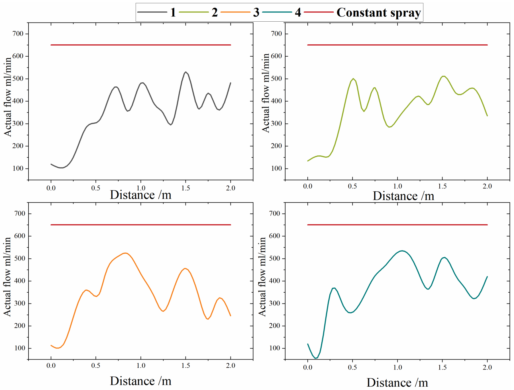
3.3. Variable-Spray Experiment Results

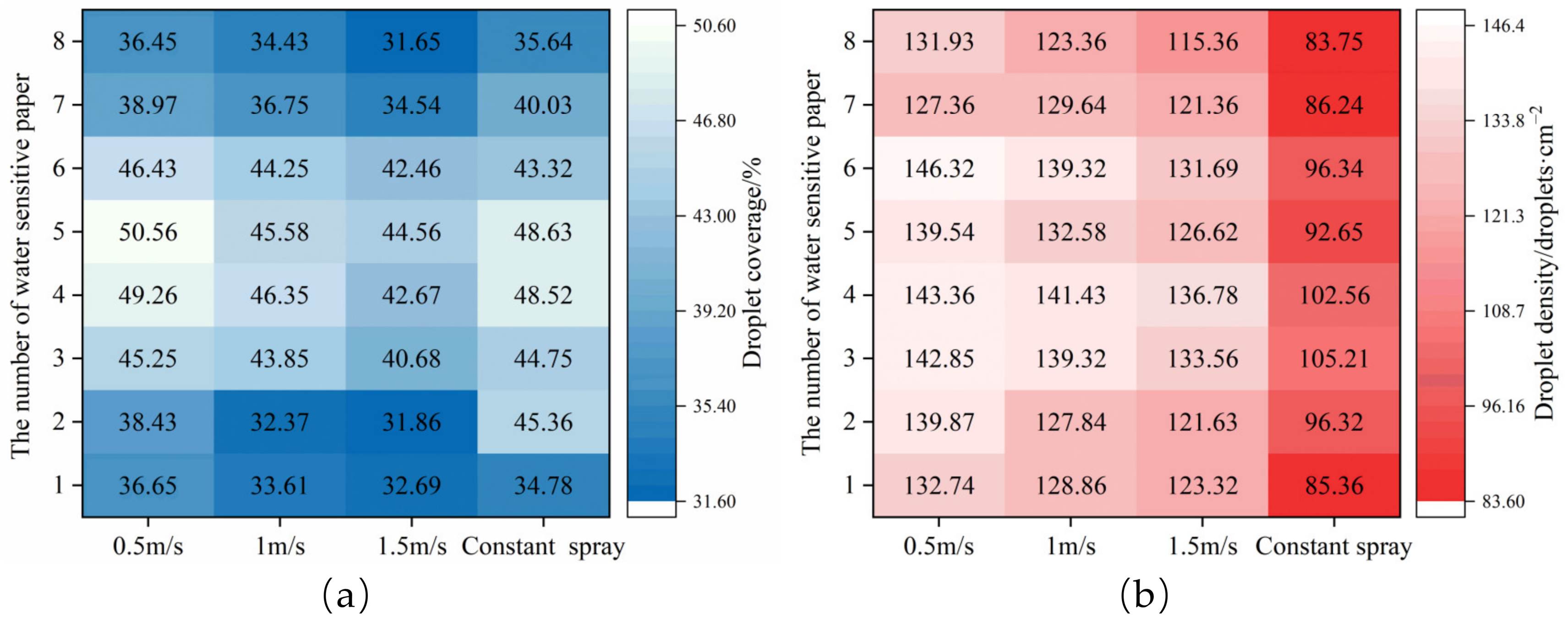
3.3.1. Comparative Analysis of Variable-Spray and Constant-Spray Test Results

Under the speed of 1 m/s, using water-sensitive test paper No. 4 as the sampling point, the parameters of droplets under two spraying modes can be obtained. The results are shown in Figure 11. According to the relevant standard NYT 650-2013, the droplet density should not be less than 30 droplets/cm², and the coverage rate should not be less than 33%. The coverage of droplets was chosen as the evaluation criterion.

Table 2. Droplet parameters under two types of spray methods.

Spraying Modes	VMD/μm	Droplet Density /(Droplets/cm2)	Coverage/%	Deposition Rate /(μL·cm−2)
Constant spray	284.49	102.56	48.52	2.36
Variable spray	146.36	141.43	46.35	2.17

shows that the median volume diameter of variable-spray drops decreases by 138.13 μm, and the density of droplets increases by 38.87 droplets/cm². There is no significant difference in droplet coverage and deposition between the variable and constant sprays under the premise of meeting the evaluation criteria. However, the droplet diameter was refined. The reason for this is that the spraying volume in the constant spray exceeds the actual demand. This excess led to the re-coalescence of atomized droplets after reaching the blade surface, resulting in large droplet sizes. In contrast, variable spraying will not result in excessive spraying, thereby improving the droplet size and spatial distribution of the liquid.

Figure 12 depicts the comparison of the flow rates of the four nozzles under the variable-spray and constant-spray comparison experiments. The red horizontal line represents the constant spray flow rate, while each curve represents the rate of change of the variable-spray flow for each nozzle. The difference between the red horizontal line and each curve represents the amount of spray saved. Compared to constant spraying, the spray volumes were saved by 47%, 44.5%, 49.4%, and 44%, respectively, with an average spray volume reduction of 46.3%. This represents a 4.3% increase in pesticide savings over the variable spraying in weed detection proposed by Hussain N et al. [14].

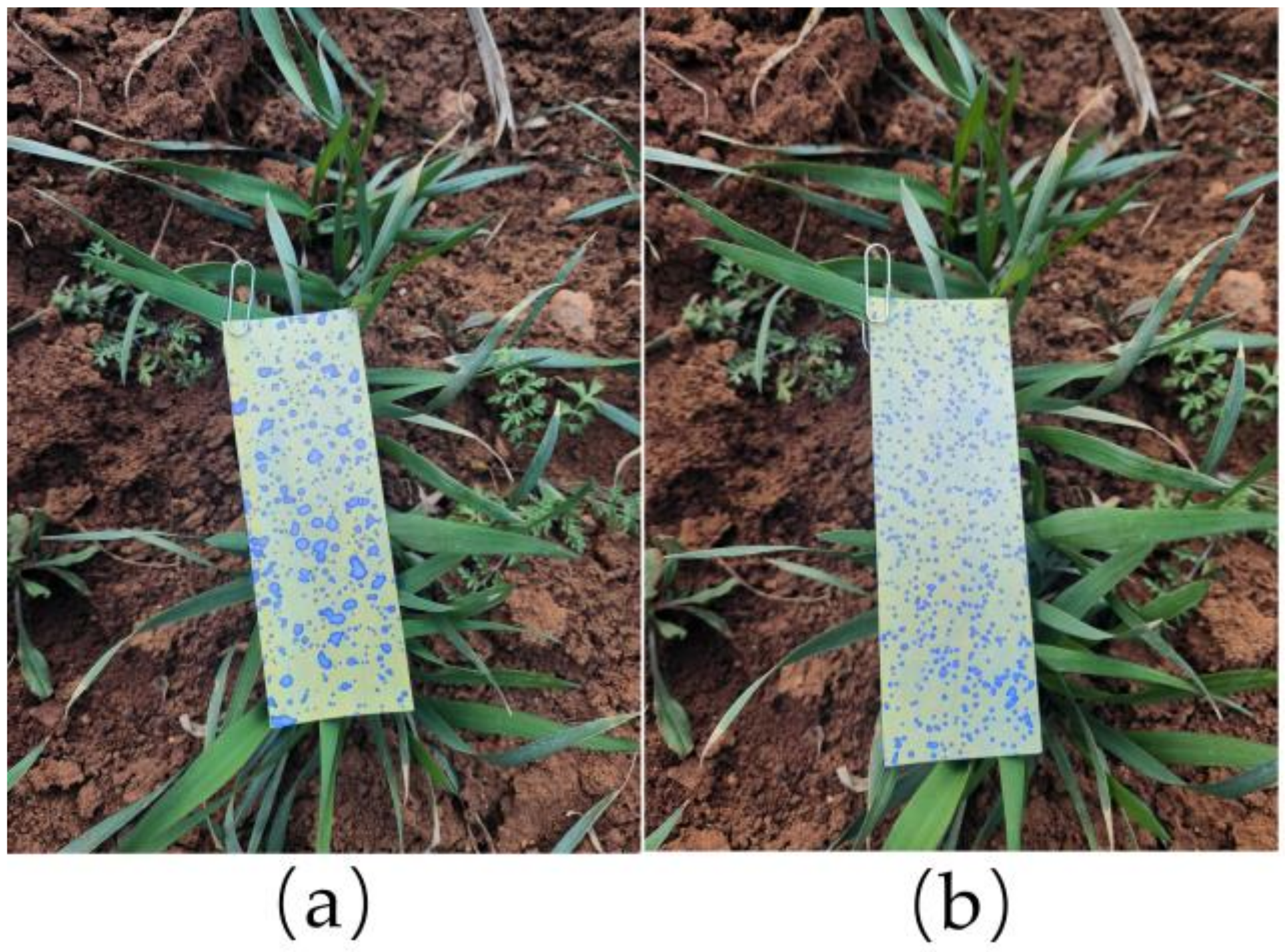
3.3.2. Analysis of Spray Droplet Deposition Effect

The results of the variable-spray droplet-coverage test at different speeds of variable spray are shown in Figure 13a. Taking water-sensitive papers No. 2 and No. 4 as sample data, it could be concluded that at the speed of 1 m/s, the average droplet coverage in areas with sparse weed density decreased by 13.98% compared to areas with dense weeds. Taking water-sensitive paper No. 4 as an example, it showed that under the same plant density, the average coverage rate increased by 2.91% at a forward speed of 0.5 m/s compared to 1 m/s, and was 6.59% higher than the average coverage at 1.5 m/s. There was no significant difference in the coverage rate of droplets between constant and variable sprays in the target area, indicating that variable spraying with less spray volume can achieve good coverage. Variable spraying provides superior spraying performance and can avoid excessive pesticide spraying. Similar research results were also obtained by Yan CG et al. [32] for the variable spraying of grapevines, but the drop-coverage loss in the variable-spray system proposed in this study is 2.17%.

As shown in Figure 13b, the droplet density of the variable spray is significantly higher than that of the constant spray. The average droplet-coverage density of the variable spray is 141.43 droplets/cm². The similarity of sprayed droplets in the process of variable spraying was high according to the field analysis. The droplets undergo secondary collisions in the air. Therefore, finer and more evenly distributed droplets are produced, which leads to an increase in droplet density. These results indicate that the variable-spray system can improve droplet size and spatial distribution uniformity and realize variable spraying at different speeds and different weed densities, with good spraying performance.

4. Conclusions

In this study, weed density was calculated based on the improved DeepLab V3+ semantic segmentation model, and a variable spraying-level model based on real-time weed density and machinery speed was constructed for variable-spraying experimental research. The main conclusions are as follows:

(1)

The overall parameter count and computational load were reduced by the improved model, and the accuracy of image segmentation was enhanced. By substituting the original Xception backbone network with the lightweight MobileNet V2 network and integrating the CA attention mechanism module, the results indicated that the MIoU and MPA of the modified model were 73.34% and 80.76%, respectively, with a single-image segmentation time of 0.09 s.

(2)

Within a certain distance, the atomization parameters of droplets sprayed at the same speed by constant and variable spraying were compared. The results indicated that variable spraying can refine droplet diameter and increase droplet density. The median volume diameter decreased by 138.13 μm, and the droplet density increased by 38.87 droplets/cm², with an average drug-saving rate of 46.3%.

(3)

By utilizing PWM variable-spraying technology, online variable spraying was achieved for different weed densities and speeds. At the same speed, the average droplet-coverage rate in sparse-weed areas decreased by 13.98% compared to dense areas. Under the same plant density, the average coverage rate at a forward speed of 0.5 m/s increased by 2.91% and 6.59% compared with 1 m/s and 1.5 m/s, respectively. The results indicated that, under the standards of spraying, the spray system can automatically adjust the spray volume based on different travel speeds and weed densities, exhibiting excellent spray performance.

References

1. Hamuda, E.; Glavin, M.; Jones, E. A Survey of Image Processing Techniques for Plant Extraction and Segmentation in the Field. Comput. Electron. Agric. 2016, 125, 184–199. [Google Scholar] [CrossRef]
2. Christensen, S.; Søgaard, H.T.; Kudsk, P.; Nørremark, M.; Lund, I.; Nadimi, E.S.; Jørgensen, R. Site-Specific Weed Control Technologies. Weed Res. 2009, 49, 233–241. [Google Scholar] [CrossRef]
3. Veeranampalayam Sivakumar, A.N.; Li, J.; Scott, S.; Psota, E.; Jhala, A.J.; Luck, J.D.; Shi, Y. Comparison of Object Detection and Patch-Based Classification Deep Learning Models on Mid-to Late-Season Weed Detection in UAV Imagery. Remote Sens. 2020, 12, 2136. [Google Scholar] [CrossRef]
4. Wang, A.; Zhang, W.; Wei, X. A Review on Weed Detection Using Ground-Based Machine Vision and Image Processing Techniques. Comput. Electron. Agric. 2019, 158, 226–240. [Google Scholar] [CrossRef]
5. Shaner, D.L.; Beckie, H.J. The Future for Weed Control and Technology. Pest Manag. Sci. 2014, 70, 1329–1339. [Google Scholar] [CrossRef]
6. Lechenet, M.; Dessaint, F.; Py, G.; Makowski, D.; Munier-Jolain, N. Reducing Pesticide Use While Preserving Crop Productivity and Profitability on Arable Farms. Nat. Plants 2017, 3, 17008. [Google Scholar] [CrossRef] [PubMed]
7. Green, J.M. Current State of Herbicides in Herbicide-Resistant Crops. Pest Manag. Sci. 2014, 70, 1351–1357. [Google Scholar] [CrossRef] [PubMed]
8. Myers, J.P.; Antoniou, M.N.; Blumberg, B.; Carroll, L.; Colborn, T.; Everett, L.G.; Hansen, M.; Landrigan, P.J.; Lanphear, B.P.; Mesnage, R.; et al. Concerns over Use of Glyphosate-Based Herbicides and Risks Associated with Exposures: A Consensus Statement. Environ. Health 2016, 15, 19. [Google Scholar] [CrossRef]
9. Gerhards, R.; Sökefeld, M.; Timmermann, C.; Kühbauch, W.; Williams, M.M. Site-Specific Weed Control in Maize, Sugar Beet, Winter Wheat, and Winter Barley. Precis. Agric. 2002, 3, 25–35. [Google Scholar] [CrossRef]
10. Wen, S.; Zhang, Q.; Deng, J.; Lan, Y.; Yin, X.; Shan, J. Design and Experiment of a Variable Spray System for Unmanned Aerial Vehicles Based on PID and PWM Control. Appl. Sci. 2018, 8, 2482. [Google Scholar] [CrossRef]
11. Xiongkui, H. Research Progress and Developmental Recommendations on Precision Spraying Technology and Equipment in China. Smart Agric. 2020, 2, 133. [Google Scholar]
12. Nackley, L.L.; Warneke, B.; Fessler, L.; Pscheidt, J.W.; Lockwood, D.; Wright, W.C.; Sun, X.; Fulcher, A. Variable-Rate Spray Technology Optimizes Pesticide Application by Adjusting for Seasonal Shifts in Deciduous Perennial Crops. HortTechnology 2021, 31, 479–489. [Google Scholar] [CrossRef]
13. Abbas, I.; Liu, J.; Faheem, M.; Noor, R.S.; Shaikh, S.A.; Solangi, K.A.; Raza, S.M. Different Sensor Based Intelligent Spraying Systems in Agriculture. Sens. Actuators Phys. 2020, 316, 112265. [Google Scholar] [CrossRef]
14. Hussain, N.; Farooque, A.A.; Schumann, A.W.; McKenzie-Gopsill, A.; Esau, T.; Abbas, F.; Acharya, B.; Zaman, Q. Design and Development of a Smart Variable Rate Sprayer Using Deep Learning. Remote Sens. 2020, 12, 4091. [Google Scholar] [CrossRef]
15. Zhao, D.J.; Zhang, B.; Wang, X.L.; Guo, H.H.; Xu, S.B. Automatic Target of Indoor Spray Robot Based on Image Moments. Trans. CSAM 2016, 47, 22–29. [Google Scholar]
16. de Castro, A.I.; Jurado-Expósito, M.; Peña-Barragán, J.M.; López-Granados, F. Airborne Multi-Spectral Imagery for Mapping Cruciferous Weeds in Cereal and Legume Crops. Precis. Agric. 2012, 13, 302–321. [Google Scholar] [CrossRef]
17. Xu, Y.L.; Bao, J.L.; Fu, D.P.; Zhu, C.Y. Design and Experiment of Variable Spraying System based on Multiple Combined Nozzles. Trans. CSAE 2016, 32, 47–54. [Google Scholar]
18. Partel, V.; Kakarla, S.C.; Ampatzidis, Y. Development and Evaluation of a Low-Cost and Smart Technology for Precision Weed Management Utilizing Artificial Intelligence. Comput. Electron. Agric. 2019, 157, 339–350. [Google Scholar] [CrossRef]
19. Chen, L.-C.; Papandreou, G.; Schroff, F.; Adam, H. Rethinking Atrous Convolution for Semantic Image Segmentation. arXiv 2017, arXiv:1706.05587. [Google Scholar]
20. Chollet, F. Xception: Deep Learning with Depthwise Separable Convolution. In Proceedings of the 2017 IEEE Conference on Computer Vision and Pattern Recognition (CVPR), Honolulu, HI, USA, 21–26 July 2017; pp. 1251–1258. [Google Scholar]
21. Diab, A.; Kashef, R.; Shaker, A. Deep Learning for LiDAR Point Cloud Classification in Remote Sensing. Sensors 2022, 22, 7868. [Google Scholar] [CrossRef]
22. Baheti, B.; Innani, S.; Gajre, S.; Talbar, S. Semantic Scene Segmentation in Unstructured Environment with Modified DeepLabV3+. Pattern Recognit. Lett. 2020, 138, 223–229. [Google Scholar] [CrossRef]
23. Liu, H.; Jiang, J.B.; Shen, Y.; Jia, W.D.; Zeng, X.; Zhuang, Z.Z. Multi-category Segmentation of Orchard Scene Based on Improved DeepLab V3+. Trans. CSAM 2022, 53, 255–261. [Google Scholar]
24. Peng, H.; Xue, C.; Shao, Y.; Chen, K.; Xiong, J.; Xie, Z.; Zhang, L. Semantic Segmentation of Litchi Branches Using DeepLabV3+ Model. IEEE Access 2020, 8, 164546–164555. [Google Scholar] [CrossRef]
25. Cai, C.; Tan, J.; Zhang, P.; Ye, Y.; Zhang, J. Determining Strawberries’ Varying Maturity Levels by Utilizing Image Segmentation Methods of Improved DeepLabV3+. Agronomy 2022, 12, 1875. [Google Scholar] [CrossRef]
26. Sandler, M.; Howard, A.; Zhu, M.; Zhmoginov, A.; Chen, L.-C. Mobilenetv2: Inverted Residuals and Linear Bottlenecks. In Proceedings of the 2018 IEEE/CVF Conference on Computer Vision and Pattern Recognition (CVPR), Salt Lake City, UT, USA, 18–23 June 2018; pp. 4510–4520. [Google Scholar]
27. Targ, S.; Almeida, D.; Lyman, K. Resnet in Resnet: Generalizing Residual Architectures. arXiv 2016, arXiv:1603.08029. [Google Scholar]
28. Hou, Q.; Zhou, D.; Feng, J. Coordinate Attention for Efficient Mobile Network Design. In Proceedings of the 2021 IEEE/CVF Conference on Computer Vision and Pattern Recognition (CVPR), Nashville, TN, USA, 20–25 June 2021; pp. 13708–13717. [Google Scholar]
29. Liu, K.; Peng, L.; Tang, S. Underwater Object Detection Using TC-YOLO with Attention Mechanisms. Sensors 2023, 23, 2567. [Google Scholar] [CrossRef]
30. Giles, D. Pulse Width Modulation for Nozzle Flow Control: Principles, Development and Status of the Technology. Asp. Appl. Biol. 2020, 144, 59–66. [Google Scholar]
31. Wei, X.H.; Yu, D.Z.; Bai, J.; Jiang, S. Static Spray Deposition Distribution Characteristics of PWM-based Intermittently Spraying System. Trans. CSAE 2013, 29, 19–24. [Google Scholar]
32. Yan, C.; Xu, L.; Yuan, Q.; Ma, S.; Niu, C.; Zhao, S. Design and Experiments of Vineyard Variable Spraying Control System Based on Binocular Vision. Trans. CSAE 2021, 37, 13–22. [Google Scholar]
Figure 1. Composition of variable-spray control system.
Applsci 14 03330 g001
Figure 2. Overall flow chart of the variable-spray system.
Applsci 14 03330 g002
Figure 3. Original and labeled images. (a) Original image; (b) labeled image.
Applsci 14 03330 g003
Figure 4. Xception network structure diagram. (a) Input stream; (b) Intermediate stream; (c) Output stream.
Applsci 14 03330 g004
Figure 5. MobileNet V2 network architecture diagram.
Applsci 14 03330 g005
Figure 6. Coordinate Attention structure diagram.
Applsci 14 03330 g006
Figure 7. Diagram of the improved DeepLab V3+ network structure.
Applsci 14 03330 g007
Figure 8. Partial water-sensitive test paper placement diagram. Water-sensitive test papers numbered 1, 2, 7, and 8 are placed in the sparse weed areas and 3, 4, 5, and 6 are placed in the dense weed areas.
Applsci 14 03330 g008
Figure 9. Comparison of segmentation results of different models. (a) Original figure; (b) SegNet; (c) UNet; (d) DeepLab V3+; (e) Proposed.
Applsci 14 03330 g009
Figure 10. Linear fit of actual spray volume to theoretical spray volume.
Applsci 14 03330 g010
Figure 11. Constant- and variable-spray effect images. (a) Constant spray; (b) variable spray.
Applsci 14 03330 g011
Figure 12. Comparison chart of actual flow rate versus theoretical flow rate.
Applsci 14 03330 g012
Figure 13. Map of droplet coverage and droplet density. (a) Droplet coverage; (b) droplet density.
Applsci 14 03330 g013