Tidal Effects on the Schumann Resonance Amplitudes Recorded by the Global Coherence Monitoring System

Abstract

The main scientific result of this paper is the demonstration of the fact that tidal effects induced by the Moon affect the Schumann resonance amplitudes measured at magnetometers located at different geographical locations of the Global Coherence Monitoring System. Each magnetometer is paired with the closest monitoring station of the global tidal wave measurement network. This paper introduces the Schumann Resonance Complexity Index (SRCI), computed by using the calibrated H-rank algorithm on the local magnetic field data recorded by each magnetometer of the Global Coherence Monitoring System. Tidal wave data recorded at each monitoring station are also used to compute the Tidal Wave Complexity Index (TWCI). Eliminating diel cycles from the SRCI data yields significant statistical correlations between the SRCI and TWCI data, proving the hypothesis of tidal effects on the global network of magnetometers.

1. Introduction

In 1949, J. Bartels introduced the planetary Kp index, derived from three-hourly K indices specific to observatories [1]. This planetary geomagnetic K index assesses geomagnetic activity within three-hourly UTC (Coordinated Universal Time) intervals on a quasi-logarithmic scale from 0 to 9. This geomagnetic Kp index quantifies disturbances in the Earth’s magnetic field caused by solar activity [2]. The Kp index is derived from observations of magnetic field variations at specific geomagnetic observatories around the world [1]. These observations are used to calculate a single global index that represents the overall level of geomagnetic activity. The Kp index is particularly useful for assessing the potential impact of space weather events, such as solar flares and coronal mass ejections, on Earth’s magnetosphere. Monitoring the Kp index is important for space weather forecasting and for assessing the potential impacts on various technological systems on Earth. The Kp index is then derived by combining the individual K-values from different observatories. The overall Kp index is a global measure of geomagnetic activity during a specific three-hour period.

Every day the 24 h Kp index is calculated by summing the Kp values over eight consecutive 3 h intervals. The Kp index is calculated on a semi-logarithmic scale, while its counterpart is calculated on a linear scale and is known as the Ap index. The daily sum of the Ap index is calculated by summing the eight three-hour Ap index values. This helps provide a smoother representation of the overall geomagnetic activity for a full day [1]. It provides a daily measure of geomagnetic activity, and its values are related to the disturbance storm time (Dst) index, which measures the globally averaged strength of the Earth’s geomagnetic field disturbance. The Dst index was proposed by M. Sugiura in 1964 [3] to measure the magnitude of the current that produces the axially symmetric disturbance field. It is derived from geomagnetic field variations in the H component measured at four low-latitude stations. The development of the Dst index was a significant step in understanding and monitoring space weather, as it allowed scientists to assess the impact of solar activity on the Earth’s magnetosphere. The Dst index is widely used in space weather research and forecasting to characterize the severity of geomagnetic storms.

In the realm of space physics and geomagnetism, numerous indices such as Kp, Ap, and Dst are employed to assess and quantify the dynamic nature of the Earth’s magnetosphere in response to solar activity. However, when delving into the intricacies of local magnetic field variations, particularly those influenced by lunar waves, a more refined approach is necessary. In this context, the focus shifts from general indices averaged over the day to the development of a distinct index for each hour and the specific geographic locations where magnetometers are deployed. This approach aims to capture the complexity of the local magnetic field in real-time, allowing for a more detailed understanding of the interplay between lunar waves and geomagnetic activity at specific locations and temporal intervals. Fine-grained indices of this nature enhance our understanding of the intricate dynamics within the Earth’s magnetosphere and its interactions with celestial bodies such as the Moon.

Understanding the Earth’s magnetic field requires tracing its evolution over time and analyzing spatial variations. In [4], the field history of the Earth is determined through the current polarization of crustal material, specifically clay-like sediments in unconsolidated water environments, offering a simple form of polarization for examination. Ref. [5] enhances our understanding of the Earth system by investigating its internal dynamics and its impact on geospace, employing high-precision measurements of magnetic field characteristics, coupled with navigation, accelerometer, and electric field data. Measurement of local magnetic fields is crucial for diverse applications, including detecting anomalies in Earth’s main field, locating buried objects in oil and mineral exploration, and monitoring space weather. Magnetic observatories provide essential data for statistical studies on magnetic storms, tracking magnetic pole motions, and understanding the structure and dynamics of the Earth. In physics and astronomy, local magnetic field measurements help to study fundamental particles and their behavior in different environments, such as in plasma and the magnetic fields of stars [5,6,7,8,9].

Recent studies, such as [10], focus on understanding key aspects of Earth’s geomagnetic field, including the decay of the dipole moment, changes in the South Atlantic anomaly, and magnetic pole positions, all crucial for effective space weather prediction. Other studies [11,12], highlight advances in modeling the magnetospheric magnetic field, combining observational data with flexible models for a better understanding of Earth’s magnetic environment dynamics. The significance of magnetic field measurements from geosynchronous orbit is emphasized in [13], contributing to space weather monitoring and enhancing our understanding of Earth’s magnetosphere and solar interactions. Furthermore, Refs. [14,15] discuss the importance of understanding Earth’s geomagnetic field and its response to external forces, highlighting the societal implications of space weather events. Finally, the study in [16] employs the Space Weather Modeling Framework to simulate space weather events, demonstrating accurate reproduction of large-scale magnetic field variations and predicting plasma temperature and density close to measured means.

The GCMS (Global Coherence Monitoring System) is a global network of magnetometers measuring changes in the Earth’s magnetic field and monitoring Schumann resonances in the Earth–ionosphere cavity. It helps to study the Earth’s magnetic field and ionosphere, examining their response to solar activity and other influences [17]. The effects of the Moon on Earth are mostly represented by tidal effects. Measurement of seawater height serves multiple purposes across various scientific disciplines, from oceanography to meteorology. It involves instant measurements contributing to the understanding and calculation of sea level changes, mean, lowest, and highest sea levels, tide amplitude, and phase. Various sensors, including tide gauges, GNSS (Global Navigation Satellite System), and satellite radar altimeters, contribute to global coverage and complement fixed point observations [18]. The international organization The Global Sea Level Observing System (GLOSS), established in 1985, aims to provide standardized sea level data globally. GLOSS comprises around 300 sea level stations from 80 countries, observing large-scale sea level variations with global implications [19].

The Moon’s influence on the Earth’s surface and tides are well known. However, the influence of the Moon on changes in the upper layers of the magnetosphere is less studied. Ref. [20] explores the impact of lunar tides on various Earth systems, including the crust, oceans, atmosphere, and geomagnetic field. The research reveals new evidence of lunar-tide-induced signals in the plasmasphere, an inner region of the magnetosphere filled with cold plasma. By analyzing multi-satellite observations over four decades, the study identifies distinct diurnal and monthly periodicities in the plasmasphere’s boundary location, different from previously observed lunar tide effects. These findings highlight the significance of lunar tidal effects in plasma-dominated regions, influencing the understanding of the interactions of the Moon, atmosphere, and magnetosphere system through gravity and electromagnetic forces. The results may also have implications for tidal interactions in celestial systems with two bodies.

The main objective of this paper is to provide a reliable statistical proof that the influence of the Moon can also be observed in the Global Coherence Monitoring Network. The paper is structured as follows. An overview of the different techniques used in this study is described in Section 2. The algebraic complexity of the magnetic field data is presented in Section 3. Section 4 presents the statistical results of the data. The algebraic complexity of tidal effects is presented in Section 5. Conclusions follow in Section 6.

2. Preliminaries

2.1. The Global Monitoring Network and Local Magnetic Field Data

The Global Coherence Monitoring Network [21] comprises five magnetometers which are continuously collecting data on Schumann resonance amplitudes at five locations around the globe (the numbers of the stations denote latitude and longitude in degrees): Baisiogala, Lithuania, Eastern Europe (55.638929, 23.722195); Boulder Creek, CA, USA (37.4192, −122.057); Alberta, Northern Canada (53.364561, −113.41565), Hofuf, the eastern region of Saudi Arabia (25.383333, 49.583333); and Northland, the north island of New Zealand (−38.526368, 175.675718). The distribution map of the five magnetometers is shown in Figure S1. The magnetometer used in this study has two ANT4 magnetic field detectors (Zonge Engineering Inc., Zonge International, 3322 E. Ft. Lowell Road, Tucson, AZ 85716, USA) which are positioned in north–south and east–west orientations. The signals are digitized with a 24-bit data acquisition system at an average rate of 130 Hz. Thus, it is a vector magnetometer. The spectral power is computed on the east–west component. The same applies for each magnetometer. At each location, two magnetometers are positioned in the north–south and east–west orientations to measure the time-varying magnetic field. The magnetometers have a large bandwidth, yielding a flat response in the range 0.01–300 Hz, but the measurement is performed (according to Nyquist’s theorem) only for frequencies up to 65 Hz [21]. The Schumann resonance amplitude data are collected by data-collecting equipment, time-stamped using the Global Positioning System, and sent to a central server. The measurement procedure of the local Schumann resonance amplitude data is explicitly explained in [21,22].

2.2. The H-Rank as a Measure of Algebraic Complexity of a Time Series

The Hankel transform of a sequence of real numbers ${\left(x_k\right)}_{k=1}^{+\infty }$ yields a sequence ${\left(h_k\right)}_{k=1}^{+\infty }$, where $h_k=det\left(H_k\right)$ and $H_k$ is a kth -order Hankel matrix Equation (1):

$$H_k=\left[\begin{array}{cccc}{x}_1& x_2& \cdots & x_k\\ x_2& x_3& \cdots & x_{(k+1)}\\ ⋮& ⋮& \ddots & ⋮\\ x_k& x_{(k+1)}& \cdots & x_{(2k-1)}\end{array}\right].$$

(1)

If there exists such $m>1$ that $h_m\ne 0$, but $h_j=0$ for all $j>m$, then the sequence ${\left(x_k\right)}_{k=1}^{+\infty }$ is an mth-order linear recurrence sequence (LRS) [23]. A straightforward computation of a sequence of determinants is evidently an impractical strategy for determining the order of a linear recurrence sequence. Moreover, an additive would compromise such an approach. For example, the detectable order of a linear recurrence sequence with additive noise is infinite (it is not possible to reconstruct a mathematical model for random noise) [24]. In other words, an alternative strategy should be employed to determine the orders of real-world time series that are inevitably contaminated by external noise.

It is well known that the singular value decomposition (SVD) of the Hankel matrix can efficiently determine the rank of the linear model that governs the evolution of a time series [25]. The number of singular values of the Hankel matrix of a linear recurrence sequence greater than zero coincides with the number of non-zero roots of the characteristic polynomial of the linear recurrence. It appears that the SVD algorithm can also be used to efficiently determine the orders of linear recurrences contaminated by noise [24].

The number of squared singular values of the Hankel matrix $H_d$ greater than $\epsilon$ is defined as the H-rank of a sequence (even if the sequence is not the LRS) [24]. The H-rank algorithm can be tuned by choosing two essential parameters (the order of the Hankel matrix d and the threshold $\epsilon$). If the sequence is the LRS, $d>m$, and $\epsilon$ is set to the machine epsilon, the H-rank is equal to the order of the linear recurrence [24]. However, a proper selection of d and $\epsilon$ helps to assess the algebraic complexity of any time series (not necessarily a linear recurrence) [24].

The SVD decomposition of the matrix $H_k$ yields k squared real singular values ${\sigma }_l^2;$ $l=1,2,\cdots ,k$, sorted in descending order. A proper selection of $\epsilon$ helps to determine the $\epsilon$-H- pseudospectrum of $H_k$ [24]; the calculation of the number of singular values greater than $\epsilon$ yields the H-rank of the sequence [24]; see Equation (2):

$$H-rank\left(H_k\right)=\sum _{l=1}^{k}I({\sigma }_l^2\ge \epsilon )$$

(2)

where $I\left(S\right)$ is the indicator function (a Boolean to integer conversion function), which is equal to one if the statement S is true, and equal to zero otherwise.

Example 1.

Let us consider a period-3 sequence ${\left(x_k\right)}_{k=1}^{+\infty }=1,4,5,1,4,5,\cdots$. The Hankel transform reads as Equation (3):

$$\begin{array}{c}\hfill h_1=x_1=1;h_2=\left|\begin{array}{cc}1& 4\\ 4& 5\end{array}\right|=-11;h_3=\left|\begin{array}{ccc}1& 4& 5\\ 4& 5& 1\\ 5& 1& 4\end{array}\right|=-130;h_4=\left|\begin{array}{cccc}1& 4& 5& 1\\ 4& 5& 1& 4\\ 5& 1& 4& 5\\ 1& 4& 5& 1\end{array}\right|=0.\end{array}$$

(3)

All higher-order determinants are equal to zero: $h_k=0,k=4,5,\cdots$. Therefore, the order of this period-3 sequence is 3.

The same result can be determined using the SVD algorithm. Set $d=5$. Then, the squared singular values of $H_5$ are ${\left({\sigma }_k^2\right)}_{k=1}^5=(17.0254,6.063,5.0376,0,0)$. Thus, the H-rank of the period-3 sequence is also equal to 3.

Now, let us consider that this period-3 sequence is perturbed by the additive noise (choose a Gaussian distribution with zero mean and a standard deviation equal to one). The first nine elements of the perturbed period-3 sequence read: ${\left(x_k\right)}_{k=1}^9=(0.9728,3.9646,5.0033,1.0023,3.9021,5.1098,0.9176,3.8666,4.9738)$. The squared singular values of the perturbed (but symmetric) Hankel matrix $H_5$ read: ${\left({\sigma }_k^2\right)}_{k=1}^5=(16.8989,6.0958,5.1465,0.1249,0.055)$. Setting $\epsilon =0.13$ helps to identify three singular values greater than ε. Thus, the H-rank of the perturbed sequence is equal to three.

A number of well-established complexity measures can be used to assess the complexity of a time series, including entropy measures, fractal dimensions, Lyapunov exponents, spectral analysis, and permutation entropy measures. However, we will use the H-rank as a measure of the algebraic complexity of a time series due to the the ability of its calibration, in terms of the sensitivity and specificity, to a given time series. These aspects of the H-rank algorithm are discussed in detail in the next section.

3. Algebraic Complexity of the Schumann Resonance Amplitude Data

3.1. Calibration of the H-Rank Algorithm for a Synthetic Chaotic Time Series

As mentioned previously, the H-rank algorithm can be used successfully not only to detect the order of a linear recurrence, but also to evaluate the algebraic complexity of any time series [24,26]. The main purpose of this article is the analysis of Schumann resonance amplitudes measured at different geographical locations and the mathematical study of the correlations between different magnetometers. As shown in Example 1, a proper selection of $\epsilon$ is crucial for a proper application of the H-rank algorithm. Therefore, before starting with the magnetic field data, we first demonstrate the applicability of the H-rank algorithm for a synthetic chaotic time series. Furthermore, we employ the model of the master–slave coupled (MSC) logistic maps [27] to show how a proper calibration of the parameters of the H-rank algorithm can help detect the algebraic complexity of the MSC model. In other words, we consider a system where the degree of synchronization between two subsystems (the master and the slave) can be controlled and show that the H-rank algorithm is able to efficiently determine that degree of synchronization.

Synchronization of chaotic systems is a vibrant area of research in non-linear analysis [28]. The first observations of synchronization date back to 1665, when Huygens observed anti-phase coupling in two identical pendulum clocks [29]. It took several centuries before synchronization of chaos became an active area of research in theory [30], as well as in a variety of applications such as secure communication systems [31,32,33], coupled lasers [34,35], neural networks [36], chemical oscillators [37], and a grid of power generators [38].

Different types of chaos synchronization can be observed in coupled chaotic systems: identical (also known as complete) synchronization [39], generalized synchronization [40], phase synchronization [41], amplitude envelope synchronization [42], lag synchronization [43], and anticipated synchronization [44]. Typically, generalized synchronization is observed for unidirectional coupling, when the first (driving) system forces or pulls the second (driven) one, but there is no back action. Such a situation is often called MSC coupling. The onset of generalized synchronization can be interpreted as the suppression of the dynamics of the driven system by the driving one, so that the ’slave’ passively follows its ’master’.

The governing equations for the MSC logistic maps are shown in Equation (4) [27]:

$$\begin{array}{c}\hfill \begin{array}{cc}& X_{k+1}=r_X·X_k·(1-X_k),\hfill \\ & Y_{k+1}=r_Y·q_k·(1-q_k),\hfill \\ & q_k=\Delta ·X_k+(1-\Delta )·Y_k;k=0,1,2\cdots \hfill \end{array}\end{array}$$

(4)

where x and y represent the master and the slave accordingly, and the parameter $\Delta$ defines the magnitude of the MSC coupling.

We choose the parameter of the logistic map $r_x=3.9$ for the master and $r_y=3.89$ for the slave, ensuring that both logistic maps operate in the chaotic mode [45]. The initial conditions $x_0$ and $y_0$ are set accordingly to 0.1 and 0.2. Thus, the two logistic maps generate completely different time series when $\Delta =0$ (indicating that the two logistic maps are then uncoupled).

The increasing value of $\Delta$ results in MSC synchronization between the two logistic maps. The time series $\left(x_k\right)$ and $\left(y_k\right)$ are completely different at $\Delta =0.1$ (Figure 1a). The 150 singular values of the Hankel matrix constructed from the time series $(x_k-y_k)$ are shown in Figure 1b (with the parameter d set to 150). It can be seen that the value of the highest singular value is $\left({\sigma }_k^2\right)=14.6058$ (Figure 1b).

MSC synchronization between the two logistic maps at higher $\Delta$ values is represented in Figure S2.

A further increase in $\Delta$ results in an almost identical synchronization of the MSC logistic maps (Figure 2). However, it should be observed that the differences $(x_k-y_k)$ are not equal to zero (Figure 2a). If one rescaled the representation of the $(x_k-y_k)$ time series, small intermittent bursts could still be observed. The values of the highest singular values are: $\left({\sigma }_k^2\right)=0.10644$ at $\Delta =0.5$ (Figure 2b).

It is clear that $\Delta$ can be used as a control parameter for the regulation of the complexity of the time series $(x_k-y_k)$. Now, it is time to demonstrate that the H-rank algorithm can also be used to efficiently determine the algebraic complexity of the time series $(x_k-y_k)$. The largest singular values of the Hankel matrix generated from $(x_k-y_k)$ (at $d=150$) for different values of the coupling parameter $\Delta$ are depicted in

Table 1. Calibration of $\epsilon$ for the H-rank algorithm applied to the time series generated by the MSC logistic maps.

	$\Delta =0.1$	$\Delta =0.3$	$\Delta =0.4$	$\Delta =0.425$	$\Delta =0.45$	$\Delta =0.5$
${\sigma }^2$	14.6058	7.6784	3.4373	0.2531	0.1767	0.1064
H-rank
$\epsilon =0$	150	150	150	150	150	150
$\epsilon =0.1$	149	147	136	96	39	2
$\epsilon =0.125$	149	146	133	84	16	0
$\mathbf{\epsilon }$ = 0.15	147	146	130	77	2	0
$\epsilon =0.2$	147	144	125	62	0	0
$\epsilon =0.3$	145	142	113	29	0	0
$\epsilon =0.4$	144	139	104	14	0	0
$\epsilon =0.5$	140	135	96	8	0	0
$\epsilon =1$	126	119	65	0	0	0
$\epsilon =15$	0	0	0	0	0	0

.

Consider that the value of $\epsilon$ is set to zero. Then, the number of singular values greater than $\epsilon$ is always equal to 150 regardless of $\Delta$ (Table 1). Analogously, the number of singular values greater than $\epsilon$ is always equal to zero regardless of $\Delta$ if $\epsilon$ is set to 15 (Table 1). In other words, the H-rank algorithm must be calibrated with respect to $\epsilon$. It can be seen that $\epsilon =0.15$ results in a rather good representation of the algebraic complexity of the time series $(x_k-y_k)$ (Table 1).

The MSC logistic map model not only allows us to generate a chaotic time series $(x_k-y_k)$, but also to control its complexity. Computational experiments in this subsection prove that proper calibration of the H-rank algorithm makes it an effective tool for the assessment of algebraic complexity.

3.2. The Definition of the Complexity Index Based on H-Ranks

As mentioned previously, the main objective of this paper is to study the complexity of Schumann resonance amplitudes (SRAs) measured at different magnetometers located throughout the world and to assess possible correlations between those magnetometers. The power of the SRA is measured once per second in different frequency ranges. Since the SRA measurement process is continuous, it would be feasible to introduce an index representing the slow dynamics of the SRA. A natural approach would be to choose an index that represents the variation in the SRA over a time period of 1 h. Thus, the slow dynamics of the SRA would be represented by 24 values of the complexity index during each day.

We will illustrate the algorithm for the construction of the complexity index based on H-ranks using the synthetic data generated by the MSC logistic maps. Let us assume that a single iteration of the MSC logistic maps corresponds to one second. Therefore, the complexity index based on H-ranks must be computed from 60 × 60 iterations. Note that all computations of H-ranks in the previous section were performed using the Hankel matrix, whose dimension d is fixed to 150. In other words, the length of the observation window required to fill the 150-dimensional Hankel matrix is 300 time-forward iterations of MSC logistic maps. It is clearly not feasible to construct a single Hankel matrix of dimensions $1800\times 1800$$(2·1800=3600)$.

Instead, the size of the Hankel matrix is kept at $150\times 150$, eliminating the need to repeat the calibration procedure of the threshold parameter $\epsilon$. All further computations of H-ranks are performed in overlapping observation windows (300 iterations) until the last iteration is reached in the current hour (iteration number 3600). Note that the calibration of $\epsilon$ is performed once for the first 300 iterations.

Let us denote the H-rank computed in the first observation window as $H{r}_1$. Then, the last H-rank computed in the current hour is reached at the last iteration in this hour (iteration number 3600) (Figure 3). Afterward, the complexity index characterizing the algebraic complexity of the investigated time series is computed as the arithmetic average of all computed H-ranks in the current hour.

The process is continued without any gaps for the next hour (next 3600 iterations). Note that the threshold $\epsilon$ is not recalibrated for the next hour (it is assumed that the process is stationary). Such a computation of complexity indices can be interpreted as an information reduction algorithm (each consecutive hour is represented by a single number). Note that H-ranks are measured in natural numbers, but the complexity index is represented as a real number due to the averaging operation. To make the calculation of the complexity index independent of the parameter d, the results are normalized in the range from $0\%$ to $100\%$ ($0\%$ stands for the H-rank equal to 0; $100\%$ stands for the H-rank equal to d).

Twenty-four complexity indices are calculated for the logistic MSC maps (the difference time series $x_k-y_k$) and are depicted in Figure 4. The coupling parameter $\Delta$ is set to 0.1 in panel (a); 0.3 in panel (b); 0.4 in panel (c); 0.425 in panel (d); 0.45 in panel (e); and 0.5 in panel (f). It can be observed that the introduced complexity indices, based on the computation of H-ranks, are able to measure the algebraic complexity of a chaotic time series represented by the MSC logistic maps. The numerical values of the complexity index decrease when the differences between $x_k$ and $y_k$ decrease (Figure 4). Moreover, the fluctuation of the numerical values of the complexity indices at the fixed parameter $\Delta$ represent the complex process of intermittent bursting, which occurs when the slave logistic map is forced to follow the chaotic dynamics of the master logistic map.

3.3. The Calibration of the H-Rank Algorithm for the SRA Data

The spectral power of the SRA is calculated according to the algorithm detailed in [21]. The algorithm involves computing the spectrogram of the SRA for consecutive one-second time intervals, determining the spectrum amplitude, and summing the spectral power values in three different frequency ranges: 0 to 1 Hz (ultralow-frequency range), 0 to 3.5 Hz (low-frequency range), and 3.5 to 36 Hz (medium-frequency range) [21,23,46].

The calibration of the H-rank algorithm (selection of the appropriate value $\epsilon$) for the MSC logistic maps model is performed by regulating the complexity of the time series representing the difference between the logistic maps of master and slave. However, the measured SRA data cannot be regulated; these are the data streams recorded by the network of magnetometers. Therefore, a new strategy is required for proper calibration of the H-rank algorithm.

Let us consider the SRA spectral power time series recorded by the Californian magnetometer in the frequency range of 3.5–36 Hz during the 28 February 2015. The length of the observation window used to construct the Hankel matrix is set to $d=300$ data points (seconds). The raw signal normalized to the interval [0, 1] is depicted in Figure 5a; the first 300 s of the raw signal are shown in Figure 5b.

Setting the value of the threshold parameter $\epsilon$ to 0.4, H-ranks are computed in overlapping observation windows throughout the whole day of 28 February 2015; the results are depicted in Figure 6a. Note that the H-ranks are normalized to the interval between 0% (representing the minimal H-rank equal to 0) and 100% (representing the maximal H-rank equal to 150).

Next, complexity indices are computed for each hour of 28 February 2015, and we name those complexity indices Schumann Resonance Complexity Indices (SRCIs). Twenty-four SRCI are shown in Figure 6b. Note that the time scale (hours) in Figure 6 represents GMT (Greenwich Mean Time). The variation in SRCI represents the time of the day well. It is well known that the magnetic field spectral power is higher in the daytime than in the nighttime [46]. In fact, the smallest SRCI at 11:00 GMT (Figure 6b) corresponds to 03:00 PST (Pacific Standard Time).

The black horizontal line in Figure 6b corresponds to the arithmetic average of 24 SRCI, calculated for the data collected by the magnetometer located in California during 28 February 2015, in the frequency range 3.5–36 Hz.

Computational experiments are repeated for the same data set (California, 28 February 2015, 3.5–36 Hz) with $\epsilon$ = 0.7 (Figure 7). The variation in SRCI in Figure 7b is similar to Figure 6b. However, the arithmetic average of SRCI in Figure 7b is considerably lower compared to the average calculated at $\epsilon$ = 0.4 (Figure 6b).

Now, the strategy for the calibration of the threshold parameter $\epsilon$ is straightforward. The aim is to choose a value of $\epsilon$ such that the average SRCI is exactly equal to 50%. This requirement helps to guarantee the widest dynamical range of the distribution of individual SRCIs. It can be seen in Figure 8 that this condition is satisfied at $\epsilon$ = 0.55. Note that the calibration of $\epsilon$ is a computationally expensive exercise. The average SRCI must be computed at different values of $\epsilon$ until the optimal $\epsilon$ is found with the required resolution (the horizontal red line in Figure 8 stands exactly at 50%).

A similar calibration of the H-rank algorithm (the selection of $\epsilon$) must be performed for all other magnetometers at different locations around the world. Such a necessity is predetermined first of all by the different geographical coordinates of the magnetometer sites (it is well known that the spectral power of the local magnetic field also depends on the time of year [21]). Separate calibrations are also performed for different frequency ranges on the same magnetometer. The date of 28 February 2015 is consistently used as the observation window for the calibration procedure for all geographical locations and all frequency ranges. The calibrated values for $\epsilon$ are shown in

Table 2. The calibrated $\epsilon$ values for each location in different frequency ranges.

	3.5–36 Hz	0–3.5 Hz	0–1 Hz
California	0.55	1.1	1.75
Canada	0.575	0.95	1.575
Lithuania	0.675	1.49	2.65
New Zealand	0.865	1.75	2.05
Saudi Arabia	0.64	1.58	2.1
Average	0.661	1.374	2.025

. Further computations were performed using not the separate calibrated $\epsilon$ values for each different location and different frequency range, but the averaged value of $\epsilon$ of all locations in the same frequency range. This was to be able to compare the SRCI between different locations at the specified frequency range.

4. Correlations between Different Magnetometers

4.1. The Elimination of the Circadian Rhythm

It is well known that the SRA varies throughout the day [21]. There are records showing almost clock-like accuracy of the diurnal SRA changes [47]. Therefore, the elimination of the diurnal SRA changes is performed by computing moving averages of SRCI indices and using a length of averaging window equal to 24 h. The investigation period used in this paper spans from 28 February 2015 to 11 March 2015. As mentioned previously, the calibration (the selection of $\epsilon$) is based on data collected during 28 February 2015. In other words, the values of $\epsilon$ are fixed for the entire investigation period for each individual site, for each specific frequency range.

It is interesting to observe the variation in the local magnetic field measured at different magnetometers with the diel cycle (the 24 h period) eliminated. This is performed by arithmetic averaging over 24 SRCIs. This averaging is performed in overlapping windows throughout the investigation period (28 February 2015 to 11 March 2015). The averaging window is shifted by one SRCI (by one hour) until the last day of the investigation period is reached (11 March 2015). An example of the SRCI computations is shown in Figure 9. All resulting moving averages are shown in Figure S3.

Note that the horizontal axis in panel (b) denotes the number of days (28 February 2015 to 11 March 2015); the vertical axis represents the averaged SRCIs. Since every SRCI is measured in percent, the averages of the SRCIs are also measured in percent. Note that the x-axis in panel (a) denotes hours (1–24), the y-axis represents the number of days (28 February 2015, to 11 March 2015), and the vertical axis shows the SRCI (measured in percent). The color scheme used in panel (a) represents the local time of each individual location: bright yellow denotes the middle of the day, and dark blue shows the middle of the night.

4.2. Hypothesis Based on the Meridian Coordinates of the Magnetometers

It is evident that the fluctuations in the averaged SRCIs vary significantly across different locations (Figure S3). Nevertheless, the curves derived from magnetometer data collected in California and Canada exhibit greater similarity in shape compared to those reconstructed in Lithuania and New Zealand.

Therefore, it is interesting to observe the statistical correlation between different magnetometers. Correlations were calculated as the standard similarity measure between averaged SRCIs in different geographical locations (

Table 3. The Pearson correlation coefficient between the averaged SRCIs, obtained by eliminating the diel cycle, at different magnetometers within the 0–1 Hz frequency range.

	CAN	LTU	CAL	SAU	NZ
CAN	1	−0.4274	0.4214	0.1033	0.1395
LTU	−0.4274	1	−0.0383	0.4818	−0.1893
CAL	0.4214	−0.0383	1	0.0370	0.1154
SAU	0.1033	0.4818	0.0370	1	0.0349
NZ	0.1395	−0.1893	0.1154	0.0349	1

,

Table 4. The Pearson correlation coefficient between the averaged SRCIs, obtained by eliminating the diel cycle, at different magnetometers within the 0–3.5 Hz frequency range.

	CAN	LTU	CAL	SAU	NZ
CAN	1	−0.0823	0.6651	0.1535	0.1129
LTU	−0.0823	1	0.0413	0.5670	0.2117
CAL	0.6651	0.0413	1	0.1353	−0.0362
SAU	0.1535	0.5670	0.1353	1	−0.0637
NZ	0.1129	0.2117	−0.0362	−0.0637	1

and

Table 5. The Pearson correlation coefficient between the averaged SRCIs, obtained by eliminating the diel cycle, at different magnetometers within the 3.5–36 Hz frequency range.

	CAN	LTU	CAL	SAU	NZ
CAN	1	0.1441	0.9295	0.3814	−0.2425
LTU	0.1441	1	−0.0414	0.6158	0.3684
CAL	0.9295	−0.0414	1	0.2945	−0.3787
SAU	0.3814	0.6158	0.2945	1	0.1807
NZ	−0.2425	0.3684	−0.3787	0.1807	1

), using Equation (5):

$$\begin{array}{c}\hfill r_{xy}=\frac{{\displaystyle \sum _{i=1}^5}(x_i-\overline{x})(y_i-\overline{y})}{\sqrt{{\displaystyle \sum _{i=1}^5}{(x_i-\overline{x})}^2{(y_i-\overline{y})}^2}}\end{array}$$

(5)

where $x_i$ and $y_i$ are the elements of the averaged SRCIs at locations X and Y, and $\overline{x}$ and $\overline{y}$ are the global means of the averaged SRCIs at locations X and Y.

The correlation tables (Table 3, Table 4 and Table 5) confirm a surprisingly large correlation between the magnetometers in California and Canada. Such a similarity gives the foundation for the following hypothesis.

Hypothesis 1.

The correlation between the local magnetic fields (with the diel cycle eliminated) measured at different locations around the globe depends on the absolute difference between the longitudes of those locations.

The absolute differences between the meridian angles of the geographical sites of different magnetometers are shown in

Table 6. The absolute difference between meridian angles of the magnetometer sites.

	CAN (113)	LTU (23)	CAL (112)	SAU (49)	NZ (173)
CAN (113)	0	90	9	64	60
LTU (23)	90	0	99	26	150
CAL (112)	9	99	0	73	51
SAU (49)	64	26	73	0	124
NZ (173)	60	150	51	124	0

. The numbers in parentheses following the name of the country indicate the meridian angle of the magnetometer site in each designated country.

In order to prove (or drop) Hypothesis 1, the correlation data in Table 3, Table 4 and Table 5 are coupled with the absolute differences between the meridian angles of the magnetometer sites in five different countries.

Examining the correlations between the SRCIs of magnetometers located in different locations during the two-week period, we clearly observed moderate to very strong relationships among the SRCIs calculated by consecutive magnetometers.

Among the magnetometers located in Canada and the USA we observe a relatively small difference between their western meridians (about 8 degrees), and the data are clearly significantly positively correlated. We observe a slightly larger, but also close distance between the eastern meridians of the magnetometers located in Lithuania and Saudi Arabia (about 26 degrees). One could conclude that magnetometers located in the same or nearby meridians experience similar (or similar complexity) variations. Figure 10 indicates that the New Zealand magnetometer falls out of the rule.

Figure 11 shows an almost linear correlation between the absolute difference in the meridian angles and the correlation coefficients of the SRCI. This allows us to propose the hypothesis that the averaged SRCI data could be related to the local tidal waves measured at the nearest geographical locations to the corresponding magnetometers.

Hypothesis 2.

The SRCI measured at different locations around the world correlates with the analogous complexity index of the tidal waves measured at the nearest geographical locations.

5. Tidal Effects on the Local Magnetometers

5.1. Tidal Wave Complexity Index (TWCI)

Data representing tidal wave measurements can be retrieved from the University of Hawaii, Sea Level Center website [48]. The data of the tidal waves (hourly sea level measured in millimeters) are collected from stations located at the closest meridians compared to the magnetometers. The data covers the period from 28 February 2015 to 11 March 2015, matching the timeframe of the magnetic field investigation. The selected measurement stations include Easter Island, Chile (−27.15000, −109.44800); Hanimaadhoo, Maldives (6.76700, 73.17300); Dzaoudzi, France (−12.78200, 45.25800); San Francisco, CA, USA (37.80700, −122.46500); and Honningsvag, Norway (70.98300, 25.98300) (

Table 7. The nearest tidal waves measurement stations to the magnetometers (in terms of meridian coordinates).

Location of the Tidal Waves Measurement Station	Location of the Magnetometer
Hanimaadhoo, Maldives (6.76700, 73.17300)	New Zealand (−38.526368, 175.675718)
Dzaoudzi, France (−12.78200, 45.25800)	Saudi Arabia (25.383333, 49.583333)
Honningsvag, Norway (70.98300, 25.98300)	Lithuania (55.638929, 23.722195)
Easter Island, Chile (−27.15000, −109.44800)	Canada (53.364561, −113.41565)
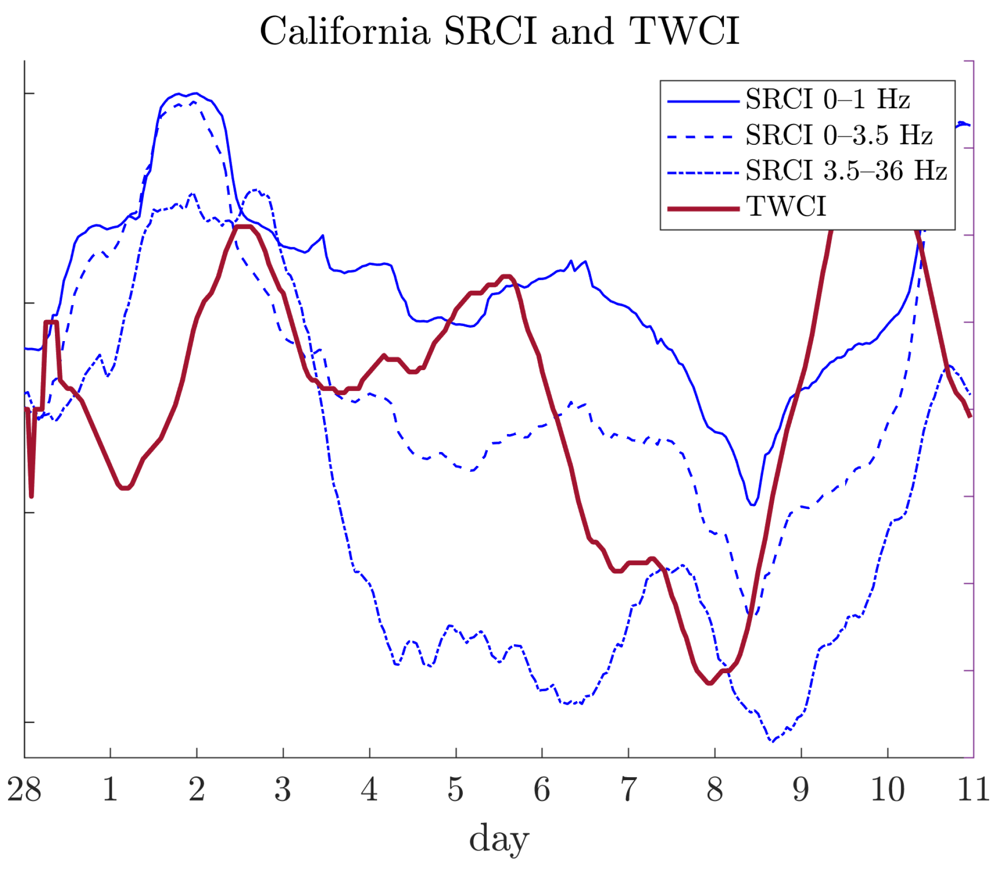
San Francisco, CA, the USA (37.80700, −122.46500)	California (37.4192, −122.057)

). Note that the oceanic water movements do not have a strong impact on the measurement of SRA because all magnetometers of the Global Coherence Monitoring System are located far from the shoreline. An example of the computed results is shown in Figure 12. Note that there is an observable phase difference between the SRCI and TWCI signals in Figure 12. However, we use statistical formulae, not visual comparisons, between plotted signals to derive correlations between signals. The explanation of this phase difference in Figure 12 goes beyond the objectives of this study.

As defined in the previous section, magnetic field data are represented by the SRCI index. To maintain consistency in the comparison between magnetic field and tidal wave data, we introduce the Tidal Wave Complexity Index (TWCI). The computation methodology for the TWCI remains the same as that presented for the SRCI in previous sections.

The size of the Hankel matrix used to embed the tidal wave data is set to 24 × 24 due to the hourly sea level measurements. H-rank computations are performed in overlapping observation windows (the width of the window is set to 48 data points). Computations continue until the last data point in the two-week observation period is reached. Note that the calibration of $\epsilon$ is performed once for the first 48 iterations. The strategy for the calibration of the threshold parameter $\epsilon$ remains the same as for the SRCI. The aim is to choose such a value of $\epsilon$ that the average TWCI would be exactly equal to 50%. The calibrated threshold parameter $\epsilon$ for each location of the tidal wave is presented in

Table 8. Calibrated threshold parameter $\epsilon$ for TWCI.

Location of the Tidal Waves Measurement Station	Threshold Parameter $\mathit{\epsilon }$
Hanimaadhoo, Maldives	27.2
Dzaoudzi, France	52.9
Honningsvag, Norway	40.5
Easter Island, Chile	147.5
San Francisco, CA, USA	79.5

.

Then, the complexity index characterizing the algebraic complexity of the investigated time series is computed as the arithmetic average of all H-ranks computed on the current day (which automatically eliminates the diel cycle). As previously, the threshold $\epsilon$ is not recalibrated for the subsequent days. Those complexity index values are named as the Tidal Wave Complexity Index (TWCI).

An example of the computed SRCI and TWCI is shown in Figure 12.

5.2. Statistical Analysis

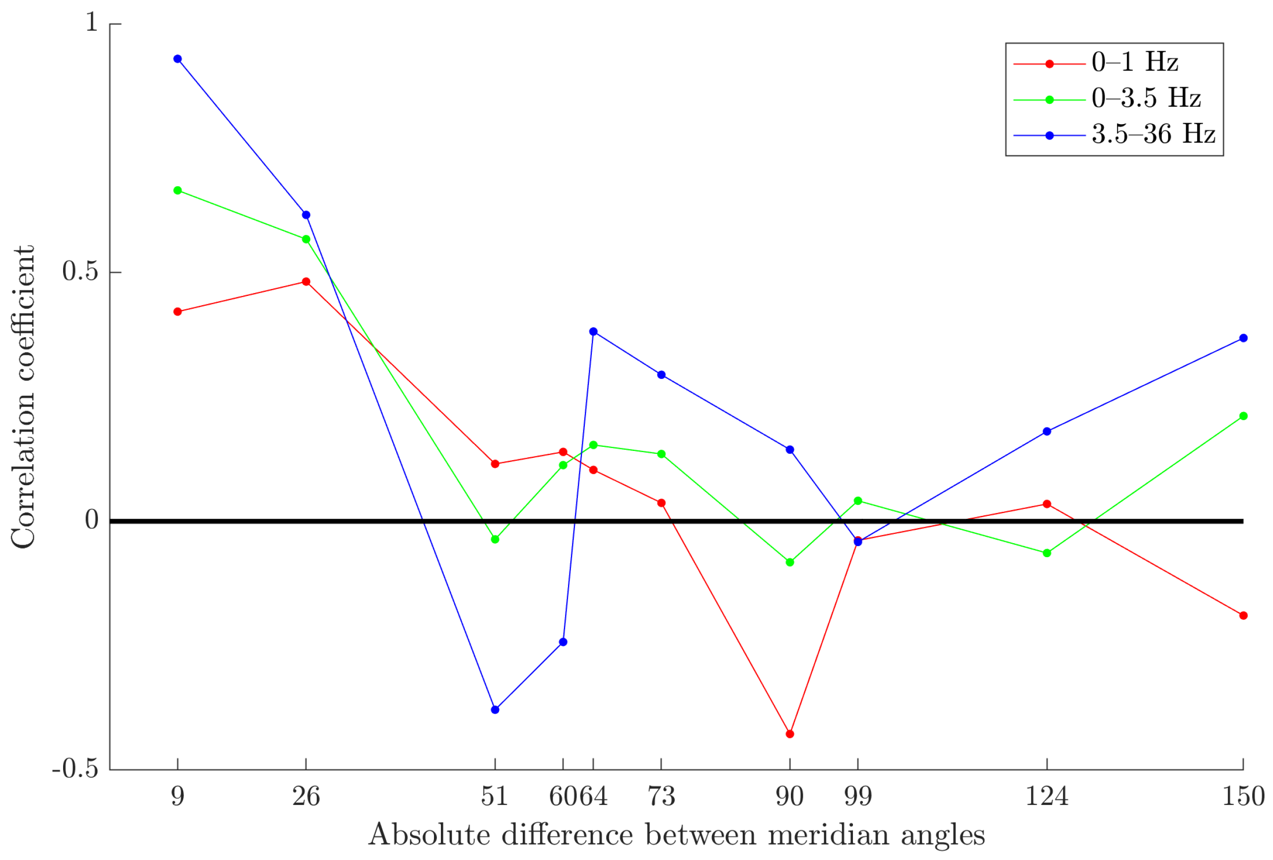
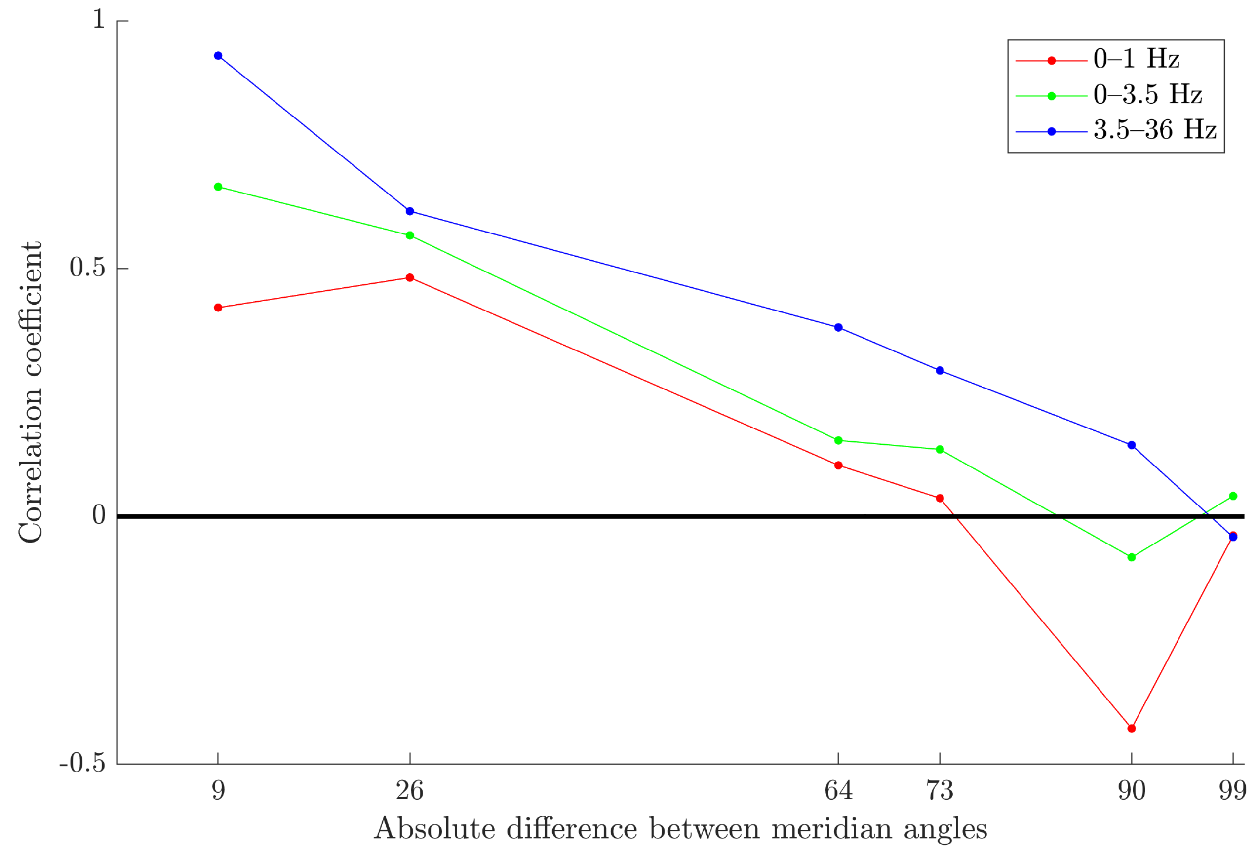
A statistical analysis is performed to confirm or deny the proposed hypothesis that the correlation between local magnetic fields (with the eliminated diel cycle) measured at different locations around the world depends on the absolute difference between the meridian coordinates of those locations (Hypothesis 1) and that the SRCI correlates with the TWCI (Hypothesis 2).

We define the following statistical variables: $X_{i,1}$—SRCI of the ith region in the 0–1 Hz range, $X_{i,2}$—SRCI of the ith region in the 0–3.5 Hz range, $X_{i,3}$—SRCI of the ith region in the 3.5–36 Hz range, $X_{i,4}$—TWCI of the ith region.

Pearson’s linear correlation and Spearman’s rank correlation coefficients are commonly used in the study of the correlation relationship in statistics. Pearson’s coefficient is applied when the data are normal. If the condition of normality of the variables is not satisfied or the data are sparse, Spearman’s rank coefficient is applied.

We check whether the normality condition is satisfied. Applying the chi-square test with a significance level of $\alpha =0.05$, we test the following hypotheses:

$$\begin{array}{cc}\hfill & H_0:X_{i,j}\sim N({\widehat{\mu }}_{i,j},{\widehat{\sigma }}_{i,j}),\hfill \\ \hfill & H_a:X_{i,j}\nsim N({\widehat{\mu }}_{i,j},{\widehat{\sigma }}_{i,j})\hfill \end{array}$$

(6)

here ${\widehat{\mu }}_{i,j},{\widehat{\sigma }}_{i,j}$$(i\in \{1,2,3,4,5\},j\in \{1,2,3,4\left\}\right)$ —parameter estimates found by the maximum likelihood method.

Since in all cases the p-value is lower than the selected level of significance (

Table 9. The results of normality tests.

Region	i	Distribution Parameter Estimation			p-Value ≤
		j	${\widehat{\mathit{\mu }}}_{\mathit{i},\mathit{j}}$	${\widehat{\mathit{\sigma }}}_{\mathit{i},\mathit{j}}$
California	1	1	74.36	10.54	$1.8·{10}^{-8}$
		2	63.77	14.77	$1.1·{10}^{-16}$
		3	48.39	20	0
		4	12.23	1.55	$4.6·{10}^{-4}$
Canada	2	1	58.95	14.34	$1.4·{10}^{-7}$
		2	53.63	14.79	$6.7·{10}^{-4}$
		3	59.48	15.81	0
		4	11.82	3.04	$2.4·{10}^{-14}$
Lithuania	3	1	94.13	2.95	$4.2·{10}^{-3}$
		2	79.36	6.89	$6.3·{10}^{-11}$
		3	76.9	10.31	$3.7·{10}^{-4}$
		4	12.28	1.44	0
Saudi Arabia	4	1	73.96	6.97	0
		2	78.51	7.4	$4·{10}^{-9}$
		3	72.82	9.68	$9·{10}^{-4}$
		4	12.21	1.34	0
New Zealand	5	1	71.12	17.07	$3.6·{10}^{-4}$
		2	85.09	16.4	$3.1·{10}^{-5}$
		3	88.88	14.57	$6.5·{10}^{-8}$
		4	12.07	1.16	$8.6·{10}^{-8}$

), the hypotheses of the normality of variables $X_{i,1},X_{i,2},X_{i,3},X_{i,4},i\in \{1,2,3,4,5\}$ are rejected.

As the normality condition is not satisfied, we will apply Spearman’s rank correlation coefficient. Suppose we have pairs of variables $(X_{i,m},X_{i,s}),i\in \{1,2,3,4,5\},m,s\in \{1,2,3,4\}$ and observations $(X_{i,m}^1,X_{i,s}^1),(X_{i,m}^2,X_{i,s}^2),\cdots ,(X_{i,m}^n,X_{i,s}^n)$. We arrange the observations $X_{i,m}^1,X_{i,m}^2,\cdots ,X_{i,m}^n$ and $X_{i,s}^1,X_{i,s}^2,\cdots ,X_{i,s}^n$ separately. Let $R\left(X_{i,t}^k\right)$ be the rank of observation $X_{i,t}^k$. Then, the Spearman’s rank correlation coefficient is given by

$$r_{m,s}^i=\frac{{\displaystyle \sum _{k=1}^n}(R\left(X_{i,m}^k\right)-\frac{n+1}{2})(R\left(X_{i,s}^k\right)-\frac{n+1}{2})}{\sqrt{{\displaystyle \sum _{k=1}^n}{(R\left(X_{i,m}^k\right)-\frac{n+1}{2})}^2}\sqrt{{\displaystyle \sum _{k=1}^n}{(R\left(X_{i,s}^k\right)-\frac{n+1}{2})}^2}}$$

(7)

We calculate the Spearman’s correlation coefficient between the variables in each region (

Table 10. Spearman’s correlation coefficient values ($i=1$, region—California).

$r_{m,s}^i$	$X_{i,1}$	$X_{i,2}$	$X_{i,3}$	$X_{i,4}$
$X_{i,1}$	1	0.95	0.72	0.22
$X_{i,2}$	0.95	1	0.82	0.18
$X_{i,3}$	0.72	0.82	1	0.25
$X_{i,4}$	0.22	0.18	0.25	1

represents the Spearman’s correlation coefficients in California,

Table 11. Spearman’s correlation coefficient values ($i=2$, region—Canada).

$r_{m,s}^i$	$X_{i,1}$	$X_{i,2}$	$X_{i,3}$	$X_{i,4}$
$X_{i,1}$	1	0.89	0.45	0.45
$X_{i,2}$	0.89	1	0.70	0.22
$X_{i,3}$	0.45	0.70	1	−0.23
$X_{i,4}$	0.45	0.22	−0.23	1

the coefficients in Canada,

Table 12. Spearman’s correlation coefficient values ($i=3$, region—Lithuania).

$r_{m,s}^i$	$X_{i,1}$	$X_{i,2}$	$X_{i,3}$	$X_{i,4}$
$X_{i,1}$	1	0.94	0.88	0.31
$X_{i,2}$	0.94	1	0.89	0.43
$X_{i,3}$	0.88	0.89	1	0.41
$X_{i,4}$	0.31	0.43	0.41	1

those in Lithuania,

Table 13. Spearman’s correlation coefficient values ($i=4$, region—Saudi Arabia).

$r_{m,s}^i$	$X_{i,1}$	$X_{i,2}$	$X_{i,3}$	$X_{i,4}$
$X_{i,1}$	1	0.92	0.80	0.14
$X_{i,2}$	0.92	1	0.90	0.26
$X_{i,3}$	0.80	0.90	1	0.28
$X_{i,4}$	0.14	0.26	0.28	1

those in Saudi Arabia, and

Table 14. Spearman’s correlation coefficient values ($i=5$, region—New Zealand).

$r_{m,s}^i$	$X_{i,1}$	$X_{i,2}$	$X_{i,3}$	$X_{i,4}$
$X_{i,1}$	1	0.96	0.72	−0.05
$X_{i,2}$	0.96	1	0.86	0.04
$X_{i,3}$	0.72	0.86	1	0.24
$X_{i,4}$	−0.05	0.04	0.24	1

the coefficients in New Zealand).

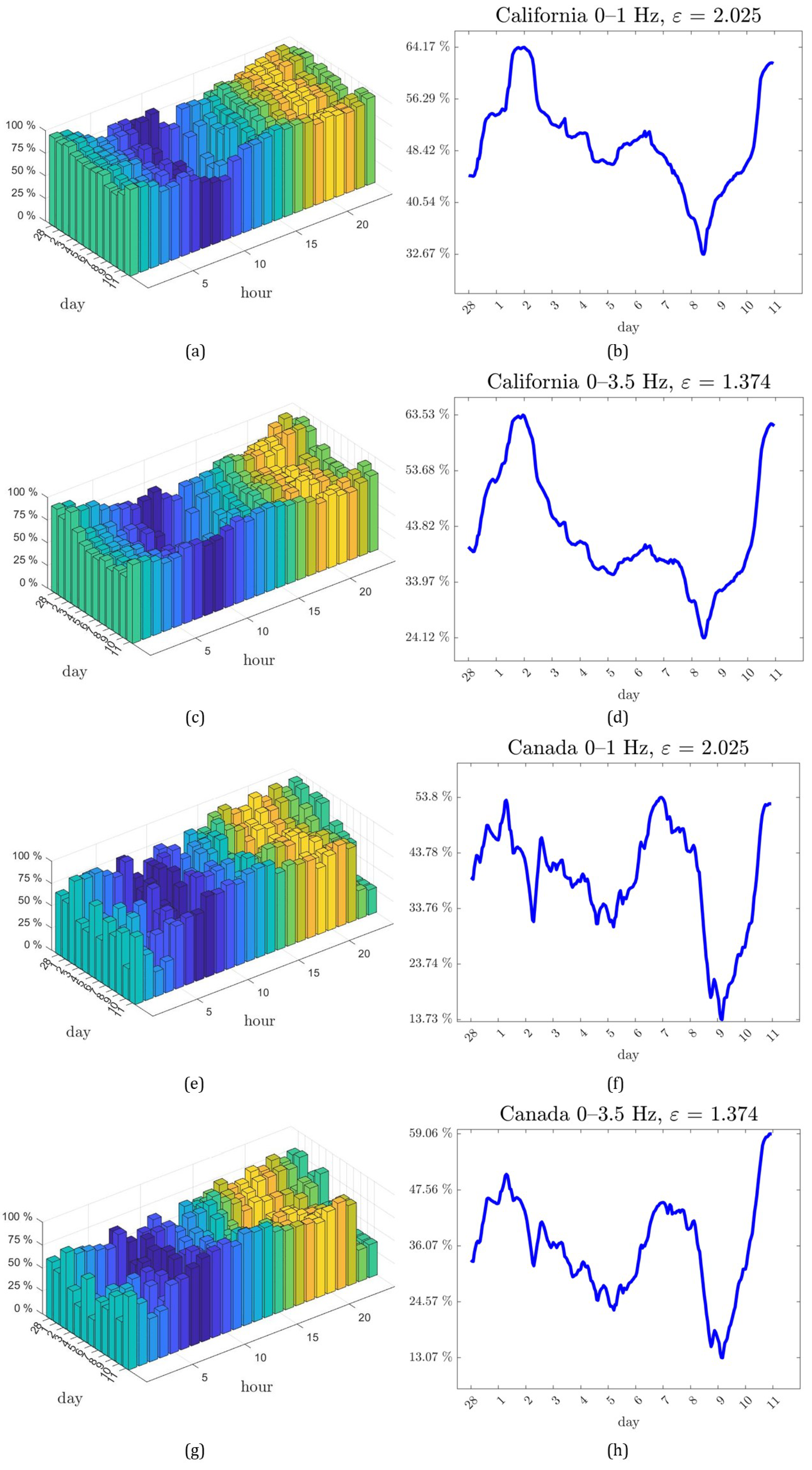
The results obtained suggest that the correlation between pairs of variables $X_{i,1},X_{i,2},X_{i,3},i\in \{1,2,3,4,5\}$, in each region is strong or very strong, with the exception of the Canadian region, where the pair $(X_{2,1},X_{2,3})$ exhibits a moderate strength of connection. However, it should be noted that in each region between variables $X_{i,1},X_{i,2},X_{i,3}$ and variable $X_{i,4},i\in \{1,2,3,4,5\}$ there is a very weak or non-existent relationship.

To determine the statistical significance of the values of the correlation coefficients obtained, we subject the results to hypothesis testing. We test the following hypotheses:

$$\begin{array}{cc}\hfill & H_0:r_{m,s}^i=0,\hfill \\ \hfill & H_a:r_{m,s}^i\ne 0\hfill \end{array}$$

(8)

where $i\in \{1,2,3,4,5\},m\ne s,(m,s)\in \{1,2,3,4\}$.

The following statistical measure is used to test the hypothesis:

$$T_{m,s}^i=r_{m,s}^i\sqrt{\frac{n-2}{1-{\left(r_{m,s}^i\right)}^2}}$$

(9)

When the null hypothesis $H_0$ is true, the distribution of the statistic $T_{m,s}^i$ follows a Student’s t-distribution with $(n-2)$ degrees of freedom. Therefore, the p-value for the applied criterion is calculated as follows:

$$P_{m,s}^i=P\left(\right|T|\ge |T_{m,s}^i\left|\right)$$

(10)

where T is a random variable distributed according to the Student’s t-distribution with $(n-2)$ degrees of freedom.

We select the significance level $\alpha =0.05$ to evaluate each hypothesis. The p-value for each hypothesis is then calculated. If the p-value is less than or equal to $\alpha =0.05$ we reject the null hypothesis, indicating a statistically significant result. Conversely, if the p-value is greater than $\alpha =0.05$, we fail to reject the null hypothesis, suggesting a lack of statistical significance.

Table 15. The results of testing of significance of the correlation coefficients.

Region	i	${\mathbf{P}}_{1,2}^{\mathbf{i}}$	${\mathbf{P}}_{1,3}^{\mathbf{i}}$	${\mathbf{P}}_{1,4}^{\mathbf{i}}$	${\mathbf{P}}_{2,3}^{\mathbf{i}}$	${\mathbf{P}}_{2,4}^{\mathbf{i}}$	${\mathbf{P}}_{3,4}^{\mathbf{i}}$
California	1	0	0	$4·{10}^{-8}$	0	$8.2·{10}^{-5}$	$4·{10}^{-5}$
Canada	2	0	$1.4·{10}^{-14}$	$6.3·{10}^{-14}$	0	$1.6·{10}^{-4}$	$4·{10}^{-5}$
Lithuania	3	0	0	$5.1·{10}^{-11}$	0	0	$6.7·{10}^{-16}$
Saudi Arabia	4	0	0	$3.3·{10}^{-3}$	0	$6.8·{10}^{-7}$	$1.6·{10}^{-6}$
New Zealand	5	0	0	$4.2·{10}^{-1}$	0	$4.2·{10}^{-1}$	$3.2·{10}^{-4}$

indicates that, for the regions of the USA, Canada, Lithuania, and Saudi Arabia, the Spearman’s rank correlation coefficients are significantly different from zero. This implies that the null hypotheses $H_0$, which assert that the quantities are not correlated, are rejected in these cases. In the case of New Zealand, it should be noted that the hypotheses of the non-correlation between the quantities $X_{5,1}$ and $X_{5,4}$, $X_{5,2}$ and $X_{5,4}$ cannot be rejected. This outcome is likely due to the fact that the values of the Spearman’s rank correlation coefficient are close to 0.

6. Concluding Remarks

As a result of the research presented in this article, we introduced the Schumann Resonance Complexity Index (SRCI). This is a new complexity measure designed for the measurement of algebraic complexity in magnetometers within the Global Coherence Network. This result is particularly interesting, as it fundamentally differs from all other measures of magnetic field complexity, such as the Kp index and other indices that globally represent the properties of the Earth’s magnetic field.

On further analysis, we observed that the elimination of diel cycles from the SRCI data yields interesting results. It appears that the correlations between different magnetometers are strongly related to the meridian angles: the smaller the difference in absolute values between the meridian angles, the larger the correlation between different magnetometers. No such similarities would be noticed when analyzing the raw magnetic field signals alone. This is the second result of this article, allowing the exploration of connections between different magnetometers.

This similarity immediately gives rise to a series of hypotheses. The first hypothesis suggests that if meridians play a significant role in the similarity between different magnetometers, it should be related to the influence of the Moon. However, since the magnetic field is measured locally at specific geographic locations, our intention was to evaluate the local tidal effects caused by the Moon. Fortunately, the existence of the global network of tidal waves (significantly larger than the global network of magnetometers) makes this task possible. The selection of the tidal wave monitoring station for each individual magnetometer was based on proximity. However, the geographical proximity was not the only important factor—the meridian proximity was taken into consideration because of the raised hypothesis.

Note that we did not directly measure correlations between the SRCI data and the tidal wave data. In principle, the signals are entirely different: the sampling rate of the magnetic field is 130 Hz, whereas tidal waves constitute one measurement per hour. Despite this, we introduce an identical complexity measure for tidal waves: the Tidal Wave Complexity Index (TWCI).

Having two indices, the Schumann Resonance Complexity Index (SRCI) and the Tidal Wave Complexity Index (TWCI), makes it possible to statistically and reliably explore possible connections. The statistical analysis yields truly intriguing results. And though the New Zealand magnetometer falls out of the rule, all the remaining magnetometers appear to be significantly correlated to the tidal effects. Thus, the main result of this article is the demonstration of the fact that the influence of the Moon (usually observed through tidal waves) affects the readings of the local magnetic field data recorded by the global network of magnetometers. Although this is the first demonstration of such an effect, in principle it is not astonishing. It is well known that tidal effects induced by the Moon affect not only water tides but also crustal displacements and the magnetosphere of the Earth. Naturally, one could expect that the same effects will also manifest in the local magnetic field. This study confirms this fact.

7. Discussion and Limitations

Possibly, the elimination of the diel cycle removes not only Sq variations (over a 24 h period) from the magnetic data, but also some part of the 12 h interval, which is close to the period of the lunar tidal wave. Therefore, emphasizing the lunar effect in magnetic variations is very difficult.

The five magnetic stations are located across the Earth, starting from Alberta, Northern Canada, to Baisiogala, Lithuania, Eastern Europe, close to subauroral latitudes. In this case, latitudinal and longitudinal magnetic variations due to lunar tidal waves can also be discussed.

There are several studies exploring the varying influences of high-latitude electric fields and atmospheric waves on daily fluctuations of ionospheric currents [49], studying the seasonal longitudinal climatology of semi-diurnal lunar tidal variation in the equatorial electrojet [50], describing the semi-diurnal lunar tidal influence on neutral winds, plasma velocities, and atomic oxygen airglow [51], and exploring semi-diurnal tidal variations and their effects on the ionosphere–thermosphere–mesosphere system [52].

This work focuses exclusively on the coordinates of the meridian and delves into the essence of tidal waves. Although other aspects, such as different coordinates and types of waves, could be explored, they remain beyond the scope of this study. These areas could serve as subjects for future research efforts, extending the understanding of tidal phenomena and local magnetic field in diverse contexts.

It is well established that the Moon influences the global and local magnetic field of the Earth, a fact confirmed and demonstrated through detailed studies performed not with data from five magnetometers scattered around the world but with data from dozens of magnetometers belonging to regular (and officially recognized by the scientific community) geomagnetic observatories covering our planet in latitude and longitude. Although the results discussed herein are based on the analysis of limited data over time and from few observation sites, the statistical treatment of the presented data is undoubtedly correct and appropriate. Geomagnetic conditions were not considered or characterized in this study, but could be a topic for further research.

An area for potential improvement in the study lies in the comparison of data between local magnetic field measurement sites and nearby tidal wave measurement stations, rather than prioritizing comparison based on geomagnetic proximity. It should be noted that the global dipolar magnetic field establishes geomagnetic coordinates, a crucial reference system for understanding conjugate effects between distinct points on Earth’s surface.

References

1. Bartels, J. The standardized index, Ks, and the planetary index, Kp. IATME Bull. 1949, 97–120. [Google Scholar]
2. Matzka, J.; Stolle, C.; Yamazaki, Y.; Bronkalla, O.; Morschhauser, A. The Geomagnetic Kp Index and Derived Indices of Geomagnetic Activity. Space Weather 2021, 19, e2020SW002641. [Google Scholar] [CrossRef]
3. Sugiura, M. Hourly values of equatorial Dst for the IGY. Ann. Int. Geophys. Year 1964, 35. [Google Scholar]
4. Johnson, E.A.; Murphy, T.; Torreson, O.W. Pre-history of the Earth’s magnetic field. Terr. Magn. Atmos. Electr. 1948, 53, 349–372. [Google Scholar] [CrossRef]
5. Friis-Christensen, E.; Lühr, H.; Hulot, G. Swarm: A constellation to study the Earth’s magnetic field. Earth Planets Space 2006, 58, 351–358. [Google Scholar] [CrossRef]
6. Introduction to Geomagnetism. Available online: https://www.usgs.gov/programs/geomagnetism/introduction-geomagnetism (accessed on 7 August 2023).
7. Methods and Apparatus for Magnetic Field Shimming. Available online: https://patents.google.com/patent/US10788550B2/en (accessed on 7 August 2023).
8. World Magnetic Model (WMM). Available online: https://www.ncei.noaa.gov/products/world-magnetic-model (accessed on 7 August 2023).
9. Smith, C.; L’Heureux, J.; Ness, N.; Acuña, M.; Burlaga, L.; Scheifele, J. The ACE Magnetic Fields Experiment. Space Sci. Rev. 1998, 86, 613–632. [Google Scholar] [CrossRef]
10. Mandea, M.; Purucker, M. The Varying Core Magnetic Field from a Space Weather Perspective. Space Sci. Rev. 2017, 214, 11. [Google Scholar] [CrossRef]
11. Tsyganenko, N.A. Empirical Magnetic Field Models for the Space Weather Program. Space Weather 2001, 125, 273–280. [Google Scholar] [CrossRef]
12. Popova, E.; Popov, A.I.; Sagdeev, R. Multimode Representation of the Magnetic Field for the Analysis of the Nonlinear Behavior of Solar Activity as a Driver of Space Weather. Mathematics 2022, 10, 1655. [Google Scholar] [CrossRef]
13. Singer, H.; Matheson, L.; Grubb, R.; Newman, A.; Bouwer, D. Monitoring space weather with the GOES magnetometers. In Proceedings of the GOES-8 and Beyond, Denver, CO, USA, 4–9 August 1996; Washwell, E.R., Ed.; International Society for Optics and Photonics, SPIE: Bellingham, WA, USA, 1996; Volume 2812, pp. 299–308. [Google Scholar] [CrossRef]
14. Mandea, M.; Chambodut, A. Geomagnetic Field Processes and Their Implications for Space Weather. Surv. Geophys. 2020, 41, 1611–1627. [Google Scholar] [CrossRef]
15. Ringler, A.T.; Anthony, R.E.; Wilson, D.C.; Claycomb, A.C.; Spritzer, J. Magnetic Field Variations in Alaska: Recording Space Weather Events on Seismic Stations in Alaska. Bull. Seismol. Soc. Am. 2020, 110, 2530–2540. [Google Scholar] [CrossRef]
16. Welling, D.T.; Ridley, A.J. Validation of SWMF magnetic field and plasma. Space Weather 2010, 8, 2530–2540. [Google Scholar] [CrossRef]
17. Heart Math GCMS. Available online: https://www.heartmath.org/gci/gcms/ (accessed on 7 August 2023).
18. Jan, G.; Gómez, B.P.; Salaün, C.; Rouxel, D.; Pouvreau, N.; Ferret, Y.; Latapy, A. Measurement for the Sea: Supporting the Marine Environment and the Blue Economy; Springer International Publishing: Cham, Switzerland, 2022; pp. 237–270. [Google Scholar] [CrossRef]
19. Tolkatchev, A. Global sea level observing system (GLOSS). Mar. Geod. 1996, 19, 21–62. [Google Scholar] [CrossRef]
20. Xiao, C.; He, F.; Shi, Q.e.a. Evidence for lunar tide effects in Earth’s plasmasphere. Nat. Phys. 2023, 19, 486–491. [Google Scholar] [CrossRef]
21. McCraty, R.; Deyhle, A. The global coherence initiative: Investigating the dynamic relationship between people and earth’s energetic systems. Bioelectromagn. Subtle Energy Med. 2015, 2, 411–425. [Google Scholar] [CrossRef]
22. Timofejeva, I.; McCraty, R.; Atkinson, M.; Alabdulgader, A.A.; Vainoras, A.; Landauskas, M.; Šiaučiūnaitė, V.; Ragulskis, M. Global Study of Human Heart Rhythm Synchronization with the Earth’s Time Varying Magnetic Field. Appl. Sci. 2021, 11, 2935. [Google Scholar] [CrossRef]
23. Kuzmin, A.; Nechaev, A.; Kurakin, A.A. Linear complexity of polinear sequences. J. Math. Sci. 1995, 76, 2793–2915. [Google Scholar]
24. Ragulskis, M.; Navickas, Z. The rank of a sequence as an indicator of chaos in discrete nonlinear dynamical systems. Commun. Nonlinear Sci. Numer. Simul. 2011, 16, 2894–2906. [Google Scholar] [CrossRef]
25. Klema, V.; Laub, A. The singular value decomposition: Its computation and some applications. IEEE Trans. Autom. Control 1980, 25, 164–176. [Google Scholar] [CrossRef]
26. Boccaletti, S.; Valladares, D.L. Characterization of intermittent lag synchronization. Phys. Rev. E 2000, 62, 7497–7500. [Google Scholar] [CrossRef]
27. Brown, R.; Rulkov, N.F.; Tracy, E.R. Modeling and synchronizing chaotic systems from time-series data. Phys. Rev. E 1994, 49, 3784–3800. [Google Scholar] [CrossRef]
28. Tang, Y.; Qian, F.; Gao, H.; Kurths, J. Synchronization in complex networks and its application—A survey of recent advances and challenges. Annu. Rev. Control 2014, 38, 184–198. [Google Scholar] [CrossRef]
29. Huygens, C. Instructions concerning the use of pendulum-watches, for finding the longitude at sea. Philos. Trans. R. Soc. Lond. 1997, 4, 937–953. [Google Scholar] [CrossRef]
30. Pecora, L.M.; Carroll, T.L. Synchronization in chaotic systems. Phys. Rev. Lett. 1990, 64, 821–824. [Google Scholar] [CrossRef]
31. Carroll, T.L.; Pecora, L.M. Synchronizing nonautonomous chaotic circuits. IEEE Trans. Circuits Syst. II Analog Digit. Signal Process. 1993, 40, 646–650. [Google Scholar] [CrossRef]
32. Kocarev, L.; Parlitz, U. General Approach for Chaotic Synchronization with Applications to Communication. Phys. Rev. Lett. 1995, 74, 5028–5031. [Google Scholar] [CrossRef]
33. Koronovskii, A.A.; Moskalenko, O.I.; Hramov, A.E. On the use of chaotic synchronization for secure communication. Phys.-Uspekhi 2009, 52, 1213. [Google Scholar] [CrossRef]
34. Reidler, I.; Nixon, M.; Aviad, Y.; Guberman, S.; Friesem, A.A.; Rosenbluh, M.; Davidson, N.; Kanter, I. Coupled lasers: Phase versus chaos synchronization. Opt. Lett. 2013, 38, 4174–4177. [Google Scholar] [CrossRef]
35. Uchida, A.; Rogister, F.; García-Ojalvo, J.; Roy, R. Synchronization and communication with chaotic laser systems. Prog. Opt. 2005, 48, 203–341. [Google Scholar] [CrossRef]
36. Uhlhaas, P.J.; Singer, W. Neural Synchrony in Brain Disorders: Relevance for Cognitive Dysfunctions and Pathophysiology. Neuron 2006, 52, 155–168. [Google Scholar] [CrossRef]
37. Li, Y.N.; Chen, L.; Cai, Z.S.; Zhao, X.Z. Experimental study of chaos synchronization in the Belousov–Zhabotinsky chemical system. Chaos Solitons Fractals 2004, 22, 767–771. [Google Scholar] [CrossRef]
38. Rohden, M.; Sorge, A.; Timme, M.; Witthaut, D. Self-Organized Synchronization in Decentralized Power Grids. Phys. Rev. Lett. 2012, 109, 064101. [Google Scholar] [CrossRef]
39. Wang, P.; Wen, G.; Yu, X.; Yu, W.; Huang, T. Synchronization of Multi-Layer Networks: From Node-to-Node Synchronization to Complete Synchronization. IEEE Trans. Circuits Syst. I Regul. Pap. 2019, 66, 1141–1152. [Google Scholar] [CrossRef]
40. Ahmadlou, M.; Adeli, H. Visibility graph similarity: A new measure of generalized synchronization in coupled dynamic systems. Phys. D Nonlinear Phenom. 2012, 241, 326–332. [Google Scholar] [CrossRef]
41. Hoon, Y.; Mohd Radzi, M.A.; Mohd Zainuri, M.A.A.; Zawawi, M.A.M. Shunt Active Power Filter: A Review on Phase Synchronization Control Techniques. Electronics 2019, 8, 791. [Google Scholar] [CrossRef]
42. Gonzalez-Miranda, J.M. Amplitude envelope synchronization in coupled chaotic oscillators. Phys. Rev. E 2002, 65, 036232. [Google Scholar] [CrossRef]
43. Sun, W.; Wang, S.; Wang, G.; Wu, Y. Lag synchronization via pinning control between two coupled networks. Nonlinear Dyn. 2015, 79, 2659–2666. [Google Scholar] [CrossRef]
44. Ciszak, M.; Mayol, C.; Mirasso, C.R.; Toral, R. Anticipated synchronization in coupled complex Ginzburg-Landau systems. Phys. Rev. E 2015, 92, 032911. [Google Scholar] [CrossRef]
45. May, R.M. Simple mathematical models with very complicated dynamics. Nature 1976, 261, 459–467. [Google Scholar] [CrossRef]
46. Alabdulgader, A.; McCraty, R.; Atkinson, M.; Dobyns, Y.; Vainoras, A.; Ragulskis, M.; Stolc, V. Long-Term Study of Heart Rate Variability Responses to Changes in the Solar and Geomagnetic Environment. Sci. Rep. 2018, 8, 2663. [Google Scholar] [CrossRef]
47. Sátori, G.; Neska, M.; Williams, E.; Szendrői, J. Signatures of the day-night asymmetry of the Earth-ionosphere cavity in high time resolution Schumann resonance records. Radio Sci. 2007, 42, 1–16. [Google Scholar] [CrossRef]
48. University of Hawaii. Sea Level Centre. Available online: https://uhslc.soest.hawaii.edu/data/ (accessed on 7 August 2023).
49. Yamazaki, Y.; Häusler, K.; Wild, J.A. Day-to-day variability of midlatitude ionospheric currents due to magnetospheric and lower atmospheric forcing. J. Geophys. Res. Space Phys. 2016, 121, 7067–7086. [Google Scholar] [CrossRef]
50. Yamazaki, Y.; Stolle, C.; Matzka, J.; Siddiqui, T.A.; Lühr, H.; Alken, P. Longitudinal Variation of the Lunar Tide in the Equatorial Electrojet. J. Geophys. Res. Space Phys. 2017, 122, 12445–12463. [Google Scholar] [CrossRef]
51. Lieberman, R.S.; Harding, B.J.; Heelis, R.A.; Pedatella, N.M.; Forbes, J.M.; Oberheide, J. Atmospheric Lunar Tide in the Low Latitude Thermosphere-Ionosphere. Geophys. Res. Lett. 2022, 49, e2022GL098078. [Google Scholar] [CrossRef]
52. Goncharenko, L.; Liu, H.L.; Chau, J.; Stober, G.; Sunkara, E.; Zabotin, N. Importance of the semidiurnal tide, and future measurements needed to improve its characterization. Bull. Am. Astron. Soc. 2023, 55. [Google Scholar] [CrossRef]
Figure 1. MSC logistic map at Δ = 0.1 in panel (a) and σ 2 in panel (b).
Applsci 14 03332 g001
Figure 2. MSC logistic map at Δ = 0.5 in panel (a) and σ 2 in panel (b).
Applsci 14 03332 g002
Figure 3. The schematic explanation of the H-rank computations for the time series.
Applsci 14 03332 g003
Figure 4. Twenty-four complexity indices computed for the MSC logistic maps (the difference time series x k y k ). The parameters of the H-rank algorithm are set to d = 150 and ε = 0.15. The coupling parameter Δ is set to 0.1 in panel (a); 0.3 in panel (b); 0.4 in panel (c); 0.425 in panel (d); 0.45 in panel (e); and 0.5 in panel (f). The left vertical axis and the light gray line stand for the time series x k y k . The red vertical axis and the thin red line stand for the H-ranks computed in overlapping observation windows. Blue bars stand for the complexity indices (the magnitude of the complexity indices is measured by the same scale used to measure unsmoothed H-ranks).
Applsci 14 03332 g004
Figure 5. The variation in the magnetic field spectral power recorded by the magnetometer at California on the 28 February 2015 (over a 24 h period) is depicted in panel (a), while panel (b) shows the first 300 s of this recording.
Applsci 14 03332 g005
Figure 6. The H-rank of the magnetic field spectral power and the Schumann Resonance Complexity Index (SRCI), computed with ε = 0.4 for the magnetometer located in California on 28 February 2015, in the frequency range 3.5–36 Hz in panel (a). The average SRCI is represented by the solid black horizontal line, equal to 60.91% in panel (b).
Applsci 14 03332 g006
Figure 7. The H-rank of the magnetic field spectral power and the Schumann Resonance Complexity Index (SRCI), computed with ε = 0.7 for the magnetometer located in California on 28 February 2015, in the frequency range 3.5–36 Hz in panel (a). The average SRCI is represented by the solid black horizontal line, equal to 37.43% in panel (b).
Applsci 14 03332 g007
Figure 8. The calibration of the ε value for the Schumann Resonance Complexity Index (SRCI). Schumann resonance time series recorded by the Californian magnetometer in the frequency range 3.5–36 Hz on 28 February 2015.
Applsci 14 03332 g008
Figure 9. SRCIs computed for the California site in the frequency range 0–1 Hz. The dynamics of the SRCI in the time period between 28 February and 11 March 2015, is shown in panel (a). The color scheme in panel (a) represents the local time (the bright yellow denotes the middle of the day and the dark blue shows the middle of the night). The time shown on the x-axis in panel (a) corresponds to GMT. Moving averages of SRCI (averages with the diel cycle eliminated) are depicted in panel (b). The dynamics of SRCI computed for the California site in the frequency range 0–3.5 Hz are shown in panel (c) and moving averages of the SRCI are depicted in panel (d). The dynamics of the SRCI computed for the Canada site in the frequency range 0–1 Hz are shown in panel (e) and moving averages of the SRCI are depicted in panel (f). The dynamics of the SRCI computed for the Canada site in the frequency range 0–3.5 Hz are shown in panel (g) and moving averages of the SRCI are depicted in panel (h).
Applsci 14 03332 g009
Figure 10. Relation between Pearson’s correlation coefficient and longitude angles where magnetometers are placed (with NZ).
Applsci 14 03332 g010
Figure 11. Relation between Pearson’s correlation coefficient and longitude angles where magnetometers are placed (without NZ).
Applsci 14 03332 g011
Figure 12. SRCIs computed for the magnetometer data located in California in the frequency ranges 0–1 Hz, 0–3.5 Hz, and 3.5–36 Hz are shown in blue. The TWCI computed for the tidal wave measurement station located in California is shown in red. The dynamics of the SRCI and TWCI are depicted for the time period between 28 February and 11 March 2015.
Applsci 14 03332 g012