1. Introduction
The increasing use of sensors in industries, driven by the rise of intelligent sensor systems in Industry 4.0, represents a significant transformation in production and manufacturing processes. These sensors connect devices and systems, enabling machine-to-machine communication to monitor systems and equipment in industrial facilities. Sensors improve product quality, reduce production costs, and increase operational efficiency by processing data locally and making fast, accurate decisions. Furthermore, the evolution of sensor technologies and their integration with other innovations, such as big data, artificial intelligence, and cloud computing, drives Industry 4.0 towards smarter and more automated production. This paradigm shift in the industry offers promising commercial opportunities as sensors become essential in driving innovation and market competitiveness [
1].
In this scenario, machines and managers face daily challenges related to massive data entry and customization in the manufacturing process. Thus, predictive maintenance is a fundamental approach to anticipating failures through advanced analysis, optimizing process efficiency, and promoting proactive resource management, contributing to operational excellence in manufacturing operations [
2,
3,
4,
5,
6].
The use of advanced techniques to develop prediction models has become crucial to taking advantage of the growing volume of data collected in industries. Machine learning techniques shine in this scenario, using algorithms to examine data in real time and predict output values [
7]. It enables meticulous analysis and empowers strategic decision-making based on extensive data sets, addressing the challenges of variety, speed, and volume of information collected in industries [
2].
Considering this, numerous studies have used artificial intelligence techniques to extract valuable insights, helping to make decisions related to industry machine failures. In [
3], the authors have synthesized the most recent works on predictive maintenance, highlighting that 32 studies used actual data to develop predictive models related to maintenance, while two opted for synthetic data. The analysis reveals that 33% of researchers chose Random Forest (RF), 27% opted for Artificial Neural Networks (ANNs), 25% decided on Support Vector Machines (SVMs), and 13% used K-Means.
Feature selection is a fundamental tool in data analysis, machine learning, and data mining, as it can identify the most relevant features, allowing a deeper understanding of the problem under study and helping data professionals and computer scientists understand which aspects of the data have the most significant impact on the model’s predictions. Furthermore, by highlighting the most important features, it is possible to simplify the model, reducing its complexity and making it more computationally efficient [
2,
3,
4,
5,
8]. This step involves choosing the most relevant or informative dataset characteristics to be used in model construction, improving model performance, and reducing dimensionality, interpretability, and computational savings, among other benefits [
9,
10,
11,
12].
Choosing adequate techniques for feature selection and developing prediction models for machine failure classification are critical points in providing accurate information that assists decision-making processes. Furthermore, these techniques could be applied with the aim of identifying the most useful sensors and providing relevant information for analysis. There are still many other questions underexplored in the literature on automatic identification of industrial machine failures. In this context, this study is guided by the following research questions:
Which feature selection techniques are most used for the machine failure prediction problem?
Which feature selection techniques will provide more accurate models for predicting machine failure?
Which machine learning techniques are most adequate for the machine failure prediction problem?
Can feature selection and machine learning help decision-makers choose the most appropriate sensors for acquiring machine data?
Faced with these questions, the Scopus database was used to research these topics, using the keywords “machine learning”, “predictive maintenance”, “feature selection”, “machine failure classification”, “Random Forest” or “Support Vector Machine” or “Artificial Neural Network”. As a result, 15 scientific articles were found, of which 7 are complete articles, 6 are conference papers, and 2 are conference reviews. Only seven articles have returned when selecting only the “article” document type.
Therefore, this work presents an approach based on machine learning and feature selection techniques to improve the accuracy of the classification of failure machines, aiding predictive maintenance. This work will offer the following contributions:
Employ and compare feature selection techniques to improve the accuracy of failure classification by utilizing the most important features.
Present the most relevant feature selection technique for the failure classification problem.
Test different configurations for the three most used machine learning techniques in the literature, according to [
4], and point out which technique improves the accuracy of failure classification using selected features.
Explore how attribute selection can assist in choosing the most appropriate sensors for acquiring data about machines.
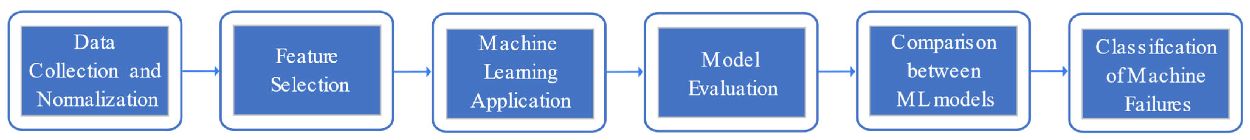
3. Methodology
This section describes the methodology employed to achieve the objectives outlined in this study, covering data collection and normalization, a comparison of four feature selection techniques, the application of three machine learning techniques to develop prediction models, model evaluation and comparison, and the classification of machine failures by using the best model. Detailed descriptions of these steps, illustrated in
Figure 1, are presented below.
3.1. Data Collection and Normalization (Step 1)
This step involves collecting and pre-processing data. First, a dataset related to predictive maintenance, proposed by [
32] and adopted in the study of [
28], was collected from the UC Irvine Machine Learning Repository. This dataset has 10,000 records, each composed of the following attributes: UID, a unique identifier ranging from 1 to 10,000; ProductID, which represents the quality of the product, where L represents 50% of all products, M represents 30% of all products, and H represents 20% of all products; air temperature (K), generated using a random walk process subsequently normalized to a standard deviation of 2 K around 300 K; process temperature (K), generated using a random walk process normalized to a standard deviation of 1 K, added to the air temperature plus 10 K; rotation speed (rpm), calculated from the power of 2860 W, overlaid with customarily distributed noise; torque (Nm) values are typically distributed around 40 Nm with σ = 10 Nm and no negative values; tool wear (min), H/M/L quality variants add 5/3/2 min of tool wear to the tool used in the process; target label indicates whether the machine failed or not at this specific data point; and failure type represents a specific type of failure, including no failure, heat dissipation failure, power failure, random failure, overstrain failure, and tool wear failure.
The data are imbalanced, with a low incidence of some types of failures. There are 9652 no failure samples, 112 heat dissipation failure, 95 power failure samples, 78 overstrain failure samples, 45 tool wear failure samples, and 18 random failure samples.
In the pre-processing procedure, the data were normalized to the interval [0, 1] using the Min-Max approach with the resources of the MinMaxScaler library from Sklearn in Python to avoid differences in the scales of the variables.
Since real predictive maintenance data are often difficult to obtain, this dataset represents an important source of data, because according to [
28,
32], it reflects the real predictive maintenance found in the industry.
3.2. Feature Selection and Comparison of Techniques (Step 2)
This step involves applying and comparing the techniques Principal Component Analysis (PCA), Minimum Redundancy Maximum Relevance (mRMR), Neighborhood Component Analysis (NCA), and Denoising Autoencoder (DAE) to select the best features related to machine failures.
In this work, PCA was applied to the data as indicated by [
19,
20] to verify each variable’s percentage of total variance using the main components. To do this, we employed Sklearn’s PCA Decomposition library in Python, which has a function called explained_variance_ratio. This function calculates the cumulative proportion of the explained variance and returns the total number of principal components with the percentage contribution of each variable to each component. The mRMR was provided by pymrmr library in Python. It receives the input and output variables and returns the relevance level of each input variable about the output. The sklearn.neighbors library was used to provide the correlation levels between the input and output variables using NCA. The procedure involves showcasing input and output variables while partitioning 70% of the data for training and reserving 30% for testing. Finally, the DAE technique was applied using Keras and Tensorflow version 2.15.0. As mentioned before, it is a useful tool to deal with dimensionality reduction and feature selection.
In this study, we employ the technique using TensorFlow’s input, model, and dense libraries.Keras.layers and models. We employ a dense with nine inputs and relu activation function for the encoding layer, while we use the linear activation function for decoding. Furthermore, we applied the Adam optimizer with 100 epochs, a batch size 64, and the mean squared error metric as a loss function. To evaluate the contributions of each variable, we extract the weights from the autoencoder-encoded layer and apply them to the corresponding variables.
Each of these techniques was employed to extract important features from the data and reduce the dimensionality of the feature set. We also sought to observe the level of importance attributed to each resource through these techniques. Subsequently, we compared the best features highlighted by each technique.
It is important to highlight that the RF technique, being based on Decision Trees (DTs), can be used for feature selection by analyzing the contribution of each attribute (variable) to the model’s prediction capability. During the training of the RF algorithm, attributes are evaluated in each individual DT to measure how much each one contributes to reducing impurity in the tree nodes. Then, the importance of each attribute is calculated by the average or sum of impurity reductions across all DTs in the forest. Thus, attributes with greater impurity reductions are considered more important for the model, while those with lesser impact are deemed less relevant and may even be discarded during the DT construction process. Therefore, we also included in the results an analysis of the importance of attributes based on RF.
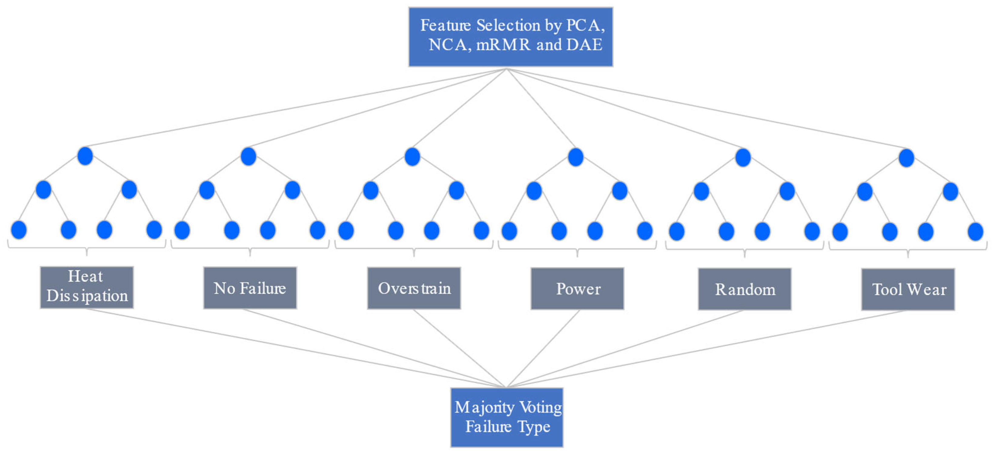
3.3. Failure Classification Using Machine Learning Techniques (Step 3)
Given its effectiveness, as pointed out by researchers in [
33], we developed a Random Forest (RF) model to classify the failure type. RF is a machine learning technique that creates an ensemble of decision trees during training and then makes predictions based on decisions from those trees. For classification, each tree “votes” a class for a specific input [
6,
10,
27,
33].
Figure 2 illustrates the process of RF training, which considers the most important input variables, defined by the feature selection technique, to produce the output indicating the type of failure after each tree votes for one of the six possible failure classes. The model training was conducted with 50, 100, and 200 estimators (trees), separating 70% of the data for training and 30% for testing. We used accuracy, precision, and recall metrics to evaluate the model, as indicated in [
11,
26,
27,
28].
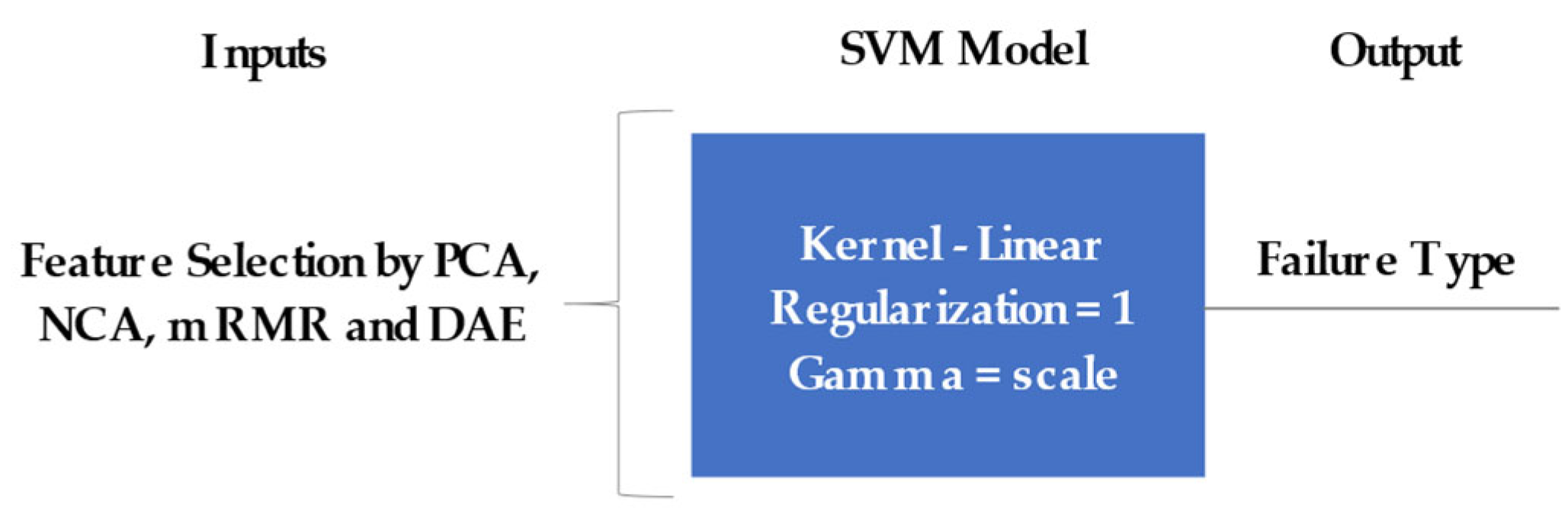
Afterward, the Support Vector Machine (SVM) technique was employed. Its objective is to maximize the margin between different planes. SVM seeks to find a hyperplane that separates instances of different classes in a feature space. A hyperplane is the decision surface that maximizes the margin (support vectors) between opposing class examples [
3,
10,
20].
Figure 3 illustrates the architecture of the SVM model for failure classification, which comprises input, hidden, and output layers. In the hidden layer, the linear kernel functions, regularization equal to 1, and gamma equal to scale were used.
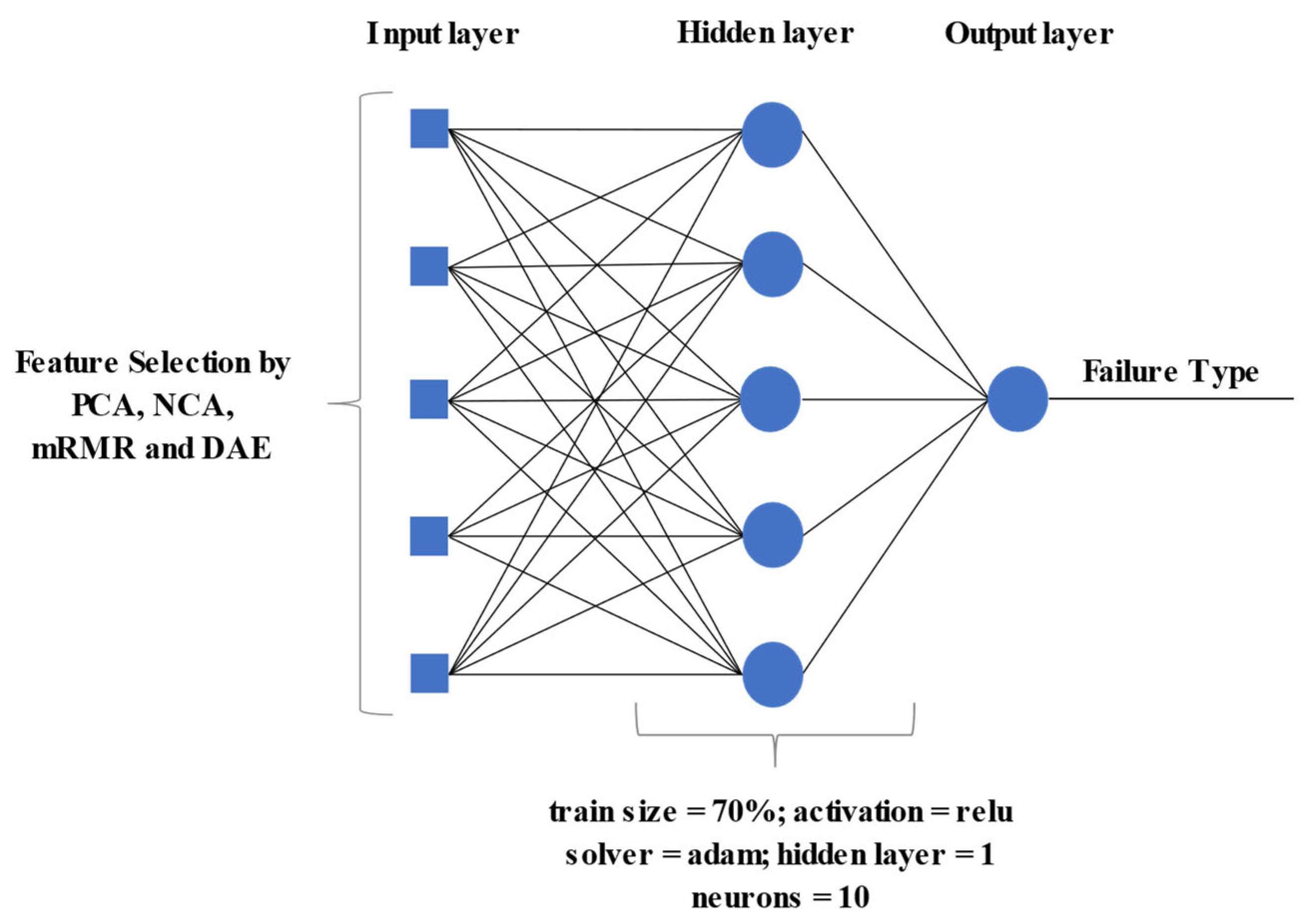
Finally, the Multilayer Perceptron Neural Network (MLP) technique was used to classify machine failures. This sophisticated architecture includes an input layer for data reception, hidden layers for applying non-linear transformations via activation functions, and an output layer for generating predictions. Each neuron connection has a weight, and the output layer’s function depends on the task, which can be sigmoid for binary classification or SoftMax for multiclass classification. The training process involves forward propagation for network output calculation, a loss function for output comparison, and backpropagation for weight and bias adjustment. Optimization algorithms iterate this process to minimize loss [
7,
26,
34].
Figure 4 illustrates the MLP neural network’s architecture used in this research. It comprises three layers: input, hidden, and output. The number of neurons in the hidden layer (
) was determined using the method developed by [
34], described by Equation (1), in which
and
are, respectively, the number of input and output variables.
Additionally, the parameters adopted include the SoftMax activation function and the Adam solver, which are most used in the literature, as indicated by [
34]. The training was conducted with 100 epochs using 70% of the data. The remaining 30% was used for testing.
3.4. Model Evaluation (Step 4)
Accuracy, precision, and recall metrics were utilized to evaluate the performance of RF, SVM, and MLP. The accuracy calculates the proportion of correctly classified instances among the total number of instances in the dataset. Precision is a metric that measures the proportion of correctly predicted positive cases (true positives) among all instances predicted as positive, regardless of whether they were actually positive or negative. The recall metric focuses on the proportion of actual positive cases that are correctly identified by the model and is calculated as the ratio of true positives to the sum of true positives and false negatives [
10,
26].
3.5. Model Comparison (Step 5)
In this step, the three classification models, RF, SVM, and MLP, are compared to determine which machine learning technique offers the best performance in machine failure classification. Performance metrics such as accuracy, precision, and recall are used to analyze each model’s capabilities comprehensively.
Finally, step 6 selects the model that performs best according to these metrics to classify machine failures.
4. Results and Discussions
First, the results are presented by applying feature selection techniques (PCA, mRMR, NCA, and DAE). Then, considering the most relevant features, we evaluate the performance of RF, SVM, and MLP in predicting machine failures in terms of accuracy, precision, and recall. In both cases, feature selection and classification, the results obtained by the techniques are compared.
Table 3 shows how each feature (variable) contributes to every principal component. The table allows for observing the nine main components, PC1 to PC9, and the variables contributing to each principal component. Product ID contributes 100% to PC1, while air temperature and process temperature contribute 73.4% to PC2, followed by rotational speed at 100% and torque at 98.7%. It means that with just two main components, it is possible to explain the proportion of the total variance of the data, showing that the variables product ID, air temperature, process temperature, rotation speed, and torque are most important to predict machine failure. Although the first two components explain most of the variance (about 98%), the remaining components can provide important information about less prominent patterns in the data. Therefore, presenting all components allows for a more complete and detailed view of the underlying structure of the data.
Table 4 presents the feature selection results for PCA, mRMR, NCA, and DEA techniques. The mRMR presents product ID and tool wear as the most relevant variables, while the NCA presents practically the same contribution level to all input variables. On the other hand, PCA presents the five most important variables: product ID, rotational speed, torque, air temperature, and process temperature. When comparing the results of the three techniques, only the product ID variable has a similar contribution level using both mRMR (26.56%) and PCA (22.07%), showing that this variable can be used in the prediction model. However, the mRMR also presents a high level of correlation for the variable tool wear (10.95%). The DAE revealed that air temperature, process temperature, product ID, and tool wear are the four most relevant variables for the failure prediction process.
As pointed out in [
10], feature selection provides better performance for models to predict machine failures, achieving an accuracy of 82.4% using mRMR. Regarding the use of NCA for feature selection, although [
11] presents a gain of 5 to 10% in the accuracy of fault classification by applying this technique, in our study, it was not possible to achieve this gain, as this technique presented practically the same level of importance for all features, as can be seen in
Table 4.
It is worth noting that the RF defined the following order of importance of attributes: torque, rotational speed, tool wear, product ID, air temperature, and process temperature. This order is different from those made by the three attribute selection techniques, which prompts further investigation into the effectiveness of the impurity metrics employed by RF to define the importance of attributes to failure classification.
Table 5 shows the results obtained by RF, SVM, and MLP models on training and test data, accompanied by the training time for each model. In the case of RF considering feature selection, we observed good performance in the training and test data, maintaining high accuracy, precision, and recall rates, which were 1.0 for the three metrics in the training and 0.98, 0.97, and 0.98 for the test data. The SVM performed well, but it required extensive training time compared to RF and MLP, and despite the MLP demonstrating robustness in training and testing data, RF proved to be more efficient.
Without the application of feature selection, RF was more efficient than the other two classifiers, but with lower rates for the three evaluation metrics in the tests. The SVM showed promising results but with a significantly longer training time, and the MLP preserved solid performance.
Overall, the models obtained promising training and testing data results without using strategies to mitigate overfitting, such as cross-validation and regularization.
In
Table 6, precision and recall metrics are provided for different failures predicted by the three models analyzed. It is noteworthy that the RF model demonstrates solid performance in failure prediction, especially for heat dissipation failure (85%), no failure (98%), power failure (86%), and overstrain failure (100%), indicating its high performance in identifying these types of failure. In contrast, the SVM model exhibits varied performance for different failure categories, presenting good accuracy for no failure (100%), power failure (81%), and heat dissipation failure (81%), but facing difficulties in detecting failures overstrain, random, and toolwear, for which a rate of 0% was obtained for precision and recall.
The MLP model stands out for its solid performance. It achieved a precision of 98% for no failure, 96% for power failure, and 100% for heat dissipation failure. However, this model also faces challenges in classifying overstrain, random, and toolwear failures. Thus, the RF model shows superior overall performance. It obtains high accuracy, precision, and recall for four failure types. However, it failed to classify the random and toolwear failures.
Given these results, the importance of adopting a comprehensive approach when choosing feature selection techniques to analyze datasets is evident, as exemplified by the study of [
28] and the results presented in
Table 4 and
Table 5. The careful choice of feature selection technique directly impacts the selection of the most relevant variables, reflecting the model’s accuracy as in [
10,
11] to better support decision-making aimed at predictive maintenance.
Regarding the overall performance of the techniques shown in
Table 4 and
Table 5, RF presented more consistent results in precision and recall than the other techniques in several failure categories, especially in heat dissipation and power failure, in which RF achieved a precision of 0.85 and 0.86, respectively, and a recall of 0.87 and 0.81. RF has demonstrated more robustness than SVM and MLP, as evidenced by its ability to handle cases like no failure, which maintains a high precision of 0.98 and recall of 1.00. However, it is important to emphasize that the fact that the data is imbalanced indeed constitutes one of the reasons for the models to fail in classifying random and tool wear failures.
With respect to attribute selection, although the works of Giordano et al. [
10], Chang et al. [
11], and Bezerra et al. [
19] have addressed industrial applications, none of them address the application of attribute selection techniques to prioritize the selection of the most relevant sensors for data collection.
Research like this can assist in selecting industrial sensors, as some may be acquired and used without significantly contributing to detecting or preventing machine failures. This is because not all sensors are equally relevant for monitoring or predicting machine failures. In the example addressed in this research, a company could only use sensors that measure air and process temperature, rotation speed, and torque while optionally monitoring tool wear due to this variable not significantly contributing to failure prediction. Thus, the framework presented here could result in a cost reduction associated with sensor acquisition.
5. Conclusions
This study presents a framework based on machine learning techniques for failure machine prediction, with a particular emphasis on feature selection methodologies. By addressing a tangible industrial challenge that impacts production planning, this research offers a practical solution and delves into the importance of selecting relevant features for accurate predictions.
Feature selection techniques, including mRMR and PCA, highlight crucial variables, shedding light on the most influential factors in predicting machine failures. Notably, the PCA method, emphasizing variables like product ID, air and process temperature, rotation speed, and torque, was instrumental in enhancing the performance of the RF prediction model, which demonstrated itself to be superior to SVM and MLP.
The examples addressed in this work suggest that decision-makers in industries are highly recommended to invest in thermocouple sensors and thermistors for measuring air and process temperature, tachometers and magnetic encoders for measuring rotational speed, and torque sensors with magnetic and piezoelectric effects. These variables have been proven to be more significant in collecting information about torque.
The example covered in this work suggests that decision-makers in industries invest in thermocouple sensors and thermistors for measuring air and process temperatures, tachometers and magnetic encoders for measuring rotational speed, and torque sensors with magnetic and piezoelectric effects. This is because these variables proved to be more significant in collecting information about the machines.
In modern industrial environments, where efficiency and reliability are fundamental, investing in predictive machine failure models is essential to sustaining competitiveness and operational longevity. Furthermore, the insights gleaned from this research raise discussion regarding the significance of sensor selection, guiding industries to prioritize those that capture data that leads to machine failure predictions more effectively. This holistic approach strengthens predictive maintenance strategies and sustains operational excellence in dynamic industrial scenarios.
In future work, we intend to address the problem of data imbalance by applying resampling techniques, investigate the use of metaheuristic approaches to optimize data acquisition, explore in more depth the selection of attributes by the RF algorithm itself using impurity metrics, such as the Gini index and entropy, and apply model interpretability techniques to better understand how machine learning techniques predict machine failures.


 ,
, 


