Abstract
Symmetric data play an effective role in the risk assessment process, and, therefore, integrating symmetrical information using Failure Mode and Effects Analysis (FMEA) is essential in implementing projects with big data. This proactive approach helps to quickly identify risks and take measures to address them. However, this task is always time-consuming and costly. On the other hand, there is an essential need for an expert in this field to carry out this process manually. Therefore, in the present study, the authors propose a new methodology to automatically manage this task through a deep-learning technique. Moreover, due to the different nature of the risk data, it is not possible to consider a single neural network architecture for all of them. To overcome this problem, a Genetic Algorithm (GA) was employed to find the best architecture and hyperparameters. Finally, the risks were processed and predicted using the new proposed methodology without sending data to other servers, i.e., external servers. The results of the analysis for the first risk, i.e., latency and real-time processing, showed that using the proposed methodology can improve the detection accuracy of the failure mode by 71.52%, 54.72%, 72.47%, and 75.73% compared to the unique algorithm with the activation function of Relu and number of neurons 32, respectively, related to the one, two, three, and four hidden layers.
1. Introduction
Today, the use of machine-learning methods is growing rapidly in various industries [1,2,3]. This is despite the fact that this powerful tool is not always used for prediction. One of the most important applications of this emerging technology is to detect failures or breakdowns, for example, identifying unusual events (i.e., abnormalities) in the time history of monitoring data such as vibration in large industries [4,5]. In this regard, FMEA is a process that engineers use to identify and evaluate the potential failure modes of a system, the effects of these failures on the system’s performance or product, and the associated consequences. In fact, the main purpose of this method is to identify potential problems in the early stages of development or design in order to minimize the possibility of problems and their effects during the main operation. To achieve this goal, in addition to identifying potential failure modes, this method evaluates the severity of damage and also identifies the causes of failure. Despite all these advantages, there is a big challenge in this method in that there is no unique algorithm for its implementation and different algorithms are considered for it in various industries and based on requirements and conditions. In this regard, some well-known and practical algorithms are Brainstorming [6], Checklist [7], Failure Data Analysis [8], Fault Tree Analysis [9], Hazard Analysis and Critical Control Points (HACCP) [10], and Risk Matrices [11]. Regardless of the method used, the secret to the success of this technique is to use a diverse group of members with different perspectives, expertise, and experiences. Typically, this team includes representatives from various engineering, manufacturing, quality, and maintenance departments in a factory. However, this approach can lead to conflicting opinions and ultimately make the process slower or less effective. But experience has shown that, if the opinions are aligned, the result obtained is much better than individual performance in a system.
Scientific achievements of scientists show that Artificial Intelligence (AI) can work better than human experts in some situations, because AI systems are designed to analyze and process large amounts of data quickly and accurately. AI can process data faster than a human expert and can identify patterns and correlations that may not be immediately apparent to a human. In addition to the above, there are several reasons to use Deep Neural Network (DNN) in FMEA instead of relying on traditional expert analysis. DNN is used to extract hidden information from symmetry data by employing network-trained indicators to discover underlying patterns and relationships within the dataset. This can be carried out by analyzing the outputs of specific layers within the network, particularly the hidden layers where the network learns complex patterns and data representations. Through its multiple layers, DNN has the ability to capture complex features and hierarchies that may not be apparent in the original dataset [12,13]. These advantages include objectivity, stability, speed, scalability, and improved accuracy [14]. AI can also learn and adapt over time. Machine-learning algorithms allow AI systems to continuously improve their performance by analyzing past data and adjusting their predictions or recommendations.
A new method has been presented that uses Monte Carlo simulation to generate random uncertainty in input parameters and fuzzy sets to represent uncertainty in RPN evaluation. After that, the scholars used a Fuzzy Inference System (FIS) to combine these uncertainties and obtain the final RPN [15]. The authors evaluated the effectiveness of their proposed method using a case study of a hydraulic system in a manufacturing plant. The results showed that the proposed method can accurately assess RPN and prioritize mitigation efforts [16]. Moreover, a novel approach has been presented to implement an intelligent FMEA system using a hierarchy of back-propagation neural networks. Ku et al. sought an automatic and intelligent system for risk assessment [17]. They proposed a four-layer architecture for neural networks that are trained using data from failure histories and expert knowledge. The first to fourth layers are, respectively, responsible for data preprocessing and feature selection, feature extraction, failure mode classification, and risk priority assessment for all calculations. Okabe and Otsuka proposed the use of Support Vector Machine (SVM) to validate the stress–strength model and improve the accuracy of FMEA [18]. In this research, SVM is trained using historical data on stress and strength, and then used to predict the probability of failure for a given system. The proposed method was evaluated using a case study of an automobile braking system and the results were compared with the results obtained using the traditional FMEA algorithm. A large number of researchers used neural network algorithms to solve industrial problems. They believe that the number of hidden layers in a neural network is an important hyperparameter that can greatly affect the performance of the model [19]. While increasing the number of hidden layers can increase the model’s capacity to learn complex patterns in the data, it can also lead to overfitting, where the model becomes too complex and captures noise in the data rather than the underlying patterns [20]. Therefore, it is necessary to determine the optimal number of hidden layers in order to balance the complexity and performance of the model. This goal can be achieved through trial and error, using cross-validation, and network search techniques. Meanwhile, genetic algorithms can be easily scaled to control many hyperparameters and applied to large-scale optimization problems [21]. This is despite the fact that, with the increase of hyperparameters, the trial-and-error technique becomes time-consuming and actually impractical. However, limited studies have investigated whether the combination of GA and neural networks can be used together in various applications such as feature selection, feature extraction, and data modeling [22]. In these studies, GAs are used to search for the optimal number of hidden layers and hyperparameters in the architecture of neural networks, which ultimately lead to better performance and more accurate results. However, it is not possible to propose a single path for all the investigated subjects, and the development of machine-learning algorithms and the optimization of the network architecture, including the number of hidden layers or the number of neutrons per layer, are an ongoing investigation. Therefore, in the current research, the authors also seek to find a reliable and high-precision algorithm to identify failure modes and analyze their effects on the system. In other words, the combination of the FMEA algorithm with DNN optimized by GA, which is an extension of the traditional FMEA model. As a result, one of the innovations of this research compared to other studies, in addition to optimizing the parameters of the number of hidden layers and the number of neutrons, is to optimize the activation function among the hidden layers.
In the following, the theoretical basis of traditional FMEA, DNN, and GA were explained in the Section 2. Then, the Section 3 is devoted to the description of the proposed model. The data and implementation of the proposed algorithm are reported in the Section 4. The Section 5 is dedicated to the report of the obtained results. Finally, after the Section 6, the important achievements of this research are reported.
2. The Theoretical Basis of the Algorithms Used in This Research
2.1. Failure Mode and Effects Analysis (FMEA)
FMEA is a systematic and proactive approach used in various industries to identify and reduce possible failures or errors in processes, products, or systems. This powerful tool increases quality, reliability, and safety by evaluating the impact of different failure modes and prioritizing them based on their severity, probability, and detectability [23]. FMEA is structured on the principle of predicting and preventing failures before they occur, thereby reducing the likelihood of defects, accidents, or inefficiencies. The effectiveness of this method is ensured by focusing on key components within the system, including failure mode identification, severity determination, probability assessment, detectability assessment, risk priority number calculation, risk mitigation and action plans, and continuous monitoring and improvement. The standard method for conducting FMEA includes calculating the risk assessment as follows [24]:
in which:
- Occurrence is the possibility of error or failure. It is usually graded on a scale of 1 to 10, where 1 represents a very low probability and 10 represents a very high probability.
- Severity is the degree of impact of the error or failure on the end user or system. This factor is evaluated on a scale of 1 to 10, where 1 and 10 represent minimum and maximum effects, respectively.
- Detectability is the ability to detect errors before they reach the end user. This assessment is also carried out on a scale of 1 to 10, where 1 is easy to detect and 10 is difficult to detect.
The higher the risk value, the more critical the problem status and the failure situation. FMEA aims to identify high-risk areas and take action to reduce the risk [25]. In addition to the above formula, additional parameters and various weighting factors may be included in FMEA analysis depending on the specific method or industry.
2.2. DNN
DNNs consist of multiple hidden layers of interconnected neurons. Training a DNN involves adjusting the weights and biases of the neurons in each layer to minimize a loss function, which measures how well the network’s output matches the desired output. This measurement is typically performed using optimization algorithms such as Stochastic Gradient Descent, AdaGrad [26], Adam [27], RMSProp [28], and Adadelta [29]. For example, in a two-layer neural network with input neurons , weights , and bias , the value of the hidden neuron is calculated as follows [30]:
where is a non-linear function such as Sigmoid function, Rectified linear unit, Hyperbolic Tangent, Exponential linear unit, and many other non-linear activation functions. The mapping is performed using a two-layer neuron network with hidden neurons and 1 output neuron.
A key factor for DNNs is determining the appropriate architecture. If the network has L layers, then it contains neurons. In general, the output neurons depend on the input neurons through the function , whose analytic expression is unknown, and, therefore, the algorithm will be approximate. However, a fully connected deep neural network with L hidden layers is computed as follows:
The loss function is a crucial component in the training phase of the neural network. Training in neural networks corresponds to minimizing the loss function during training, which is a type of optimization where the goal is to find the optimal set of weights and biases. Therefore, minimizing the loss function means bringing the predicted output closer to the actual output. During each training iteration, the neural network calculates the gradients of the loss function with respect to the weights and biases using Back-Propagation [31]. Let be a fully connected neural network with L hidden layers:
Then,
Now, for data sample and a loss function , let us calculate the for some l by the chain rule (derivative of the error with respect to each weight) [32]. In Equation (10), E is the symbol of the error function.
Since must be calculated for any l, it is necessary to obtain . Therefore, we have:
Hence, instead of evaluating separately for all l, it can be inversely calculated from l = L to l = 1. Moreover, in each layer, we simply multiply to get .
Additionally, hyperparameters play an important role in neural network training because they define the architecture and training parameters of the model that cannot be learned automatically from the data during the training process [33,34]. The efficient selection of hyperparameters can significantly affect the performance and generalizability of the model.
2.2.1. Number of Hidden Layers
Choosing the appropriate size of the hidden layer in a DNN is very important to achieve good performance. If the hidden layer is too small, the neural network may not be able to learn complex patterns in the data, leading to underfitting [35]. On the other hand, if the hidden layer is too large, the neural network may become too complex and start to overfit the training data [36]. Therefore, it is necessary to select an optimal number of hidden layers that balances the complexity and performance of the model [37]. Another approach is to use more sophisticated methods (e.g., Bayesian optimization or GAs) to search for optimal hyperparameters of the neural network, including the number of hidden layers.
2.2.2. Number of Neurons
The number of neurons in each layer is one of the components of the model-tuning process. This setting requires experimentation and a detailed analysis of the effect of this parameter on the quality and performance of the model [38]. A larger number of neurons in a layer allows the model to capture more complex and abstract dependencies in the data. However, a large number of neurons in a layer can result in overfitting the model to the training data. Moreover, a larger number of neurons increases the computational complexity of the model. On the other hand, if the number of neurons is too small, the model might become underfitted and fail to capture complex patterns in the data. In such cases, the model will have low generalization capacity and perform poorly on validation data. As a result, the learning process slows down, and training requires more resources. Choosing the right number of neurons in a layer requires balancing the complexity of the model and its ability to generalize to new data. This process usually involves conducting experiments with different values and analyzing their impact on the quality of the model validation data [39,40].
2.2.3. Activation Function
Generally, a non-linear operator or activation function is used in neural networks. The presence of this function makes the model more powerful than the linear model. It is well-known that applying the Rectified linear unit (ReLU) activation function in deep networks increases the training speed. ReLU simply rounds up negative values to zero [41].
It is bounded below by 0 and unbounded above. In many cases, Leaky ReLU has outperformed ReLU. When the function is not active, it allows a small and non-zero gradient [42].
The value of alpha (α) in the activation function determines the slope of the function for negative input values. A common alpha value is 0.01, but it can vary depending on the specific problem and experiment. Typically, α is constrained to be in the range of because setting α to a value outside this range may lead to overly aggressive or ineffective behavior of the Leaky ReLU function. Adjusting the alpha value allows you to control how much negative inputs affect the function output. In this case, the range of Leaky ReLU is .
Recently, the use of Exponential Linear Units (ELUs) has increased the speed and accuracy of training. ELU accepts negative values, allowing it to make the average unit activation closer to zero, like batch normalization, but at a lower computational cost [43].
In the above equation, is a hyperparameter to be tuned with the constraint α ≥ 0, that controls the output of the function for negative inputs. Typically, the value of α is set to −1, which ensures that the function is smooth and continuous everywhere. However, like other hyperparameters, α can be adjusted based on the specific problem and experimentation.
The performance of the evolving network is also investigated in the presence of a Scaled Exponential Linear Unit (SELU) activation function. By adding a little involution to ELU, SELU is created [44].
in which, is a negative scaling parameter, and represents the involution function.
2.2.4. Regularization
The main issue in machine learning is to generate an algorithm that works well on training data and new inputs. Several regularization methods have been proposed for deep learning. This paper uses dropout as a computationally inexpensive but powerful method for regularization. It avoids overfitting by randomly removing some fully connected layer nodes during the training phase. In addition, dropout is considered an ensemble method because it provides different networks during training. L1 regularization, also known as Lasso regularization, helps feature selection and model simplification by adding a penalty based on the sum of the absolute values of the model coefficients. L2 regularization, also known as Ridge regularization, helps stabilize the model and control its complexity by adding a penalty based on the sum of squared model coefficients [45,46,47].
2.2.5. Optimization Algorithm
Neural network optimization algorithms are techniques used to effectively train neural networks by adjusting the weights and biases of the network connections in order to reduce error or loss function. Choosing the best optimization algorithm for a neural network depends on various factors, including the nature of the problem, characteristics of the dataset, network architecture, and available computational resources. There is no one-size-fits-all answer that can support all issues, as different algorithms perform differently in certain situations. In this paper, optimization algorithms of Stochastic Gradient Descent (SGD) [48,49], Adaptive Moment Estimation (Adam) [50], and Root Mean Square Propagation (RMSProp) [51] were used to search for the best results.
2.3. Genetic Algorithm (GA)
GAs are optimization algorithms inspired by the process of natural selection and genetic theory. GAs are efficient, parallel, global, random search algorithms for combinatorial optimization problems [52]. A genetic algorithm deals with a specific problem of exploring and exploiting the search space and manages the issue by processing a set of encoded variable strings. The algorithm starts with the initialization of a population, then fitness evaluation, parent selection, reproduction via genetic operators, offspring fitness evaluation, survivor selection, and termination. These steps are repeated until a satisfactory solution is found. In fact, this algorithm is used to find the best solution among a large set of possible solutions for optimization problems [53]. The general schematic of a Genetic Algorithm is shown in Figure 1.
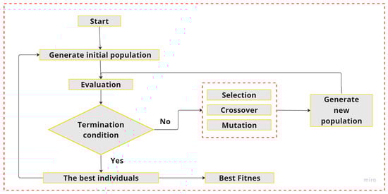
Figure 1.
General flowchart of genetic algorithm.
In the algorithm used in this research (all risks are not processed at the same time and this algorithm is used for each risk separately and the results are recorded in the archive), the initial population uses a randomly generated initialization strategy that is created by randomly selecting neurons for the neural network, learning rates, activation functions, and regularization techniques. It consists of N coded individuals:
In the optimization of neural networks using GA, the evaluation step consists of evaluating the fitness of each chromosome in the population. This step is very important in order to find the best solutions and guide the search for better solutions. When optimizing neural networks, the evaluation step usually involves training and testing the neural network using the chromosome-specified architecture. In the current case, the fitness of a population in Ga is based on the prediction error. The fitness value of each chromosome () can be calculated as follows:
Moreover, the selection operator () of this individual is:
where is the fitness value of the chromosome, is the number of ANN input data, is the GA population size, and is the error of the ANN input corresponding to the chromosome [54].
Crossover recombines information from the two best parent solutions into what we hope are even better offspring solutions. The problem is to design a crossover operator that combines the features of both parent individuals.
For the real-code GA, the crossover operator includes simple, arithmetic, and heuristic crossovers. In the present study, the arithmetic crossover was used. Therefore, suppose and are two parent chromosomes selected for the application of the crossover operator and two offspring, namely, and ; they are built as follows:
Here, is a random number from an interval that remains constant for uniform arithmetic crossover or varies based on the number of generations for non-uniform arithmetic crossover.
The mutation operation randomly changes the value of each chromosome element according to the mutation probability. For the real-code GA, the mutation operators include uniform, non-uniform, multi-non-uniform, boundary, etc. In the present research, the non-uniform mutation was used.
Assume as a chromosome and as a gene to be mutated. Then, the gene is as follows:
in which:
Here, and are the lower and upper bounds of each variable, respectively. and are the number of current generations and the maximum number of generations, respectively. and are two random numbers between (0 and 1). Moreover, is a user-selected parameter that determines the degree of dependency on the number of iterations [55,56,57].
3. Description of the Proposed New Model
In this article, the authors attempt to design an optimal neural network architecture that exhibits significant performance on various FMEA risk datasets. While neural networks can learn transferable features, such as changes in data distribution, specific features of the original domain, noise levels, and data size, dimensionality can impair the effectiveness of a pre-trained neural architecture [58]. However, different datasets using the same neural architecture may not always yield the desired results. In other words, it is impossible to present a unique architecture for all the risks studied in this research with the greatest accuracy. Hence, to achieve optimal performance, the customization of the neural architecture is essential [54]. To overcome this challenge, we propose the concept of dataset-specific architecture design, which includes adjusting the network’s depth, width, activation functions, and regularization techniques to match the characteristics of the dataset. Therefore, the innovation of the current research, which distinguishes it from other studies, is the design of a neural network architecture by optimizing all hyperparameters, while previous studies focused on one or two effective parameters. Designing the proposed optimal neural network architecture is very challenging because it involves choosing the appropriate hyperparameters and optimizing the model performance. The traditional customized GA design provides a systematic and automated approach for exploring the vast search space of possible network architectures and hyperparameters. Through their evolutionary nature, GAs can effectively converge to optimal solutions [59,60]. In summary, the schematic of the proposed new model is demonstrated in Figure 2.
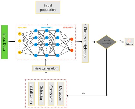
Figure 2.
Schematic of the proposed new model.
As shown in Figure 2, there are input data to the system that include various types of risk. Moreover, each risk has a subset of a number of questions. On the other hand, the number of strings of each entry is different. Therefore, this algorithm was used for each risk separately and the results are stored in the PyTorch model. It should be remembered that the PyTorch model is not suitable for running on a mobile application and it is necessary to make changes to the output, which will be discussed in detail in the next step. Moreover, details of this structure are complex, and it is not possible to see all of it in the schematic figure above, especially the gray block that acts like a black box. Therefore, more details of this proposed methodology are presented below.
GA operates by exploring and exploiting based on the encoding method, which consists of three main steps: selection, crossover, and mutation. On the other hand, the neural network contains various hyperparameters, including network topology selection, which affects the prediction accuracy. The parameters of the applied GAs are given in Table 1.

Table 1.
Genetic algorithm settings and the parameters used to evolve the best neural network architecture and their associated values.
In the last step, the GA finds the best architecture and hyperparameters for each FMEA risk separately.
4. Experimental Data and Implementation of the Proposed Algorithm
As stated before, the aim of this research is to create a new practical methodology for forecasting with a trained model using the model server method. Here, the server can be a cloud-based server, an on-premises server, or even a specialized machine designed to provide machine-learning models [61,62]. To interact with the deployed model, it is necessary to create an API that enables communication between the client of an application and the server hosting the model. Since the client’s request was to design a mobile application, using the server method had several problems. The advantages and disadvantages of using this method are summarized in Table 2.
Table 2.
Comparison of the server and the embedded method used in the present research.
Embedded models on devices offer several advantages over the server-based method [63]. By running the model locally on the device, latency is minimized and enables real-time processing for the application. When the model is on the server, the data transfer is carried out through the Internet platform and the TCP protocol, and it takes time, but, when it is carried out on the mobile phone, the models are optimized and is on the dataset; therefore, it uses the mobile processor and performs the next calculations instantly. Since sensitive information remains on the device, data privacy and security are enhanced. Offline operation becomes feasible and ensures performance in disconnected environments. Additionally, reduced server costs, lower bandwidth usage, and alignment with edge computing principles make embedded models an efficient choice, provided challenges such as limited device resources and model updates are properly addressed. The next step is to choose a platform for working with neural networks. The options are usually considered between IOS and Android operating systems. We selected the iPhone (with IOS) for several reasons, such as fewer models available on the iPhone platform. However, they are more standard and have more processing power. On the iPhone platform, there are three types of chips, including neural engine, which is especially suitable for neural network tasks [64,65]. After selecting the platform, we need to decide on a framework for implementing neural networks. To this end, we chose Core ML to work with the Neural Engine on Apple devices, as it effectively uses the computational capabilities of the Neural Engine and integrates tightly with Apple ecosystem. As a result, it facilitates the development of machine-learning applications. Core ML also supports on-device inference, which is essential for real-time applications, and provides model optimization capabilities that enable the efficient use of hardware acceleration [66]. Notably, the choice between Core ML and other technologies, such as TensorFlow Lite [67], OpenVINO [68], and Nvidia Jetson [69] depends on the application and specific task requirements. Each of these frameworks has its own features and advantages, and the best choice is determined based on the specific needs of the project. To better understand this issue, Figure 3 presents the conversion and optimization diagram of the PyTorch model to the Corel ML for the embedded device.
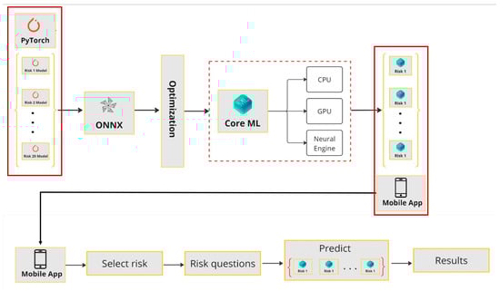
Figure 3.
Conversion and optimization diagram of the PyTorch model to the Corel ML for embedded device.
PyTorch is a versatile open-source machine-learning library developed by Facebook’s AI Research lab. Its dynamic computational graph feature allows on-the-fly graph creation during runtime, providing flexibility and ease of debugging. PyTorch provides powerful tensor operations similar to NumPy and supports automatic differentiation through its auto package, simplifying gradient computation for neural networks. It provides the building blocks of neural networks, including modules for defining layers, loss functions, and optimization algorithms. PyTorch seamlessly integrates with CUDA for GPU acceleration, enabling faster training.
The next step is to convert the model from PyTorch [70] to Core ML. Here, there are challenges because PyTorch is based on dynamic graphs, while Core ML works with static graphs (which are essential for model optimization). Therefore, we have to choose an intermediate format. As such a format, we used Open Neural Network Exchange (ONNX) [71]. Exporting from PyTorch is straightforward, as a result of the ‘torch-onnx’ module. Then, we improve the models using custom optimizations with the help of the ‘onnx-simplifier’ module. Subsequently, we integrated our trained models into Swift to develop a mobile application. As shown in the lower part of Figure 3, the user selects a risk category in the application interface and responds to the corresponding question associated with that specific risk. Afterward, the user will promptly receive the prediction result.
The project under consideration is a case study started by a well-known company in Russia (i.e., Blagoveshchensk, Amur region). This project was completed in 14 months and was one of the largest industrial structures in the world. The two building yards constitute approximately 32,000 m2 of the total construction space. Since concrete is the primary building material, each yard has three structures, each with six floors.
This team consists of 12 experts: one customer representative, one project manager, one worker officer, four occupational health and safety engineers, three quality engineers, one architect, and one design engineer. Members continuously monitor the work performed on the building site. Consequently, they may provide significant information that supports this case study. The team collaborated to collect the data needed to perform the re-reporting. We collected data for 20 FEMA risks. Moreover, we started the process by compiling a list of questions and criteria required for each risk (see Appendix A). Each question was scored in the range of 0–10. Subsequently, the experts recorded all the data over the course of a year. Afterward, we generated a dedicated neural network training dataset. In a neural network, the data are randomly divided into three categories: training data (70% of the data), testing data (20% of the data), and validation data (10% of the data). After obtaining the ANN model, its efficiency was assessed by calculating the Root Mean Square Error (RMSE) [72]:
The RMSE is a criterion used to optimize variance and assigns weight to errors with larger absolute values. This criterion is commonly used as a standard statistical metric to evaluate model performance. In addition, the RMSE is less sensitive to outliers than the Mean Square Error (MSE), as the former takes the square root of the MSE, and reduces the impact of large errors on the final metric [73]. When dealing with a large number of samples, the use of RMSE is considered more reliable for the error distribution.
5. Results
A large number of simulations were performed considering different architectures for the neural network, as well as the number of hidden layers in it. Such a comprehensive analysis was very time-consuming and computationally expensive (see Appendix B). Moreover, the specifications of the system used to run various codes are as follows:
- ✓
- Processor 12th Gen Intel(R) Core(TM) i9-12900H 2.90 GHz
- ✓
- Installed RAM 32.0 GB (31.7 GB usable)
- ✓
- System type 64-bit operating system, x64-based processor
- ✓
- GPU NVIDIA GeForce RTX 3080 Ti Laptop GPU
Table 3 presents the RMSE value for each type of risk in different neural network architectures with optimal hyperparameters.
Table 3.
The results obtained from different simulations for various risk categories.
As is clear from the results, even for the one hidden layer, it is not possible to find the optimal neural network architecture that covers all the risks. For example, if the number of hidden layers is considered to be 1 and the number of neurons is also considered to be 512, then, for different risks, the neural network architecture will be different again because the activation functions will be different. Therefore, we will realize the shining point of this research, that it is necessary to optimize all hyperparameters in a neural network architecture, including the number of hidden layers, the number of neurons in each layer, and the activation functions. Hence, finding a neural network with constant architecture for all risks is impossible. Moreover, it can be seen that the accuracy of the neural network cannot be directly attributed to each of the hyperparameters separately. For example, from Table 3, the optimum number of neutrons for one risk is 64, and, for another risk, the number of hidden layers is 3. It means that the accuracy does not always increase with the increase in the number of neurons or in the number of hidden layers. Therefore, it is emphasized that the accuracy of the new methodology presented in this article is significantly higher than other non-combined methods. To prove this statement, the first risk was analyzed according to the usual methods, and, using the comparison technique, the percentage of improvement in the prediction accuracy of the new methodology was investigated, the results of which are given in Appendix C.
Apart from the above explanations, the relationship between the iterations of the genetic algorithm and the RSME value, as well as the optimal points for each risk in different layers, is displayed in Figure 4. Next, Table 4 presents the standard deviation values of the dataset characteristics and objectives for each specific risk. This information provides insights into the variability and spread of the data points within each risk category, helping to better understand the distribution of data and potential risks associated with it.
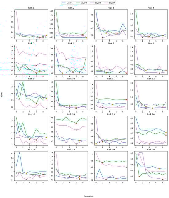
Figure 4.
The relationship between the iterations of the genetic algorithm and the RMSE value.
Table 4.
Standard deviation values for each characteristic of risks.
In Figure 4, each part contains several color charts. The legend is located at the top, which separates the number of hidden layers. For example, the blue lines represent analyses for different risks with a neural network including one hidden layer. Moreover, in each risk, various analyses were performed for four different states of hidden layers (i.e., one, two, three, and four layers), and, for every state, there is an optimal point that detects the interaction between the hyperparameters in such a way that the neural network model has the highest prediction accuracy. These points are also shown in the Figure 4. As is clear from this figure, it confirms the previous statement (in relation to Table 3) because the co-ordinates of the optimal points are not the same in all parts and diagrams.
From Table 4, the value of the standard deviation is high for the architecture with different hidden layers. It should be noted that, if a unique architecture was used for all risks, then this value would be too small for one risk and too high for another risk. Therefore, these values are obtained based on the presented methodology. Another reason for this is the nature of the risks, which are different from each other, and, since this research was based on industrial data, it was not possible to use better data and the fact was reported. Another reason is the scattering of data in each of the evaluation questions in a risk. This issue can be seen in different industries. For example, in the issue of the fatigue phenomenon in engineering, according to the ISO-1143 standard, the acceptable amount of scattering is reported to be 50%. Now, in this research, we delved into the amount of evaluation for a question: one expert can give a full score of one and another expert can give a score of zero, which creates exactly the same conditions as mentioned.
Finally, Figure 5 illustrates the Kernel Density Estimation (KDE) [74] of the features of the dataset for each specific risk, highlighting the distribution and density of the data points. In fact, it represents the relationship between the KDE graphs and the hidden layers of the neural network and explains how data features correspond to the intermediate processing layers of the network.
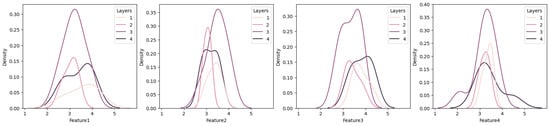
Figure 5.
KDE graphs for each risk across neural network layers.
6. Discussion
This paper develops an optimal neural network architecture for FMEA data analysis to predict risks in diverse datasets. In the proposed method, since the training data show changes in data distribution, noise levels, and scatter, among other factors, using the same neural network architecture often reduces its effectiveness and performance and leads to unsatisfactory results. This problem is solved by using an accurate selection of the hyperparameter for the neural network. Typically, this is carried out by experts in the field of neural networks who rely on their extensive personal experience. The proposed method uses GA to find the optimal architecture separately for each data type by determining the relevant hyperparameters. As shown in Table 3, this approach yielded the best and most optimal architecture for each individual FMEA risk. In addition, the running time of the code as well as the comparison of the accuracy of the proposed model with the conventional unique model are presented in Appendix B and Appendix C, respectively.
The relationship between the standard deviation of features and neural network architecture can affect the training and performance of a neural network. If the standard deviation of the input data is too high, it may be necessary to use a deeper or wider network to capture the complexity of the data. The standard deviation is often used as a measure of the spread or variability of data. Choosing the architecture (width and depth) of the neural network depends on the characteristics of the input data, such as the standard deviation. Data characteristics also affect the gradient descent method during neural network training, particularly how quickly and stably the neural network converges to the optimal weights. When the standard deviation is large, the gradients can become larger and lead to rapid weight updates. In such cases, selecting an excessively large learning rate can result in divergence. High or low values of the feature can lead to vanishing or exploding gradients, creating challenges during training. Therefore, choosing appropriate weight initialization methods, data normalization techniques, and optimization methods is very important to successfully train a network.
Next, we employed a method that enabled data processing in embedded devices. This choice was motivated by the need to prioritize data privacy, especially since FMEA information typically contains sensitive company data. Users are generally opposed to transmitting their confidential information to external servers. We converted the trained neural network model from PyTorch to Core ML and improved the models through custom optimizations using the ‘onnx-simplifier’ module. As a result, this model gained the ability to predict data on embedded devices in real time and significantly improved the speed and accuracy.
7. Conclusions
In this article, the use of artificial intelligence algorithms for risk assessment was comprehensively studied. Traditionally, risk calculation often relies on the expertise of specialists. However, this approach is costly and time-consuming. Moreover, since it often includes subjective factors such as expert opinions, experience level, and psychological pressures, it can create negative biases in risk assessment. Therefore, an artificial intelligence system based on neural networks was employed to address these challenges. One of the critical aspects of using neural networks is designing the network architecture to achieve the highest performance of the quality. For this purpose, the search for the optimal architecture and hyperparameters was automated using a GA, an evolutionary algorithm. Various experiments were conducted to evaluate this approach in 20 different types of risk. Finally, a system that enables the offline execution of the trained neural network model was used after recognizing the highly confidential nature of risk information for companies. This system processes data in embedded devices without transmitting data to external servers and ensures data privacy. Based on the analysis of risk data, significant interdependence between risks in a specific domain was identified. Using this insight, we recommend designing a neural network using a tensor that can accommodate multimodal capabilities. By simultaneously exploiting the full potential of all available symmetry information, a holistic core can be created that integrates the most influential aspects of different risks for superior results. As a result, the proposed neural network architecture promises to improve risk assessment processes and achieve more accurate predictions by using combined knowledge from diverse risk domains.
Author Contributions
Conceptualization, N.R. and K.R.K.; methodology, N.R.; software, N.R.; validation, O.A.S.; formal analysis, N.R.; investigation, N.R., L.H., M.N. and K.R.K.; resources, R.G.; data curation, O.A.S. and L.H.; writing—original draft preparation, N.R.; writing—review and editing, K.R.K.; visualization, N.R. and K.R.K.; supervision, N.R.; project administration, R.G.; funding acquisition, R.G. All authors have read and agreed to the published version of the manuscript.
Funding
This publication has been supported by the RUDN University Scientific Projects Grant System, project N° “202192-2-000”.
Data Availability Statement
The datasets can be made available upon request from the first author.
Conflicts of Interest
The authors declare no conflicts of interest.
Abbreviations
| FMEA | Failure Mode and Effect Analysis |
| GA | Genetic Algorithm |
| HACCP | Hazard Analysis and Critical Control Points |
| AI | Artificial Intelligence |
| DNN | Deep Neural Network |
| FIS | Fuzzy Inference System |
| SVM | Support Vector Machine |
| ReLU | Rectified Linear Unit |
| ELU | Exponential Linear Unit |
| SELU | Scaled Exponential Linear Unit |
| SGD | Stochastic Gradient Descent |
| Adam | Adaptive Moment Estimation |
| RMSprop | Root Mean Square Propagation |
| ONNX | Open Neural Network Exchange |
| RMSE | Root Mean Square Error |
| MSE | Mean Square Error |
| KDE | Kernel Density Estimation |
Appendix A
The list of questions and criteria considered to evaluate each risk (collected data for use in the neural network as input parameters) is as follows (Table A1):
Table A1.
List of different risks along with questions.
Table A1.
List of different risks along with questions.
| No. | Risk | Question |
|---|---|---|
| 1 | Latency and real-time processing |
|
| 2 | Compressed gas explosion |
|
| 3 | Compressor accidents |
|
| 4 | Construction project delivery failed on time |
|
| 5 | Crane accidents |
|
| 6 | Crane falls on construction site |
|
| 7 | Cutting and nail-gun accidents |
|
| 8 | Dust, noise, and vibration |
|
| 9 | Electric shock |
|
| 10 | Electrocutions |
|
| 11 | Hit by falling objects |
|
| 12 | Holes in flooring of the construction site |
|
| 13 | Run over by operating equipment |
|
| 14 | Scaffolding accidents |
|
| 15 | Scaffolding falls |
|
| 16 | Solid waste and water waste |
|
| 17 | Structure failure |
|
| 18 | Toxic and suffocation |
|
| 19 | Welding accidents |
|
| 20 | Falling of the workers from high floors |
|
Appendix B
The runtime (seconds) for the codes written in order to obtain the most optimal neural network architecture considering different numbers of hidden layers is as follows (Table A2):
Table A2.
Runtime of different algorithms according to the risk (unit is in seconds).
Table A2.
Runtime of different algorithms according to the risk (unit is in seconds).
| No. | Risk | Number of Hidden Layers | |||
|---|---|---|---|---|---|
| 1 | 2 | 3 | 4 | ||
| 1 | Latency and real-time processing | 6517 | 8774 | 11781 | 15420 |
| 2 | Compressed gas explosion | 6536 | 8616 | 11848 | 14941 |
| 3 | Compressor accidents | 6542 | 8568 | 12038 | 15029 |
| 4 | Construction project delivery failed on time | 6534 | 8675 | 12188 | 14971 |
| 5 | Crane accidents | 6519 | 8676 | 12058 | 15079 |
| 6 | Crane falls on construction site | 6568 | 8566 | 11997 | 14869 |
| 7 | Cutting and nail-gun accidents | 6529 | 8604 | 12211 | 15084 |
| 8 | Dust, noise, and vibration | 6534 | 8682 | 12203 | 14900 |
| 9 | Electric shock | 6569 | 8848 | 12158 | 14830 |
| 10 | Electrocutions | 6575 | 8895 | 11925 | 14955 |
| 11 | Hit by falling objects | 6543 | 8612 | 12220 | 15037 |
| 12 | Holes in flooring of the construction site | 6569 | 8630 | 12171 | 15138 |
| 13 | Run over by operating equipment | 6542 | 8656 | 12164 | 15046 |
| 14 | Scaffolding accidents | 6571 | 8705 | 12296 | 14985 |
| 15 | Scaffolding falls | 6541 | 8586 | 12120 | 15029 |
| 16 | Solid waste and water waste | 6532 | 8918 | 12206 | 14821 |
| 17 | Structure failure | 6535 | 8605 | 11859 | 14937 |
| 18 | Toxic and suffocation | 6537 | 8587 | 12153 | 15147 |
| 19 | Welding accidents | 6604 | 9027 | 12893 | 14192 |
| 20 | Falling of the workers from high floors | 6555 | 8875 | 12328 | 14749 |
As is clear from the results, with the increase in the number of hidden layers, the solution time increases, and the computational costs also increase.
Appendix C
To compare the accuracy improvement of the proposed method, i.e., the optimized neural network architecture by considering all hyperparameters with the conventional neural network architecture (the activation function of ReLU), the analysis for the first risk of the data collected in this research was carried out. The following figure shows the schematic of the mental idea for the proposed neural network architecture (a), the conventional neural network architecture considering a specific activation function (b), and, finally, the optimal neural network architecture obtained in this research (c).
| (a) | 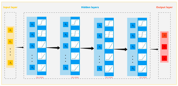 |
| (b) | 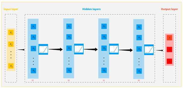 |
| (c) | 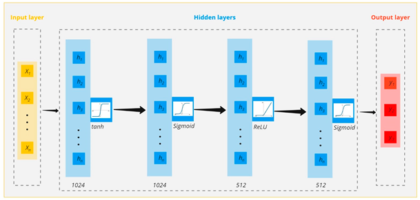 |
The result of this comparison is as follows:
| Risk No. | Number of Hidden Layers | Initialization Architecture | RMSE | Best Architecture | RMSE | Improvement (%) |
| 1 | 1 | [32, ReLU] | 0.8619 | [512, Sigmoid] | 0.2451 | 71.52 |
| 2 | [32, ReLU, 32, ReLU] | 0.7366 | [32, ‘ReLU’, 64, ‘Sigmoid’] | 0.3335 | 54.72 | |
| 3 | [32, ReLU, 32, ReLU, 32, ReLU] | 0.8011 | [1024, ‘Sigmoid’, 32, ‘Tanh’, 128, ‘ReLU’] | 0.2205 | 72.47 | |
| 4 | [32, ReLU, 32, ReLU, 32, ReLU, 32, ReLU] | 0.7489 | 1024, ‘Tanh’, 1024, ‘Sigmoid’, 512, ‘ReLU’, 512, ‘Sigmoid’] | 0.1817 | 75.73 |
References
- Maleki, E.; Unal, O.; Seyedi Sahebari, S.M.; Reza Kashyzadeh, K.; Danilov, I. Application of deep neural network to predict the high-cycle fatigue life of AISI 1045 steel coated by industrial coatings. J. Mar. Sci. Eng. 2022, 10, 128. [Google Scholar] [CrossRef]
- Amiri, N.; Farrahi, G.H.; Kashyzadeh, K.R.; Chizari, M. Applications of ultrasonic testing and machine learning methods to predict the static & fatigue behavior of spot-welded joints. J. Manuf. Process. 2020, 52, 26–34. [Google Scholar] [CrossRef]
- Kashyzadeh, K.R.; Ghorbani, S. New neural network-based algorithm for predicting fatigue life of aluminum alloys in terms of machining parameters. Eng. Fail. Anal. 2023, 146, 107128. [Google Scholar] [CrossRef]
- Fahmi, A.T.W.K.; Reza Kashyzadeh, K.; Ghorbani, S. Fault Detection in the Gas Turbine of the Kirkuk Power Plant: An Anomaly Detection Approach Using DLSTM Autoencoder. Eng. Fail. Anal. 2024, 160, 108213. [Google Scholar] [CrossRef]
- Fahmi, A.T.W.K.; Reza Kashyzadeh, K.; Ghorbani, S. Enhanced-ARIMA Model for Anomaly Detection in Power Plant Operations. Int. J. Eng. 2024; in press. [Google Scholar]
- Mikulak, R.J.; McDermott, R.; Beauregard, M. The Basics of FMEA, 2nd ed.; Taylor & Francis Group: Abingdon, UK, 2017. [Google Scholar] [CrossRef]
- Mohammadfam, I.; Gholamizadeh, K. Assessment of Security Risks by FEMA and Fuzzy FEMA Methods, A Case Study: Combined Cycle Power Plant. J. Occup. Hyg. Eng. 2021, 8, 16–23. [Google Scholar] [CrossRef]
- Xu, Z.; Dang, Y.; Munro, P.; Wang, Y. A Data-Driven Approach for Constructing the Component-Failure Mode Matrix for FMEA. J. Intell. Manuf. 2020, 31, 249–265. [Google Scholar] [CrossRef]
- Wessiani, N.A.; Yoshio, F. Failure Mode Effect Analysis and Fault Tree Analysis as a Combined Methodology in Risk Management. IOP Conf. Ser. Mater. Sci. Eng. 2018, 337, 012033. [Google Scholar] [CrossRef]
- Arvanitoyannis, I.S.; Varzakas, T.H. Application of ISO 22000 and Failure Mode and Effect Analysis (FMEA) for Industrial Processing of Salmon: A Case Study. Crit. Rev. Food Sci. Nutr. 2008, 48, 411–429. [Google Scholar] [CrossRef] [PubMed]
- Baybutt, P. Calibration of Risk Matrices for Process Safety. J. Loss Prev. Process Ind. 2015, 38, 163–168. [Google Scholar] [CrossRef]
- Maleki, E.; Unal, O.; Seyedi Sahebari, S.M.; Reza Kashyzadeh, K. A novel approach for analyzing the effects of almen intensity on the residual stress and hardness of shot-peened (TiB + TiC)/Ti–6Al–4V composite: Deep learning. Materials 2023, 16, 4693. [Google Scholar] [CrossRef] [PubMed]
- Maleki, E.; Unal, O.; Sahebari, S.M.S.; Kashyzadeh, K.R.; Amiri, N. Enhancing Friction Stir Welding in Fishing Boat Construction through Deep Learning-Based Optimization. Sustain. Mar. Struct. 2023, 5, 1–14. [Google Scholar] [CrossRef]
- Li, M.; Andersen, D.G.; Smola, A.J.; Yu, K. Communication Efficient Distributed Machine Learning with the Parameter Server. In Proceedings of the Advances in Neural Information Processing Systems 27: Annual Conference on Neural Information Processing Systems 2014, Montreal, QC, Canada, 8–13 December 2014; Volume 27. [Google Scholar]
- Wu, X.; Wu, J. The Risk Priority Number Evaluation of FMEA Analysis Based on Random Uncertainty and Fuzzy Uncertainty. Complexity 2021, 2021, 8817667. [Google Scholar] [CrossRef]
- Rafie, M.; Samimi Namin, F. Prediction of Subsidence Risk by FMEA Using Artificial Neural Network and Fuzzy Inference System. Int. J. Min. Sci. Technol. 2015, 25, 655–663. [Google Scholar] [CrossRef]
- Ku, C.; Chen, Y.S.; Chung, Y.K. An Intelligent FMEA System Implemented with a Hierarchy of Back-Propagation Neural Networks. In Proceedings of the 2008 IEEE Conference on Cybernetics and Intelligent Systems, Chengdu, China, 21–24 September 2008; pp. 203–208. [Google Scholar] [CrossRef]
- Okabe, T.; Otsuka, Y. Proposal of a Validation Method of Failure Mode Analyses Based on the Stress-Strength Model with a Support Vector Machine. Reliab. Eng. Syst. Saf. 2021, 205, 107247. [Google Scholar] [CrossRef]
- Maleki, E.; Kashyzadeh, K.R. Effects of the hardened nickel coating on the fatigue behavior of CK45 steel: Experimental, finite element method, and artificial neural network modeling. Iran. J. Mater. Sci. Eng. 2017, 14, 81–99. [Google Scholar] [CrossRef]
- Ke, J.; Liu, X. Empirical Analysis of Optimal Hidden Neurons in Neural Network Modeling for Stock Prediction. In Proceedings of the 2008 IEEE Pacific-Asia Workshop on Computational Intelligence and Industrial Application, Wuhan, China, 19–20 December 2008; pp. 828–832. [Google Scholar] [CrossRef]
- Balaprakash, P.; Salim, M.; Uram, T.D.; Vishwanath, V.; Wild, S.M. DeepHyper: Asynchronous Hyperparameter Search for Deep Neural Networks. In Proceedings of the 2018 IEEE 25th International Conference on High Performance Computing (HiPC), Bengaluru, India, 17–20 December 2018; pp. 42–51. [Google Scholar] [CrossRef]
- Susmi, S.J. Hybrid Dimension Reduction Techniques with Genetic Algorithm and Neural Network for Classifying Leukemia Gene Expression Data. Indian J. Sci. Technol. 2016, 9, 1–8. [Google Scholar] [CrossRef]
- Sharma, K.D.; Srivastava, S. Failure Mode and Effect Analysis (FMEA) Implementation: A Literature Review. J. Adv. Res. Aeronaut. Space Sci. 2018, 5, 1–17. [Google Scholar]
- Sankar, N.R.; Prabhu, B.S. Modified Approach for Prioritization of Failures in a System Failure Mode and Effects Analysis. Int. J. Qual. Reliab. Manag. 2001, 18, 324–336. [Google Scholar] [CrossRef]
- Moreira, A.C.; Ferreira, L.M.D.F.; Silva, P. A Case Study on FMEA-Based Improvement for Managing New Product Development Risk. Int. J. Qual. Reliab. Manag. 2021, 38, 1130–1148. [Google Scholar] [CrossRef]
- Dubey, S.R.; Chakraborty, S.; Roy, S.K.; Mukherjee, S.; Singh, S.K.; Chaudhuri, B.B. DiffGrad: An Optimization Method for Convolutional Neural Networks. IEEE Trans. Neural Netw. Learn. Syst. 2020, 31, 4500–4511. [Google Scholar] [CrossRef]
- Zhang, Z. Improved Adam Optimizer for Deep Neural Networks. In Proceedings of the 2018 IEEE/ACM 26th International Symposium on Quality of Service (IWQoS), Banff, AB, Canada, 4–6 June 2018; pp. 1–2. [Google Scholar] [CrossRef]
- Ida, Y.; Fujiwara, Y.; Iwamura, S. Adaptive Learning Rate via Covariance Matrix Based Preconditioning for Deep Neural Networks. In Proceedings of the Twenty-Sixth International Joint Conferences on Artificial Intelligence Organization, Melbourne, Australia, 19–25 August 2017; pp. 1923–1929. [Google Scholar] [CrossRef]
- Yang, J.; Bagavathiannan, M.; Wang, Y.; Chen, Y.; Yu, J. A Comparative Evaluation of Convolutional Neural Networks, Training Image Sizes, and Deep Learning Optimizers for Weed Detection in Alfalfa. Weed Technol. 2022, 36, 512–522. [Google Scholar] [CrossRef]
- Vieira, S.; Lopez Pinaya, W.H.; Garcia-Dias, R.; Mechelli, A. Deep Neural Networks. Mach. Learn. Methods Appl. Brain Disord. 2020, 157–172. [Google Scholar] [CrossRef]
- Montesinos López, O.A.; Montesinos López, A.; Crossa, J. Fundamentals of Artificial Neural Networks and Deep Learning. In Multivariate Statistical Machine Learning Methods for Genomic Prediction; Springer: Cham, Switzerland, 2022; pp. 379–425. Available online: https://link.springer.com/chapter/10.1007/978-3-030-89010-0_10 (accessed on 28 August 2023).
- Janocha, K.; Czarnecki, W.M. On Loss Functions for Deep Neural Networks in Classification. arXiv 2017, arXiv:1702.05659. [Google Scholar] [CrossRef]
- Koutsoukas, A.; Monaghan, K.J.; Li, X.; Huan, J. Deep-Learning: Investigating Deep Neural Networks Hyper-Parameters and Comparison of Performance to Shallow Methods for Modeling Bioactivity Data. J. Chemin. 2017, 9, 42. [Google Scholar] [CrossRef] [PubMed]
- Huuskonen, J.; Salo, M.; Taskinen, J. Aqueous Solubility Prediction of Drugs Based on Molecular Topology and Neural Network Modeling. J. Chem. Inf. Comput. Sci. 1998, 38, 450–456. [Google Scholar] [CrossRef] [PubMed]
- Basheer, I.A.; Hajmeer, M. Artificial Neural Networks: Fundamentals, Computing, Design, and Application. J. Microbiol. Methods 2000, 43, 3–31. [Google Scholar] [CrossRef]
- LeCun, Y.; Bengio, Y.; Hinton, G. Deep Learning. Nature 2015, 521, 436–444. [Google Scholar] [CrossRef] [PubMed]
- Yu, X.; Hu, X.; Liu, Z.; Wang, C.; Wang, W.; Ghannouchi, F.M. A Method to Select Optimal Deep Neural Network Model for Power Amplifiers. IEEE Microw. Wirel. Compon. Lett. 2021, 31, 145–148. [Google Scholar] [CrossRef]
- Alvarez, J.M.; Salzmann, M. Learning the Number of Neurons in Deep Networks. Learning the number of neurons in deep networks. Adv. Neural Inf. Process. Syst. 2016, 29, 1–9. [Google Scholar]
- Sheela, K.G.; Deepa, S.N. Review on Methods to Fix Number of Hidden Neurons in Neural Networks. Math. Probl. Eng. 2013, 2013, 425740. [Google Scholar] [CrossRef]
- Shen, Z. Deep Network Approximation Characterized by Number of Neurons. Commun. Comput. Phys. 2020, 28, 1768–1811. [Google Scholar] [CrossRef]
- Zeiler, M.D.; Ranzato, M.; Monga, R.; Mao, M.; Yang, K.; Le, Q.V.; Nguyen, P.; Senior, A.; Vanhoucke, V.; Dean, J.; et al. On Rectified Linear Units for Speech Processing. In Proceedings of the 2013 IEEE International Conference on Acoustics, Speech and Signal Processing, Vancouver, BC, Canada, 26–31 May 2013; pp. 3517–3521. [Google Scholar] [CrossRef]
- Xu, J.; Li, Z.; Du, B.; Zhang, M.; Liu, J. Reluplex Made More Practical: Leaky ReLU. In Proceedings of the 2020 IEEE Symposium on Computers and Communications (ISCC), Rennes, France, 7–10 July 2020; pp. 1–7. [Google Scholar] [CrossRef]
- Ding, B.; Qian, H.; Zhou, J. Activation Functions and Their Characteristics in Deep Neural Networks. In Proceedings of the 2018 Chinese Control and Decision Conference (CCDC), Shenyang, China, 9–11 June 2018; pp. 1836–1841. [Google Scholar] [CrossRef]
- Kiliçarslan, S.; Celik, M. RSigELU: A Nonlinear Activation Function for Deep Neural Networks. Expert. Syst. Appl. 2021, 174, 114805. [Google Scholar] [CrossRef]
- Khan, S.H.; Hayat, M.; Porikli, F. Regularization of Deep Neural Networks with Spectral Dropout. Neural Netw. 2019, 110, 82–90. [Google Scholar] [CrossRef] [PubMed]
- Yang, T.; Zhu, S.; Chen, C. Gradaug: A New Regularization Method for Deep Neural Networks. Adv. Neural Inf. Process. Syst. 2020, 33, 14207–14218. [Google Scholar]
- Nusrat, I.; Jang, S.-B. A Comparison of Regularization Techniques in Deep Neural Networks. Symmetry 2018, 10, 648. [Google Scholar] [CrossRef]
- Yazan, E.; Talu, M.F. Comparison of the stochastic gradient descent based optimization techniques. In Proceedings of the 2017 International Artificial Intelligence and Data Processing Symposium (IDAP), Malatya, Turkey, 16–17 September 2017; pp. 1–5. [Google Scholar] [CrossRef]
- Qian, N. On the Momentum Term in Gradient Descent Learning Algorithms. Neural Netw. 1999, 12, 145–151. [Google Scholar] [CrossRef]
- Dogo, E.M.; Afolabi, O.J.; Nwulu, N.I.; Twala, B.; Aigbavboa, C.O. A Comparative Analysis of Gradient Descent-Based Optimization Algorithms on Convolutional Neural Networks. In Proceedings of the 2018 International Conference on Computational Techniques, Electronics and Mechanical Systems (CTEMS), Belgaum, India, 21–22 December 2018; pp. 92–99. [Google Scholar] [CrossRef]
- Kurbiel, T.; Khaleghian, S. Training of Deep Neural Networks Based on Distance Measures Using RMSProp. arXiv 2017, arXiv:1708.01911. [Google Scholar] [CrossRef]
- Lambora, A.; Gupta, K.; Chopra, K. Genetic Algorithm- A Literature Review. In Proceedings of the 2019 International Conference on Machine Learning, Big Data, Cloud and Parallel Computing (COMITCon), Faridabad, India, 14–16 February 2019; pp. 380–384. [Google Scholar] [CrossRef]
- Katoch, S.; Chauhan, S.S.; Kumar, V. A Review on Genetic Algorithm: Past, Present, and Future. Multimed. Tools Appl. 2021, 80, 8091–8126. [Google Scholar] [CrossRef]
- Reza Kashyzadeh, K.; Amiri, N.; Ghorbani, S.; Souri, K. Prediction of Concrete Compressive Strength Using a Back-Propagation Neural Network Optimized by a Genetic Algorithm and Response Surface Analysis Considering the Appearance of Aggregates and Curing Conditions. Buildings 2022, 12, 438. [Google Scholar] [CrossRef]
- Whitley, D.; Sutton, A.M. Genetic Algorithms—A Survey of Models and Methods. In Handbook of Natural Computing; Springer: Berlin/Heidelberg, Germany, 2012; pp. 637–671. [Google Scholar]
- Kim, Y.K.; Song, W.S.; Kim, J.H. A Mathematical Model and a Genetic Algorithm for Two-Sided Assembly Line Balancing. Comput. Oper. Res. 2009, 36, 853–865. [Google Scholar] [CrossRef]
- Stepanov, L.V.; Koltsov, A.S.; Parinov, A.V.; Dubrovin, A.S. Mathematical Modeling Method Based on Genetic Algorithm and Its Applications. J. Phys. Conf. Ser. 2019, 1203, 012082. [Google Scholar] [CrossRef]
- Chen, G.; Fu, K.; Liang, Z.; Sema, T.; Li, C.; Tontiwachwuthikul, P.; Idem, R. The Genetic Algorithm Based Back Propagation Neural Network for MMP Prediction in CO2-EOR Process. Fuel 2014, 126, 202–212. [Google Scholar] [CrossRef]
- David, O.E.; Greental, I. Genetic Algorithms for Evolving Deep Neural Networks. In Proceedings of the Companion Publication of the 2014 Annual Conference on Genetic and Evolutionary Computation, Vancouver, BC, Canada, 12–16 July 2014; pp. 1451–1452. [Google Scholar] [CrossRef]
- Pham, T.A.; Tran, V.Q.; Vu, H.-L.T.; Ly, H.-B. Design Deep Neural Network Architecture Using a Genetic Algorithm for Estimation of Pile Bearing Capacity. PLoS ONE 2020, 15, e0243030. [Google Scholar] [CrossRef] [PubMed]
- Verhelst, M.; Moons, B. Embedded Deep Neural Network Processing: Algorithmic and Processor Techniques Bring Deep Learning to IoT and Edge Devices. IEEE Solid-State Circuits Mag. 2017, 9, 55–65. [Google Scholar] [CrossRef]
- Loni, M.; Sinaei, S.; Zoljodi, A.; Daneshtalab, M.; Sjödin, M. DeepMaker: A Multi-Objective Optimization Framework for Deep Neural Networks in Embedded Systems. Microprocess. Microsyst. 2020, 73, 102989. [Google Scholar] [CrossRef]
- Hou, X.; Breier, J.; Jap, D.; Ma, L.; Bhasin, S.; Liu, Y. Security Evaluation of Deep Neural Network Resistance Against Laser Fault Injection. In Proceedings of the 2020 IEEE International Symposium on the Physical and Failure Analysis of Integrated Circuits (IPFA), Singapore, 20–23 July 2020; pp. 1–6. [Google Scholar] [CrossRef]
- Izbassarova, A.; Duisembay, A.; James, A.P. Speech Recognition Application Using Deep Learning Neural Network. In Deep Learning Classifiers with Memristive Networks; Springer: Cham, Switzerland, 2020; pp. 69–79. [Google Scholar]
- Dlužnevskij, D.; Stefanovič, P.; Ramanauskaité, S. Investigation of YOLOv5 Efficiency in IPhone Supported Systems. Balt. J. Mod. Comput. 2021, 9, 333–344. [Google Scholar] [CrossRef]
- Sujaini, H.; Ramadhan, E.Y.; Novriando, H. Comparing the Performance of Linear Regression versus Deep Learning on Detecting Melanoma Skin Cancer Using Apple Core ML. Bull. Electr. Eng. Inform. 2021, 10, 3110–3120. [Google Scholar] [CrossRef]
- David, R.; Duke, J.; Jain, A.; Reddi, V.J.; Jeffries, N.; Li, J.; Kreeger, N.; Nappier, I.; Natraj, M.; Regev, S.; et al. TensorFlow Lite Micro: Embedded Machine Learning on TinyML Systems. Proc. Mach. Learn. Syst. 2021, 3, 800–811. [Google Scholar]
- Demidovskij, A.; Gorbachev, Y.; Fedorov, M.; Slavutin, I.; Tugarev, A.; Fatekhov, M.; Tarkan, Y. OpenVINO Deep Learning Workbench: Comprehensive Analysis and Tuning of Neural Networks Inference. In Proceedings of the 2019 IEEE/CVF International Conference on Computer Vision Workshop (ICCVW), Seoul, Republic of Korea, 27–28 October 2019; pp. 783–787. [Google Scholar]
- Mittal, S. A Survey on Optimized Implementation of Deep Learning Models on the NVIDIA Jetson Platform. J. Syst. Archit. 2019, 97, 428–442. [Google Scholar] [CrossRef]
- Imambi, S.; Prakash, K.B.; Kanagachidambaresan, G.R. PyTorch. In Programming with TensorFlow: Solution for Edge Computing Applications; Springer: Cham, Switzerland, 2021; pp. 87–104. [Google Scholar] [CrossRef]
- Jin, T.; Bercea, G.-T.; Le, T.D.; Chen, T.; Su, G.; Imai, H.; Negishi, Y.; Leu, A.; O’Brien, K.; Kawachiya, K.; et al. Compiling ONNX Neural Network Models Using MLIR. arXiv 2020, arXiv:2008.08272. [Google Scholar] [CrossRef]
- Chai, T.; Draxler, R.R. Root Mean Square Error (RMSE) or Mean Absolute Error (MAE)?—Arguments against Avoiding RMSE in the Literature. Geosci. Model. Dev. 2014, 7, 1247–1250. [Google Scholar] [CrossRef]
- Wang, W.; Lu, Y. Analysis of the Mean Absolute Error (MAE) and the Root Mean Square Error (RMSE) in Assessing Rounding Model. IOP Conf. Ser. Mater. Sci. Eng. 2018, 324, 012049. [Google Scholar] [CrossRef]
- Chen, Y.-C. A Tutorial on Kernel Density Estimation and Recent Advances. Biostat. Epidemiol. 2017, 1, 161–187. [Google Scholar] [CrossRef]


Disclaimer/Publisher’s Note: The statements, opinions and data contained in all publications are solely those of the individual author(s) and contributor(s) and not of MDPI and/or the editor(s). MDPI and/or the editor(s) disclaim responsibility for any injury to people or property resulting from any ideas, methods, instructions or products referred to in the content. |
© 2024 by the authors. Licensee MDPI, Basel, Switzerland. This article is an open access article distributed under the terms and conditions of the Creative Commons Attribution (CC BY) license (https://creativecommons.org/licenses/by/4.0/).