Abstract
Economic and policy factors are driving the continuous increase in the adoption and usage of electrical vehicles (EVs). However, despite being a cleaner alternative to combustion engine vehicles, EVs have negative impacts on the lifespan of microgrid equipment and energy balance due to increased power demands and the timing of their usage. In our view, grid management should leverage on EV scheduling flexibility to support local network balancing through active participation in demand response programs. In this paper, we propose a model-free solution, leveraging deep Q-learning to schedule the charging and discharging activities of EVs within a microgrid to align with a target energy profile provided by the distribution system operator. We adapted the Bellman equation to assess the value of a state based on specific rewards for EV scheduling actions and used a neural network to estimate Q-values for available actions and the epsilon-greedy algorithm to balance exploitation and exploration to meet the target energy profile. The results are promising, showing the effectiveness of the proposed solution in scheduling the charging and discharging actions for a fleet of 30 EVs to align with the target energy profile in demand response programs, achieving a Pearson coefficient of 0.99. This solution also demonstrates a high degree of adaptability in effectively managing scheduling situations for EVs that involve dynamicity, influenced by various state-of-charge distributions and e-mobility features. Adaptability is achieved solely through learning from data without requiring prior knowledge, configurations, or fine-tuning.
1. Introduction
The ongoing transition towards various economic sectors’ decarbonization enables fossil energy-supply substitution with renewable energy. However, the rapid adoption of small-scale renewables at the edge of the grid makes the smart grid management process more complex and exposed to uncertainties related to renewable production [1,2]. Digitization and decentralization principles bring, to the forefront, energy demand flexibility as a key support to accommodate high shares of variable renewable energy [3,4]. Leveraging local flexibility is possible to maintain a balance between supply and demand at lower costs using the energy assets of citizens rather than the ones owned by grid operators, which are more expensive to operate [5,6,7]. In this context, demand response programs have been defined by grid operators for adjusting the consumer’s electricity patterns in response to the fluctuations in renewable energy production. Consumers are requested to shift their flexible energy usage to times when renewable energy is produced in excess or reduce consumption during peak demand.
The challenges are even more evident and difficult to tackle in the context of the increased adoption of electrical vehicles (EVs) [8]. Usually, electric vehicles need to be charged daily. They have a substantial amount of flexibility to be used in demand response programs if their charging and discharging are smartly planned.
In this respect, grid management should closely cooperate and interact within a low latency context with EV coordination and aggregation services to procure their energy scheduling flexibility to support local network balancing or to achieve self-sufficiency [9,10]. However, EV usage has several shortcomings such as a limited battery range, a relatively short battery lifespan, averaging 10–20 years or up to 150,000 miles, and a lack of existing infrastructure for charging electric vehicles. Other major issues refer to the impact of EVs on the power grid, encompassing factors such as the rise in short-circuit currents, deviations in voltage levels beyond standard limits, and the potential impact on the lifespan of equipment due to increased power demands [11]. Studies have shown that fully charging an electric vehicle uses the same energy needed to power a home during peak energy use times, and nowadays, the energy grid cannot deal with a major or sudden spike in EV usage [12]. Moreover, this is not only a problem related to the quantity of electricity consumed by EVs but also the timing of their usage [13]. If many electric vehicles were to be charged in the evening, the grid could experience significant strain, potentially leading to blackouts.
To address the challenges of EV coordination for smart grid management, demand response programs are used to convince people to change their energy behavior [14]. Dynamic traffic for electricity is well discussed in the literature as a solution to move the charging schedules of EVs to moments of the day with extra solar energy [15]. However, it still faces open challenges related to the complexity of the pricing structure that involves hourly or time-of-use rates, making EV owners reluctant to engage and requiring EV owners to adapt their behavior based on fluctuating electricity prices [16]. Other solutions are leveraging on the setup of demand response programs for EVs aiming to manage and modify their charging or discharging patterns based on grid conditions [17]. However, this presents a major challenge: the need to balance energy production and consumption in the face of intermittent and non-programmable energy sources which are strongly influenced by atmospheric conditions, making this difficult to predict [2].
In terms of algorithms for smart scheduling and the coordination of EV participation in DR programs, many existing state-of-the-art approaches consider variations of the model-based constraint-satisfaction problem [18]. They provide a structured framework for considering various constraints and optimization objectives including grid capacity, user preferences, and energy prices. They achieve good results; however, their main drawbacks are related to the model’s assumptions and structure, which need to be continuously updated to meet the actual changing conditions in grid states, charging station deployments, and EV availability [19]. Moreover, the model solving method is computationally complex, being less suitable for large-scale dynamic features involved in EV scheduling [20].
In this paper, we address the limitations by proposing a model-free solution for EV participation in DR programs, leveraging deep Q-learning. We aim to schedule the charging and discharging activities of EVs within a microgrid to align with a target energy profile provided by the grid operator for a specific interval. The deep Q-learning solution determines optimal EV scheduling actions based only on the current state, which is represented by the state of charge of EVs and the availability of charging stations in the microgrid. We adapted the Bellman equation, which plays a crucial role in assessing the value of a specific state, considering specific rewards for EV scheduling actions and Q-values to evaluate the effectiveness of each action. The methodology typically involves the estimation of Q-values for available EV scheduling actions and then the selection of the actions with the highest reward. Traditionally, the Q-function is implemented as a look-up table, updated after each transition. However, in dynamic scenarios with a multitude of complex states, rendering a table insufficient, we opt for representing the Q-function using a neural network in which the input variables signify the state, and the output provides the Q-value for every possible action. For action selection, we employed the epsilon-greedy algorithm to balance the exploitation of the current best action or explore new possibilities for EV scheduling to meet the target DR energy profile.
The main advantage of our model-free solution compared to model-based solutions is that it can learn from previous experiences, which allows it to make better decisions over time about scheduling EVs at charging stations. Also, model-free solutions can learn optimal scheduling policies that yield good results when operating in complex and uncertain environments or with frequent changes. Finally, model-free solutions do not require prior knowledge and are consequently able to dynamically adapt to different scheduling scenarios without having to have a predefined model.
The rest of this paper is structured as follows: Section 2 reviews the literature on EV scheduling and coordination solutions; Section 3 presents our deep Q-learning solution for EV participation in DR programs; Section 4 provides experimental validation, demonstrating the approach’s effectiveness in meeting target energy profiles and evaluating the quality of the learned EV scheduling solutions; and Section 5 concludes the paper and presents future work.
2. Related Work
Reinforcement learning-based approaches (RLs) for EV scheduling have been studied in the literature to optimize the charge and discharge decisions in a dynamic and uncertain environment. Wen et al. [21] schedule electric vehicles for charging and discharging using a deep Q-learning-based method that considers both the mobility of electric vehicles and the random charging behavior of users. The EV’s scheduling is made by considering a distribution model for user charging times, a model for charging demands, a dynamic model for EV state of charge, and a model for travel locations. A dynamic reward function, the electricity price, the charging and discharging cost, and the battery degradation cost are employed to optimally schedule EVs, such that the economic operating cost is reduced, and the efficiency of the charging/discharging process is improved. However, this method suffers from a drawback, namely, the dynamic reward function does not accurately reflect the benefits of charging/discharging operations when user behavior deviates from the assumptions made in the travel location model. Lee et al. [22] also propose a deep RL-based method for EV charging and discharging in real time. The aim is to minimize the EVs’ charging cost and to reduce grid loads during peak hours. To model the usage patterns of charging stations, a parametric density function estimation is used that allows the learning agents to make optimal charging and discharging decisions. The effectiveness of this approach has been demonstrated through simulations, and the results demonstrate that a significant reduction in the energy cost and the grid load is obtained. Wan et al. [23] combine a representation network with deep RL to schedule the charging and discharging of electric vehicles in a domestic setting, such that the EVs’ charging/discharging cost is minimized. The representation network (i.e., LTSM network) is used to extract features from historical electricity prices that, together with the EVs’ battery SoC and user driving patterns (i.e., the arrival and departure times), are given as inputs to the Q-learning network to estimate the optimal action-value function. Like in the previous work, the effectiveness of this approach has also been demonstrated through simulation. In their work, Viziteu et al. [24] use deep Q-learning to schedule EVs for charging by considering the battery SoC, the battery capacity, the longest trip distance, the distance between the EVs’ current location and the charging station, the waiting time until the next charging slot is available, and the charging station power. The aim is to manage electric vehicle congestion by scheduling them in advance at charging stations and optimizing drivers’ journeys. Like in the case of previous approaches, this approach’s effectiveness has been demonstrated through simulations. Cao et al. [25] address the problem of scheduling electrical vehicles for charging, aiming to reduce carbon emission costs and peak loads in a community. The proposed approach integrates three algorithms: an offline scheduling algorithm that considers EV profiles, the EVs’ random arrivals, and power constraints to minimize the carbon emission cost; an online heuristic rolling-based scheduling algorithm that considers the EVs’ arrival times and SoC to make carbon emission decisions; and an actor–critic RL scheduling algorithm that updates the EV carbon emission actions. This approach has been tested through simulations. Liu et al. [26] schedule EVs for charging to minimize the cost of charging EVs and stabilizing the voltage of the distribution network. The scheduling and voltage-control problems are modeled as a Markov decision process that considers the uncertainty introduced by the charging behavior of electric vehicle drivers and an uncontrolled load, as well as fluctuations in energy prices and renewable energy production. The deep deterministic policy gradient algorithm is used to return discrete and continuous control actions. The reward function is defined to ensure a balance between EV charging and voltage stability. Paraskevas et al. [27] introduce a win–win strategy based on deep Q-learning (DLR), aiming to maximize both the charging station’s profits and drivers’ charging demands. The DRL agent’s decisions are taken in real-time by considering the uncertainties due to future EV-arrival distribution and electricity prices. Wang et al. [28] propose an improved rainbow-based deep RL strategy for the optimal scheduling of charging stations. The charging process, involving the matching between EV-charging demands and CS equipment resources, is modeled as a finite Markov decision process. To schedule EVs at charging stations under uncertain conditions due to EV arrival and departure times, a DQN-based rainbow algorithm is used. Li et al. [29] propose an approach for the optimal scheduling of electric vehicles for charging/discharging to minimize charging costs and to ensure the full charging of electric vehicles. The EV charging/discharging scheduling problem is defined as a constrained Markov decision process, where the constraints are the full charging of EVs and the minimization of charging costs and is solved using a secure deep RL strategy. An electric vehicle aggregator (EVA) is proposed in [30] as the decision-making authority for scheduling electric vehicles for charging. Scheduling is performed considering uncertainties related to renewable energy generation and user demands and has, as its main objectives, a minimization of the cost of EVA and fluctuations in the power exchange of the microgrid. The EV charge-scheduling problem is modeled as a Markov decision-making process based on deep RL and is solved using a twin delayed deep deterministic policy gradient algorithm. Heendeniya et al. [31] introduce a DRL technique based on the actor–critic architecture for the optimal charging of electric vehicles. The aim is to minimize both the charging time and expected voltage violations. The proposed technique can learn an optimal policy by considering the voltage magnitude measurements and improve the scalability by imposing partial observability. Shi et al. [32] propose an RL-based approach for managing a community’s electric vehicle fleet that offers ride-hailing services to residents. The aim is to minimize the clients’ waiting time, the electricity cost, and vehicles’ operational costs. To solve the problem of dispatching the electric vehicle fleet, decentralized learning is combined with centralized decision making. Decentralized learning allows EVs to share their knowledge and learned models to estimate the state-value function, while centralized decision making assures EV coordination to avoid scheduling conflicts. Li et al. [33] propose a strategy for charging EVs, aiming at achieving the main goal of EV-charging-cost minimization. This strategy uses JANET to extract regular variability in energy prices and deep RL to adjust the charging strategy of EVs based on variability in energy prices. Ding et al. [34] also propose a strategy for charging electric vehicles to increase the profit of distribution system operators while ensuring the correct use of distribution networks to avoid potential voltage problems. A model based on Markov decision making is defined to describe the uncertainty of EV-user behavior, and a learning algorithm based on deterministic political gradients is used to solve the model. Park et al. [35] solve the problem of scheduling EVs for charging through a deep learning-based method of multi-agent reinforcement, in which the training stage is centralized, and the execution stage is decentralized. The aim is to minimize the operating costs of charging stations and to ensure the amount of energy specified for charging EVs.
However, even though model-free reinforcement learning solutions are promising for EV scheduling and smart grid management due to their ability to adapt to variable conditions and uncertainties in renewable generation, they also feature challenges that are partially addressed in this paper. Reinforcement learning algorithms require many samples, episodes, and action simulations to learn the optimal EV scheduling policies. The convergence of rewards and losses to desirable values, even in our solution, was a process that took a considerable number of learning episodes. Moreover, in most cases, achieving a good balance between exploration (i.e., trying new EV scheduling actions) and exploitation (i.e., leveraging on known actions) is rather challenging. We addressed this by employing an epsilon-greedy strategy and fine-tuning the delicate balance between the exploitation and exploration of the EV scheduling search space. Another challenge in the studied literature is the reward function design for the objectives of EV scheduling. We addressed this by adapting the Bellman equation to evaluate the EV scheduling state from an energy perspective and defined a Q-function to determine the EV scheduling effectiveness for the DR program. Finally, the state and action spaces in EV scheduling can be high dimensional and complex, making it challenging for the Q-learning network to efficiently learn the optimal policy for DR, thus requiring the fine-tuning of the learning and network architecture parameters.
3. Deep Q-Learning for EV Energy Scheduling
The objective of EV scheduling is to be able to participate collectively in demand response programs (DRs) used to balance the supply and demand of electricity in the smart grid [36]. We considered V2G-enabled EVs (Vehicle to Grid) [37] that can respond to grid operator signals by modifying their energy consumption or generation patterns. We formalize a DR program as follows:
where is a goal energy curve provided to the participant EVs. A Q-learning algorithm determines the collective response of EVs.
In Q-learning, one popular assumption is that the environment in which the agent learns is described as a Markov decision process. We will use this simplifying assumption, which means that the future state of the environment depends only on the previous states and actions of the agent. We formally define the environment in which the agent acts as follows:
where is the state space, representing the set of possible states that the agent might be in; is the action space, representing the set of all possible actions that the agent can take when it is in each state; is the policy that the agent learns; and r is the rewards given to the agents as results of his actions.
The state space represents all possible mappings of EVs on charging stations over the demand response program interval . We model it as a matrix with the dimensions :
where is the number of available charging stations, and is the number of timeslots for DR. An element of the matrix stores the identity of the EV, which is assigned to a charging station at specific timeslots or otherwise zero:
For each environment state, the equivalent energy state is determined and stored in a HashMap , in which the set of keys are the individual timeslots in the DR program interval , and the list of values represent the energy charged or discharged at each charging point:
The amount of energy charged or discharged in total by all charging stations in the microgrid per a time slot is determined as follows:
The initial state of the agent exploration process is represented by a matrix with zero values, indicating that no EVs are assigned to any charging station within the interval . The agent will explore and learn by performing actions, receiving rewards based on these actions and updating the Q-values. An action corresponds to assigning an electric vehicle to a charging station in a certain timeslot :
When the agent performs an action, it results in a new state, which is represented as a new matrix containing the new configuration of electric vehicles assigned to charging stations. This iterative process allows the agent to learn the optimal policy for assigning electric vehicles to charging stations while considering the specific constraints and the objective defined for our problem.
In the defined environment, we considered several constraints on the set of actions the agent may consider to be driven by the physical limitations of the energy infrastructure. The type of action for an EV at a charging station at a time slot can be either a charge or a discharge:
An EV will be considered for scheduling only if its current state of charge falls within a predefined range based on its capacity, and this is correlated with the types of associated actions:
The electric vehicle will only be eligible for charging if its is significantly less than the maximum capacity and for discharging if the is significantly higher than the minimum capacity.
Two different EVs, and , cannot be scheduled at the at the same charging station in the same time slot :
Finally, the amount of energy charged or discharged by EVs at a timeslot must not exceed the target energy provided by the grid operator in the DR program:
The goal of the agent is to find new environmental states by successively simulating the execution of actions, such that the distance between the target energy curve and the amount of energy charged and discharged by EVs is minimized over the DR program interval :
Moreover, the agent goal is to learn an optimal policy, , that maximizes the cumulative reward obtained by executing a sequence of actions in the defined environment. To find the optimal policy, the agent explores the environment, observes the rewards obtained when taking specific actions in each state, and uses this experience to update his knowledge of the best actions taken in different states. The optimal policy has associated an optimal that represents the maximum return that can be obtained from a state , taking an action and subsequently following the optimal policy:
The optimal action-value function is described by the Bellman equation, which establishes a link between the optimal action value of one state–action pair and the optimal action value of the next state–action pair.
where is the new Q-value calculated for the action ; is the learning rate; is the immediate reward; is the discount rate; and is the maximum Q-value selected from all Q -values obtained by executing all possible actions in the next state . In our model, we set the initial Q-value of a pair as usually initialized with an arbitrary fixed value before learning begins.
The immediate rewards assigned to a state–action pair are as follows:
Figure 1 shows an overview of the Q-Learning model defined for EV coordination for DR participation.
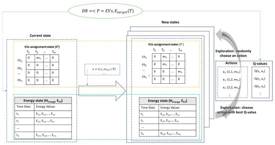
Figure 1.
The Q-Learning model.
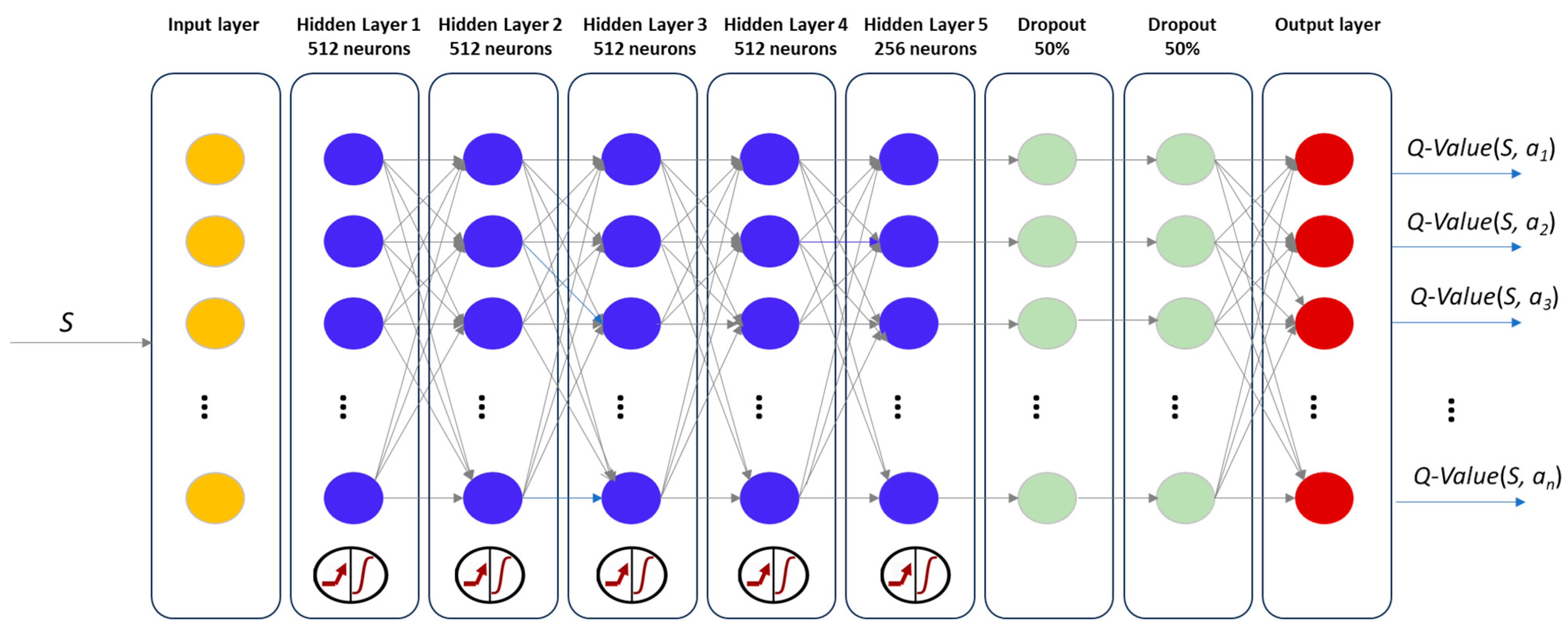
The Q-function is modeled using a deep neural network (Q-network), having, as input, the states (i.e., EV mapping to charging stations and time slot states) and outputs the associated Q-value. To train the neural network, we use the -greedy algorithm [38] to ensure that the exploration–exploitation strategies are balanced. It helps to balance the trade-off between exploring unknown actions and exploiting the ones with the best Q-values. Figure 2 shows the structure of the Q-network used.
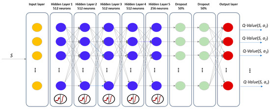
Figure 2.
Q-network used for Q-function approximation.
The deep Q network architecture was developed through experimentation, learning from previous trials, and adapting to the specific requirements of EV charging and discharging scheduling for demand response. This architecture consists of five dense hidden layers with ReLU activation: four layers with 512 neurons and one with 256 neurons. We chose this architecture to strike a balance between expressiveness and computational efficiency, considering that too few neurons can lead to underfitting, while too many can lead to overfitting or an increased computational cost. It also includes two dropout layers, each with a dropout rate of 0.5 to prevent overfitting. There is an input layer matching the size of the state space and an output layer matching the size of the action space, representing the Q-value for each possible action in the environment.
In the learning process, we also used a target Q-network (TQ-network) with the same architecture as the Q-network. Its weights are updated more slowly and periodically with the weights from the Q-network. The TQ-network is used for stabilizing the learning process and improving the algorithm’s efficiency by updating the network after a certain number of iterations instead of after every episode. Both the Q-network architecture and the target Q-network will be initialized with the same randomly generated weights.
The deep Q-learning model for EV scheduling in demand response is presented in Algorithm 1. The Q-network architecture and the TQ-network are initialized, and the network weights are randomly generated (lines 1–5).
| Algorithm 1 Deep Q-Learning for EV Scheduling |
| Inputs: S—state space, A—action space, CS—the set of charging stations, EV—the set of electrical vehicles, T—the time slots, N—the number of epochs for model training, —DR program target curve Outputs: —the weights of the TQ-network Q-network parameters: the weights of the network, epsilon parameter, D—replay memory, m—target network update frequency, —learning rate, discount factor Begin |
The replay memory is initialized and updated in the learning process with the tuples containing the transitions from one state to another, as well as the rewards given to these transitions. A Boolean variable is defined for situations in which the training episode is over: either when all electric vehicles have been assigned to a charging station in a specific time slot or when two electric vehicles have been assigned to the same charging station at the same time slot. The batch size variable is used to determine how many entries from the replay memory are randomly selected to be used for training the model.
After completing the initialization, the model training process starts, and the agent interacts with the defined scheduling environment. Initially, it reads the initial state of the environment before the scheduling (lines 3–4), which includes the scheduling matrix of electric vehicles at the charging stations, together with the DR program’s target energy profile. An action is selected based on the ϵ-greedy method to ensure the balance between exploration and exploitation for model training (lines 7–11). A random number between 0 and 1 is generated and then compared to the value of the hyperparameter , which is originally initialized with 1. In case the random value is smaller than , the action is chosen randomly, without considering the reward obtained. If the value is greater than , the action with the biggest Q-value for the current state is selected. The action selected by the agent is executed by updating the scheduling matrix. The reward is calculated, and the next state is updated with the current EV planning matrix (line 12), and the information is stored in the replay memory. Since the size of the resume memory is fixed, when the number of transitions in the memory exceeds its size, the oldest value is removed.
Then, for the training process, we randomly extract a mini-batch sample of transitions from the replay memory D of the size of the batch (lines 16–24). This step is only performed once there are enough transitions in the memory to cover the batch size. The Q-values from the TQ-network are determined from stored transitions from the previous step, and the Q-values from the Q-network are determined based on the original network (18–19). Afterward, we determine the loss by using the mean squared difference between the TQ-values and Q-values and calculate the loss gradients relative to the Q-network weights (lines 20–21). The new weights of the model are determined considering η: a hyperparameter representing the learning rate of the network in which the weights are updated. The weights of the Q-network are updated based on the calculated gradients, and after each m episode, the weights of the current Q-network are copied to the target Q-network to improve the accuracy of the target network for future training (lines 22–23). Finally, the value of the ϵ parameter is updated via a constant decay rate, and the TQ-network parameters are returned.
4. Evaluation Results
In this section we evaluate and test the effectiveness and efficiency of our EV scheduling method described in Section 3 for implementing demand response programs. We have used a data set of EVs, and for each EV, the following information is available: vehicle ID; model; battery power, expressed in kW; the battery capacity, expressed in kWh; the connector type; and the state of charge of the battery, expressed in percentages. The following types of EVs are considered: (a) Renault ZOE, with a battery capacity of 22 kWh and a maximum charge power of 22 kW; (b) Renault ZOE, with a battery capacity of 41 kWh and a maximum charge power of 22 kW; and (c) Nissan LEAF, with a battery capacity of 24 kWh and a maximum charge power of 7 kW.
We started the evaluation process by first setting up the configuration environment (see Table 1). The state-of-charge (SoC) values of electric vehicles (EVs) in this environment configuration follows a random distribution.

Table 1.
Environment configuration, actions, and DR program.
In our study, we explored two demand response-inspired scenarios, with the aim of balancing the electricity supply and demand in a microgrid and reducing the likelihood of failures. In the first scenario, electric vehicles are charged during periods of excess renewable energy in the microgrid, thereby adjusting the total energy demand. This aligns the energy consumption of electric vehicles with the peak of renewable energy supply. In the second scenario, energy stored in electric vehicles is discharged to address grid congestion during periods when the peak energy demand exceeds actual production.
We then generated the curves for energy demand and for renewable energy production that need to be balanced through electric vehicle (EV) scheduling. The two curves were generated by simulation.
Next, we moved on to Deep Q-Network (DQN) training. In the training process we considered the following input features for model learning: the number of available charging stations; the number of EVs waiting for charging/discharging; the time slots for scheduling; the state of charge (SoC) of each EV; the capacity of each EV; and the energy available in each time slot, representing the energy available for scheduling during that specific hour. This energy value dynamically updates every hour by (i) subtracting the energy needed to charge electric vehicles allocated to charging stations at that hour from the initial target energy value provided by the network operator in the case of charging operations or (ii) adding the energy discharged from electric vehicles allocated to charging stations at that hour to the initial target energy value provided by the network operator in the case of discharging operations. In the training process, the DQN relies on the replay memory, which stores the agent’s past experiences. After completing each episode, the agent selects a batch of experiences from this memory and uses it to train the network. The training process of the Deep Q-Network (DQN) involves adjusting several hyperparameters in the learning process, namely, the memory size, learning rate, epsilon decay, and batch size. To identify the optimal values of these hyperparameters, we used a trial-and-error approach that involves testing different values for these parameters, observing their impact on model performance, and selecting the values that produced the best results. Table 2 shows the configurations tested and the results obtained in terms of minimum loss and maximum reward for 160,000 episodes for each considered configuration.
Table 2.
Configuration of network hyperparameters and obtained results.
In the case of memory size, we started with a small memory size, which we gradually increased, and looked at how it influenced the agent’s learning capacity. In the case of a small size, the number of experiences the agent can store is limited, and as a result, due to insufficient space exploration, the policy learned is suboptimal. In the case of a large memory size, the agent accumulates a wide range of experiences, which leads to an improvement in exploration and a reduction in the occurrence of the phenomenon of overfitting. However, too large values lead to increased computational costs. Based on these findings and considering the dimension of the environment in which the agent learns, we settled on the value of 700,000 for memory size.
The epsilon decay value was chosen as 0.99996 to promote exploration at the beginning of training and progressively reduce random decisions as the model learns. Using this value, the agent does more exploration in the initial episodes, thus gathering a wide range of transition experiences. As more episodes pass, epsilon decay gradually decreases, meaning that, over time, the agent takes fewer random actions and begins to make decisions based on information learned from the neural network. The learning rate (η) value of 0.001 was chosen, because smaller updates to model weights lead to more stable learning in complex environments, even though more training episodes are required to converge to the optimal policy.
A batch size value equal to 50,000 was chosen, as this gives the best results for loss and reward metrics. A higher value implies a learning process that converges more slowly (i.e., longer training time) and also does not effectively improve the accuracy of the results, while a smaller value would imply a learning process that converges faster but gives results less accurately.
After establishing the optimal configuration for network hyperparameters, we proceeded to evaluate the quality of the training model and of the learned policy. Table 3 presents the metrics used in the evaluation process of the trained model and learned policy.
Table 3.
Metrics used to evaluate the quality of the trained model and of the learned policy.
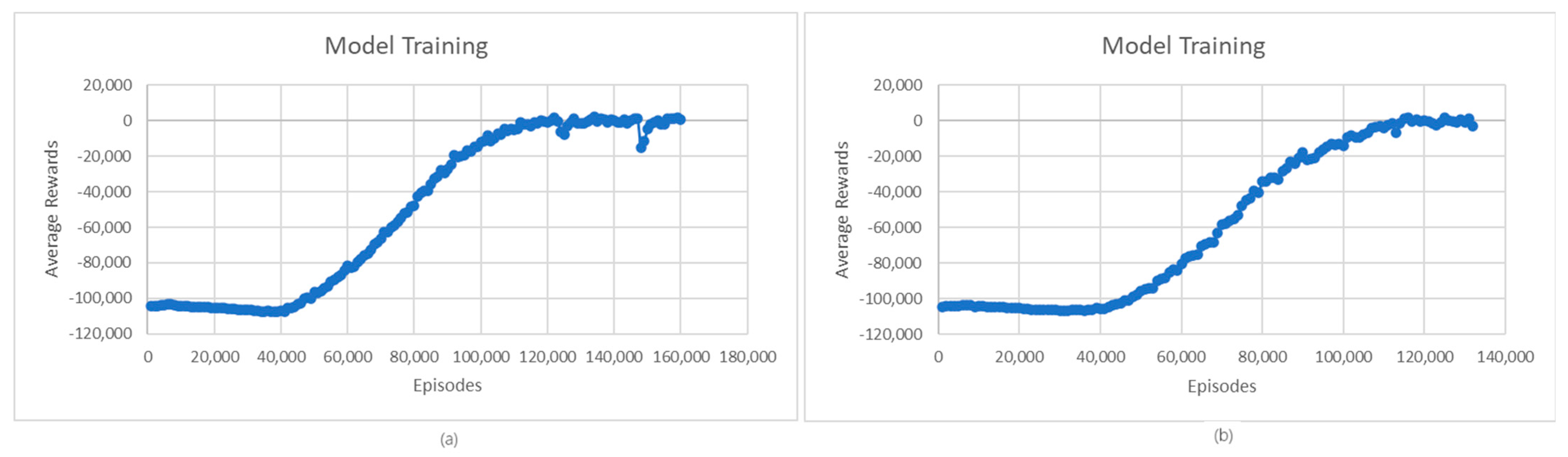
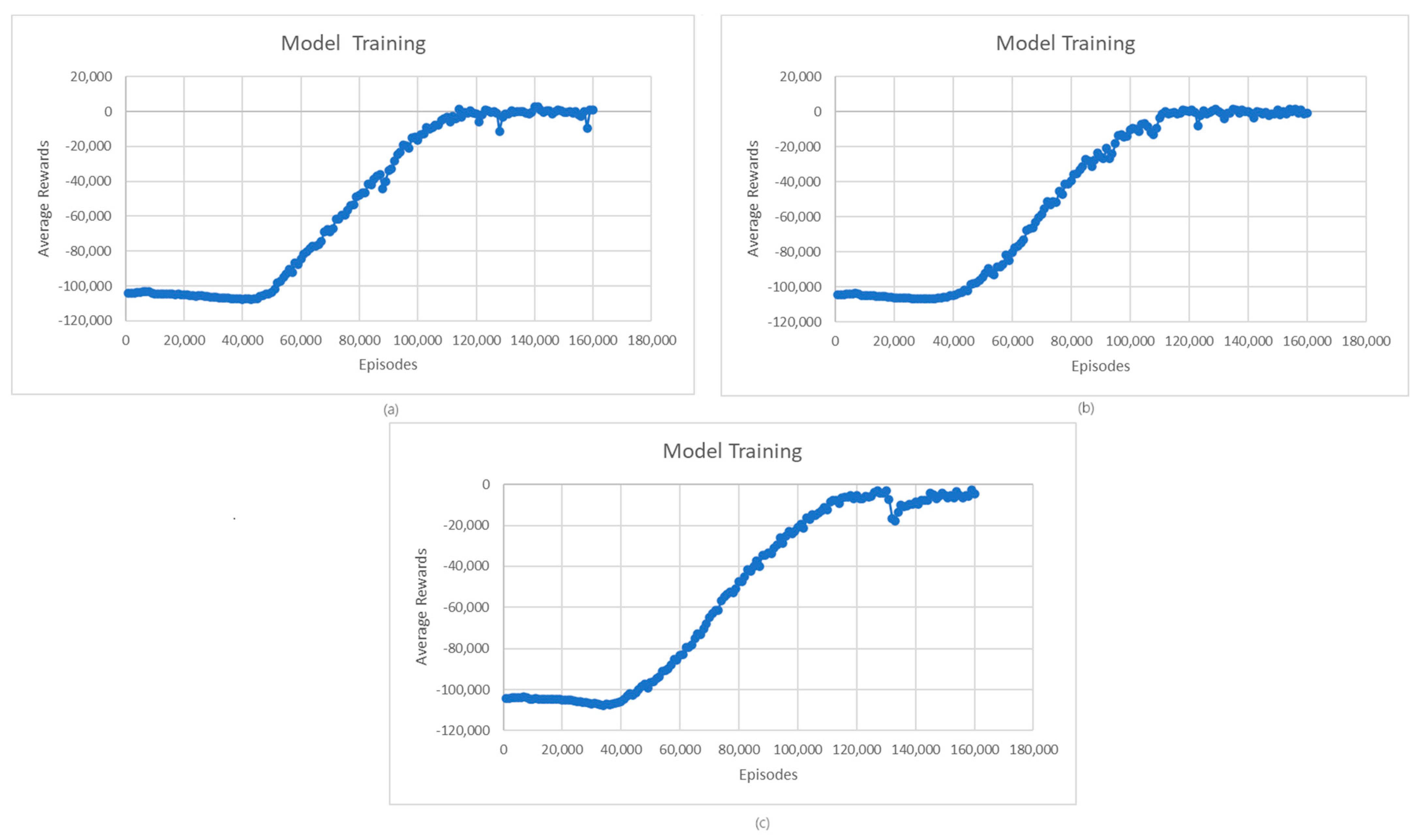
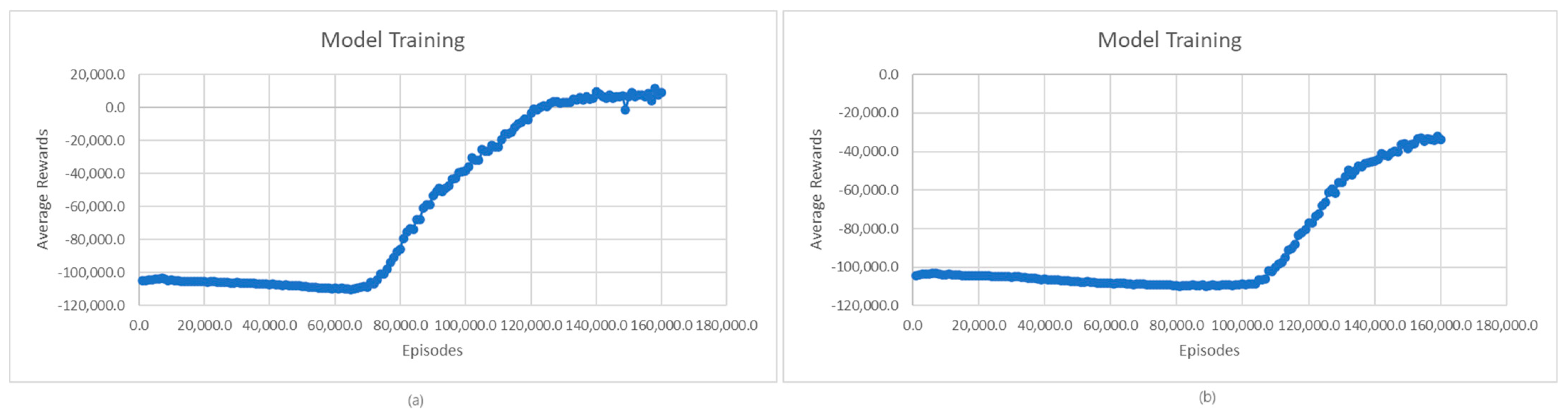
The first step in the evaluation process is the evaluation of the quality of the learned model. Figure 3 shows the evolution of average rewards during L1- and L2-model training for charging and discharging operations. In the case of the L1 model for charging, we can see that the average rewards of the learning model stabilize around 140,000 episodes; then, at 150,000, there is a temporary worsening of the received rewards, followed by a return and stabilization of the rewards starting from 16,000 episodes. This situation may be due to the complex environment in which the agent operates, which may face situations in which its performance temporarily degrades until it adapts to the new conditions. In the case of the L2 model, a significant increase in rewards is observed between 40,000 and 100,000 episodes, followed by a smaller increase between 100,000 and 120,000 episodes. Starting from episode 120,000, the reward stabilizes, registering only a few small fluctuations. Like the L1 model, these small fluctuations are due to the complexity of the environment in which the agent operates and the exploration vs. exploitation trade-off.
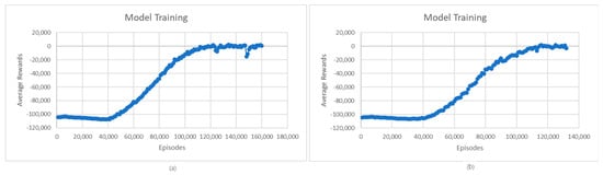
Figure 3.
(a) Average rewards for L1-model training; (b) Average rewards for L2-model training.
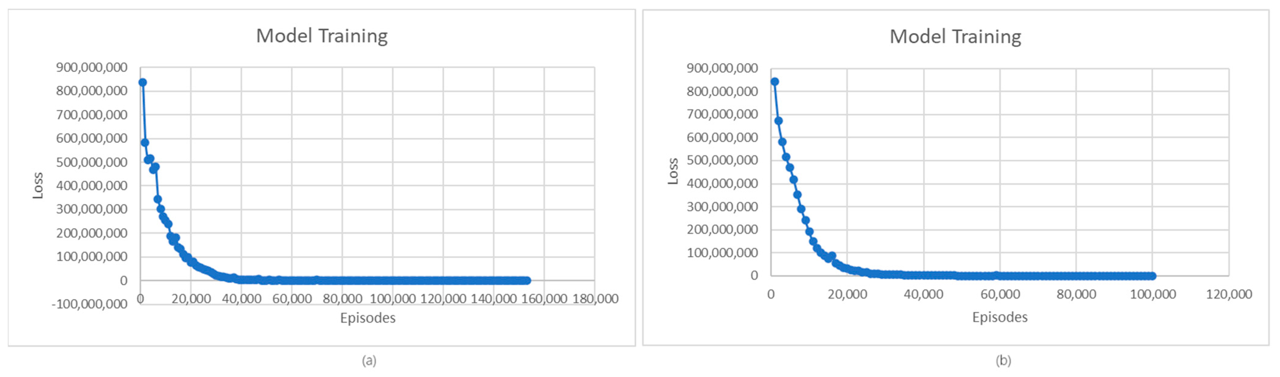
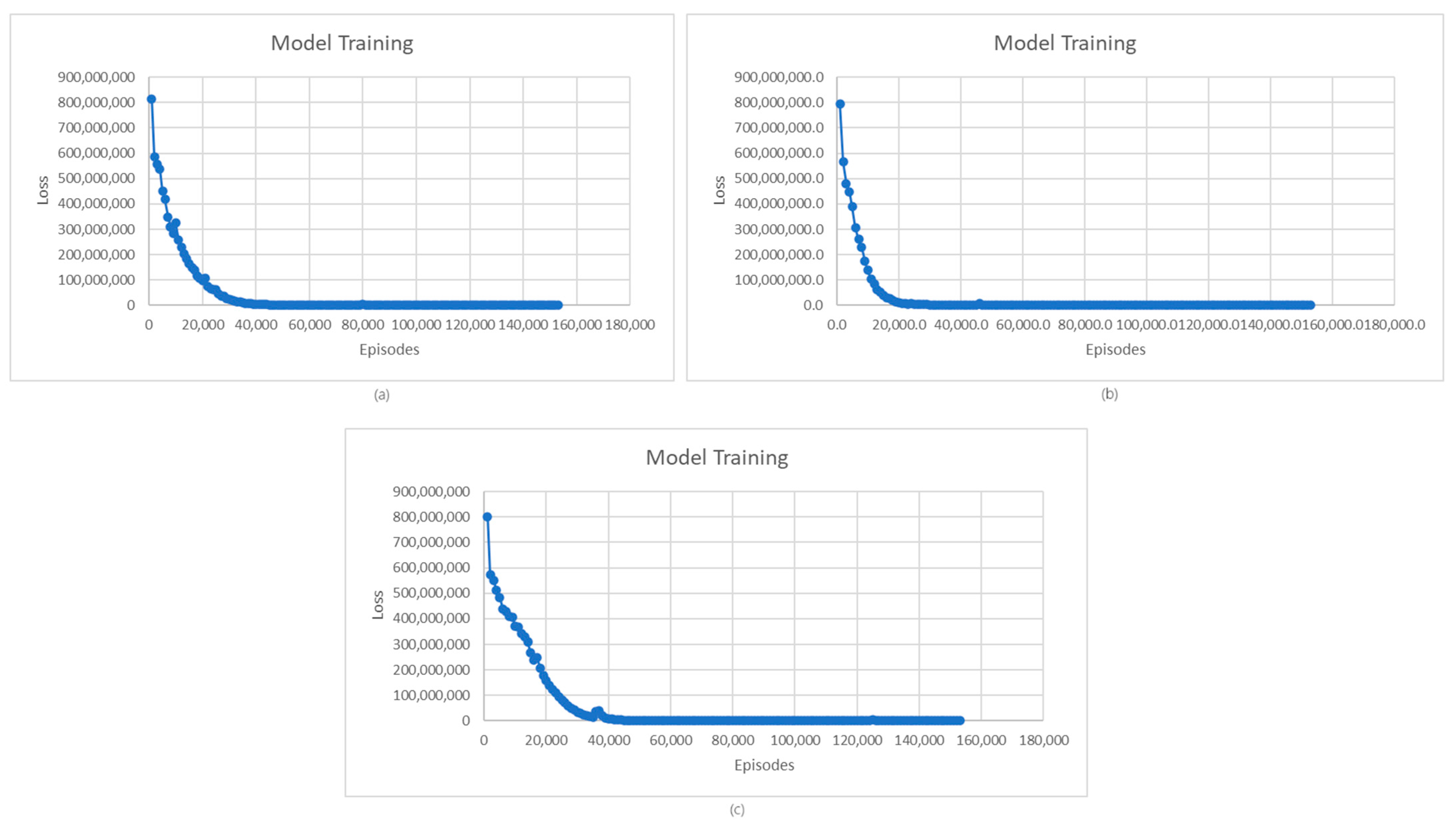
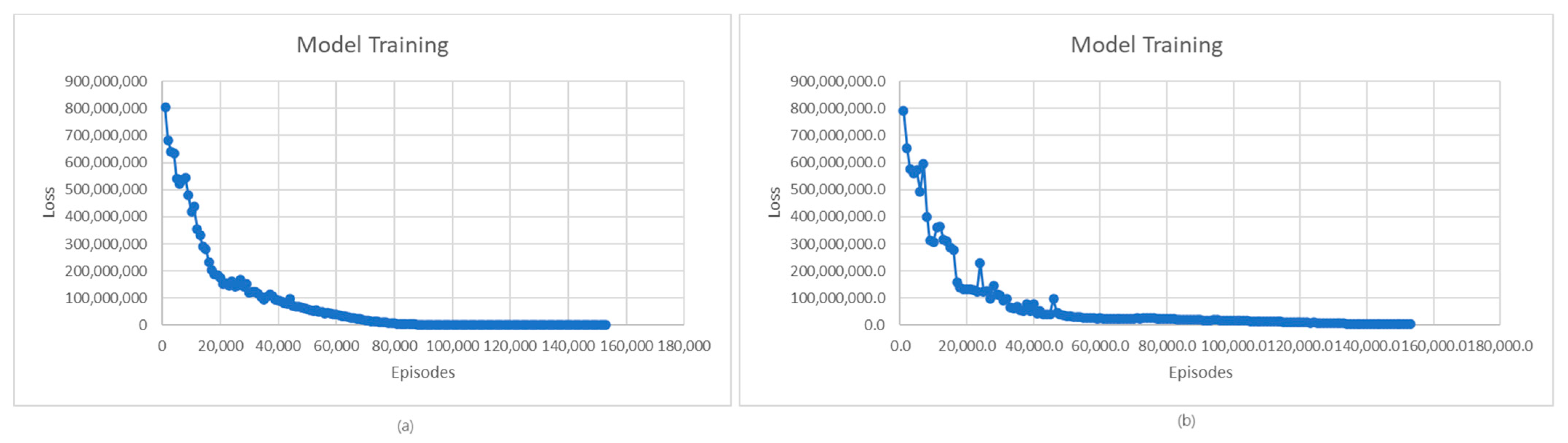
Looking at the loss evolution presented in Figure 4, we observe a common trend followed by both the L1 and L2 models. At first, the loss decreases as the models learn, and then, after many episodes, it starts to stabilize. More precisely, in the case of the L1 model, the loss starts to stabilize around 57,000 episodes and, in the case of the L2 model, around 37,000 episodes. The need for many episodes to stabilize loss derives both from the complexity of the environment in which the agent operates and from the trade-off of exploration versus exploitation. The agent needs more episodes to accumulate learning experiences and to strike the right balance between exploration and exploitation.
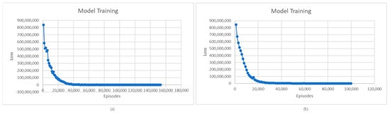
Figure 4.
(a) Average loss for L1 model; (b) Average loss for L2 model.
After evaluating the quality of the learned model, the next step is to evaluate the quality of the policy learned. For this, we examined the percentage of allocations of electric vehicles at charging stations with a maximum value of the reward, in relation to the total number of EV allocations per time interval and epoch variations. We also examined the similarity between the curve derived from the scheduling of electric vehicles at charging stations and the target energy curve provided by the grid operator using the Pearson correlation coefficient:
In Formula (17), n is the number of energy values corresponding to the time interval during which the EVs’ scheduling is performed; and are the energy data points in the goal energy curve and the curve resulted by scheduling EVs at charging stations; and and are energy sample means, computed as follows:
Figure 5 presents the percentage of optimal allocations of EVs versus suboptimal ones for the two learned policies corresponding to the charging and discharging scenarios. In the case of the charging scenario, we observe that in 70.8% of the cases, all vehicles are optimally allocated (that is, the trained model optimally manages EVs); in 17.5% of the cases, one EV is a suboptimal allocation; and in 5.6% of the cases, two EVs are suboptimal allocations. Only a small percentage of cases feature more EV suboptimal allocations (i.e., 6.1%). This means that the learned model makes good decisions, since it can optimally allocate EVs in most cases. Even when suboptimal allocations occur, their frequency is relatively low, indicating that the model has learned a policy that works well for this scenario. In the case of the L2 model, in 82.9% of the cases, EVs are optimally allocated to charging stations; in 14.4% of the cases, there is only one suboptimal allocation; and in the case of 2.5%, there are two suboptimal allocations. As in the case of the L1 scenario, the policy learned in the case of the L2 scenario can make optimal decisions in most cases, regarding the allocation of electric vehicles to the charging stations.
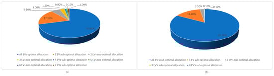
Figure 5.
(a) The percentage of optimal/suboptimal allocations of EVs for the policy learned in the case of the charging scenario; (b) The percentage of optimal/suboptimal allocations of EVs for the policy learned in the case of the discharging scenario.
The tracking of the evolution of the percentage of optimal allocations of electric vehicles over episodes is shown in Figure 6.
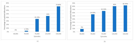
Figure 6.
(a) The evolution of the percentage of optimal allocations of electric vehicles over episodes for the L1 model; (b) The evolution of the percentage of optimal allocations of electric vehicles over episodes for the L2 model.
Examining the results obtained in the case of the L1 model, we notice that after 9500 episodes, the algorithm can optimally allocate EVs in 35.7% of the cases, reaching an optimal allocation of 70.8% after 160,000 episodes. Similarly, for the L2 model, an optimal EV allocation of 82.9% begins after 160,000 episodes. Consequently, in both models, the percentage of optimal allocations for EVs increases with each passing episode throughout the learning process, which demonstrates the effectiveness of the learned policies.
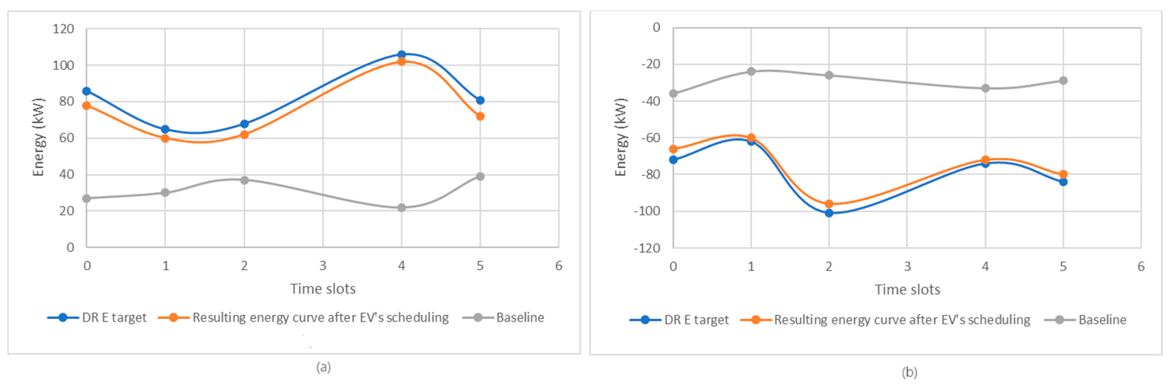
The final step of the learned-policy evaluation involves assessing the effectiveness of EV allocations at charging stations in each time slot throughout the scheduling period. Figure 7 presents the curve resulted by scheduling EVs at charging stations, together with the target energy curve provided by the grid operator, as well as the baseline curve in the case of charge and discharge scenarios. Analyzing these graphs, we notice that for both learned models (i.e., L1 and L2), the curve obtained from scheduling EVs closely follows the target energy curve provided by the grid operator. Also, when we schedule the charging/discharging of electric vehicles with our method, the resulting energy curve is much closer to the target energy curve. EV scheduling for charging/discharging significantly improves the charging/discharging capacity compared to the baseline scenario, where EV charging/discharging is conducted without any prior appointment.
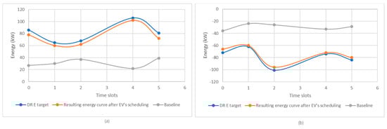
Figure 7.
(a) Comparison between the microgrid energy curve and the resulting curve after scheduling EVs in the case of the L1 model; (b) Comparison between the microgrid energy curve and the resulting curve after scheduling EVs in the case of the L2 model.
In the charging scenario, the variation between the energy required to charge electric vehicles and the energy supplied by the network operator in each time slot does not exceed a maximum deviation of 6 kW, indicating an optimal allocation of electric vehicles at charging stations. This high level of alignment between the two curves is reflected by the value of the Pearson correlation coefficient of 0.9926, which indicates a strong similarity between the energy curves. In the discharge scenario, the situation is similar. In this case, the Pearson correlation coefficient shall be 0.9937, and the variation between the energy discharged by electric vehicles and the network operator’s energy requirements during each time slot does not exceed a maximum deviation of 4 kW.
5. Discussion
Most of existing studies in EV coordination for demand response consider only charging scenarios for renewable energy integration. Moreover, they consider only a limited number of EVs and rather rigid models of the constraints and EV state-of-charge distributions, lacking adaptation features. Our approach introduces significant innovations by employing model-free reinforcement learning for the scheduling and coordination of a fleet of EVs under a V2G operation involving a bidirectional energy flow between the electric grid and EVs. Unlike model-based methods, this approach learns from past experiences in scheduling EV charging and discharging actions based on grid conditions and requirements defined in DR programs. By integrating user preferences and constraints, such as specific time windows for charging or required battery levels, we ensure that the developed schedules are demand-response-program-friendly but also meet user requirements.
The key advantage lies in its adaptability to evolving environmental conditions. Model-free solutions are flexible, unlike their rigid model-based counterparts, enabling them to accommodate more easily new constraints and additional resources. This adaptability proves important in complex and uncertain environments or when facing frequent changes, making them particularly well suited for scheduling EVs in renewable energy-powered microgrids.
The solution proposed in this paper can consider adaptively different grids and EV states to generate charging schedules, accordingly avoiding overloads and ensuring grid stability. Figure 8 and Figure 9 present the evolution of the average rewards and losses for the model training for charging, whereby different distributions for the SoC of EVs are considered, as initial states. We generated, for a fleet of EVs, three different types of initial SoC distributions: beta distribution, Gaussian distribution, and uniform distribution. In all three cases, the proposed deep Q-learning solution successfully generates changing scenarios for all EVs without requiring any adaptations. The evolution of rewards during the training episodes follows the same pattern. At first, up to 400,000 episodes, there is a very slow increase in rewards, followed by a significant increase in the rewards from one episode to another until a plateau is reached, where the value stabilizes. In the case of the beta distribution, the highest final reward is obtained, and in the case of the uniform distribution, the smallest. This is because the beta distribution provides a distribution of SoC values of electric vehicles (EVs) that is more realistic and closer to a distribution encountered in the real world. This enables the training of improved models with better performance and higher rewards. In the case of the Gaussian distribution, even though the reward evolution is like the beta distribution, the final reward is less, as the Gaussian distribution does not accurately represent scenarios where EVs’ SoC values do not follow a bell curve pattern, leading to the learning models being less efficient. In the case of the uniform distribution, the stabilization of the reward is achieved after a larger number of episodes, and the reward obtained is the lowest. Small fluctuations in rewards after stabilization occur in all three cases due to the complexity of the environment in which the agent operates and the exploration vs. exploitation trade-off.
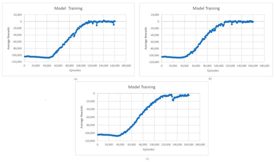
Figure 8.
Learning average rewards for different SoC distribution models: (a) beta distribution; (b) Gaussian distribution; (c) uniform distribution.
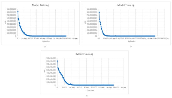
Figure 9.
(a) Learning average loss evolution for different initial SoC distributions: (a) beta distribution; (b) Gaussian distribution; (c) uniform distribution.
In Figure 9, the loss evolution shows the same trend for all three initial SoC distribution models. At first, the loss decreases as the deep Q-learning agent learns, and afterward, it stabilizes. In the case of the Gaussian distribution, stabilization occurs slightly faster than for the other distributions, as the SoC values are more clustered around the mean, providing more consistent training data, which allows the model to learn and reduce loss faster.
For the beta and uniform distributions, the process of loss stabilization in the learning process follows a similar curve. The equal probabilities in the distribution of SoC values foreseen by the uniform distribution led to slower learning rates, as the model must consider a wider range of SoC values. In the case of the beta distribution, the complexity of the learning process is introduced by the fact that initial EVs’ SoC values follow a continuous probability distribution for a fixed interval.
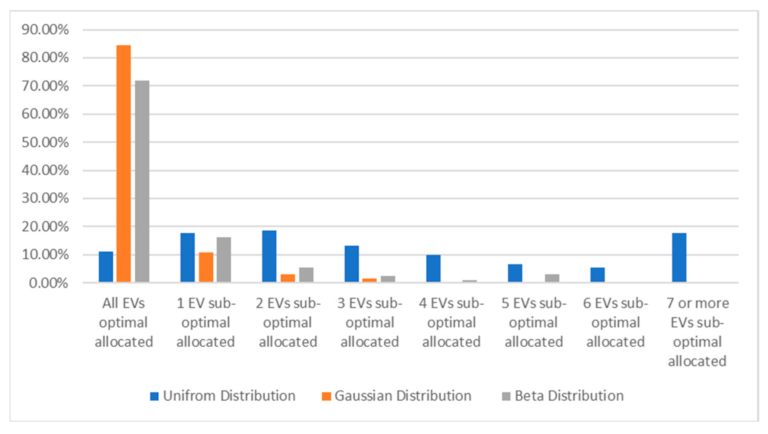
One of their strengths is the ability to learn optimal scheduling policies, in the uncertainty context generated by the small-scale renewable integration. These solutions can adjust to the evolving preferences and behaviors of EV owners, enhancing coordination in the face of uncertainty. Figure 10 presents the percentage of optimal allocations of EVs versus suboptimal ones for the learned policies corresponding to different distributions for EVs’ SoC.
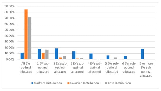
Figure 10.
The percentage of optimal allocations of EVs versus suboptimal ones for beta, Gaussian, and uniform distributions.
This figure indicates that the worst learning performance occurs when the SoC distribution is uniform, a scenario that is not typically encountered in the SoC of a fleet of EVs, as the SoC of vehicle batteries is influenced by various factors and usage patterns, leading to a more diverse and non-uniform distribution.
However, by applying reinforcement learning for a fleet of EV scheduling, there are challenges in dealing with high-dimensional state spaces that make it difficult for the algorithm to converge. High-dimensional states or action spaces can lead to increased computational complexity and difficulties in exploration, which may affect the learning process and hinder convergence. Figure 11 and Figure 12 show the evolution of average rewards and losses in training models for two scenarios with different dimensions of the search space: (i) one featuring a smaller search space, in which we considered 30 cars, 4 charging stations, and a charging interval of 8 h; and (ii) one featuring a bigger search space, in which we considered 30 cars, 8 charging stations, and a charging interval of 4 h. The types of EVs we consider in the two scenarios are those shown in Table 1, and the SoC values of the EVs follow a random distribution.
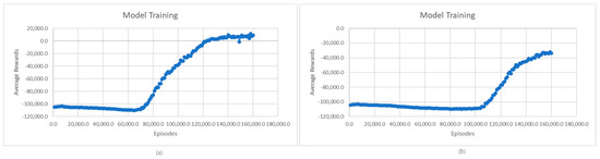
Figure 11.
Average rewards for model training: (a) smaller space scenario; (b) bigger space scenario.
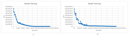
Figure 12.
Average loss for model training: (a) smaller space scenario; (b) bigger space scenario.
In the case of the smaller search space scenario, there is a significant increase in rewards starting at 70,000 episodes, while in the case of the bigger search space scenario, the increase starts at around 110,000 episodes. It is also observed that in the case of the first scenario, a higher average reward value is reached than in the case of the second one. This is because, in the first scenario, with more time slots and fewer charging stations, there is less EV scheduling complexity, which implies a more efficient policy-learning process. The complex scenario requires a longer learning process for policy optimization, achieving lower average reward values.
In the case of the loss evolution shown in Figure 12, the trend is the same for both scenarios. At first, the loss decreases as the models learn, and then, after many episodes, it begins to stabilize. However, in the case of the second scenario, there are small fluctuations as the loss decreases until it reaches stabilization, unlike in the case of the first scenario, where a smoother decrease is registered. This is because in the case of the second scenario, the larger number of charging stations can add higher complexity to the learning process and can influence the balance between exploration and exploitation, leading to fluctuations in losses.
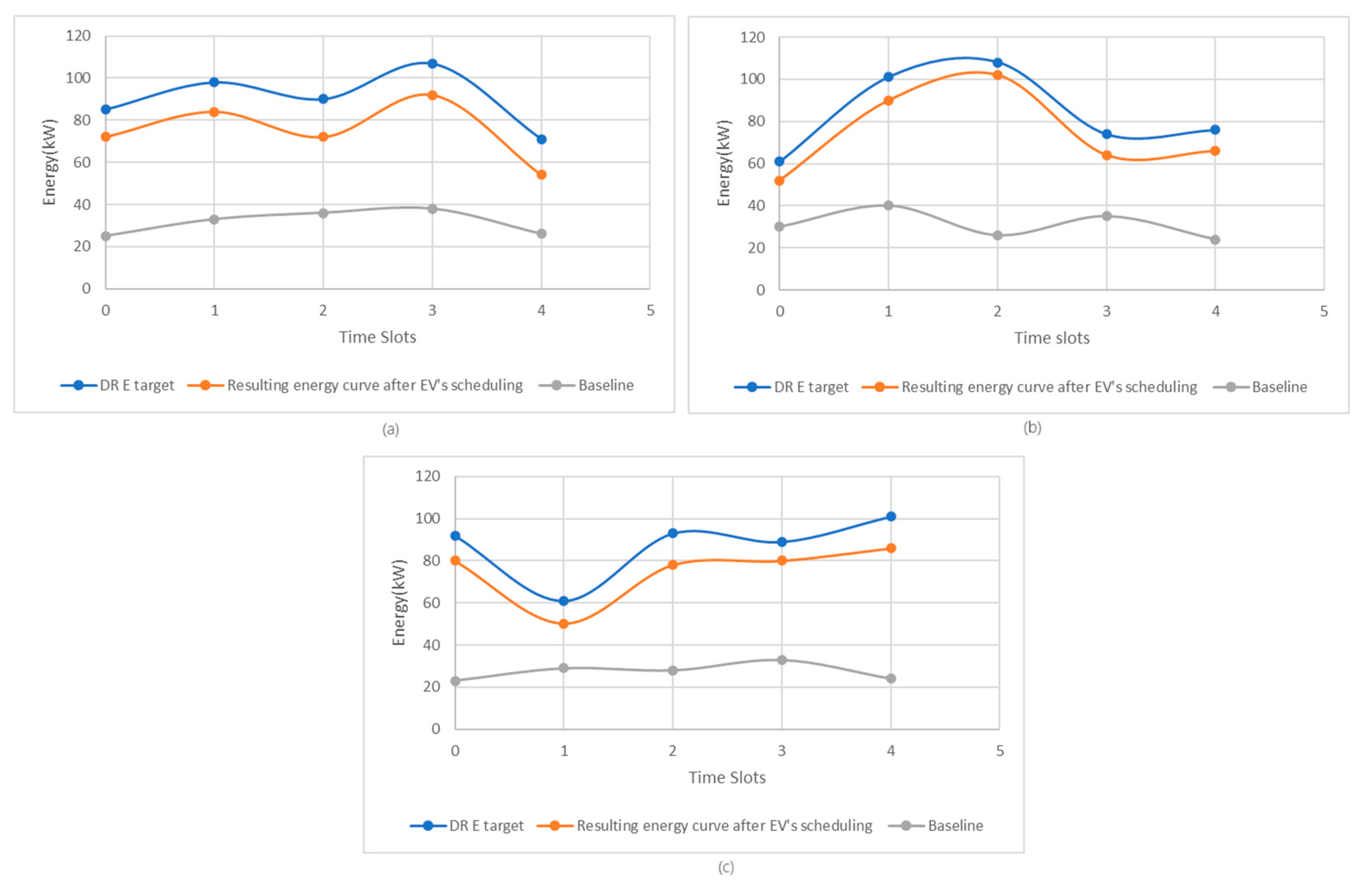
Finally, another notable benefit is that model-free solutions do not necessitate prior knowledge. They dynamically adapt to various scheduling scenarios without relying on a predefined model. Consequently, they are more cost effective compared to model-based solutions, which require specialized knowledge to create and represent the initial optimization framework. Figure 13 shows that our algorithm can generate energy scheduling actions for a fleet of 30 EVs to successfully balance the microgrid’s energy demand and generation. The proposed deep Q-learning algorithm can explore various initial-state configurations for EVs’ state of charge, utilizing different distributions and diverse DR target curves. This exploration is conducted with success without prior knowledge. The scheduled EVs’ energy actions contribute to the achievement of a high degree of similarity between the renewable generation curve and the energy demand curve. This includes the demand of the considered fleet of EVs and the schedules for EVs’ charging output by the algorithm.
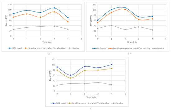
Figure 13.
DR adaptation by scheduling the energy charge of a fleet of EVs using different SoC distributions as the initial state for the learning process: (a) beta distribution, (b) Gaussian distribution, (c) uniform distribution.
6. Conclusions
In this paper, we proposed a deep Q-learning solution for enabling EVs to coordinate and participate in DR programs by scheduling the EVs’ charge and discharge actions to meet a target energy profile. We adapted the Bellman equation to evaluate the EV scheduling state and defined a Q-function to determine the action’s effectiveness in terms of rewards. We represented the Q-function using a neural network to learn from for dynamic EV scheduling scenarios by successively training the available actions and using epsilon-greedy algorithm balances’ exploitation and exploration of the state space.
Our proposed solution offers a promising approach to EV participation in DR programs, which can result in significant benefits for both the distribution system operator and EV owners. The results show that the EVs are scheduled to effectively charge and discharge their collective energy profile to successfully meet the demand requirements’ adaptation in DR programs. Starting from different initial states with different distributions of SoC of EV batteries, the proposed algorithm can learn energy-operational schedules to accurately follow the energy profile provided as a target in DR, with a Pearson coefficient of 0.99. This relives not only the learning algorithm’s effectiveness for a fleet of EVs’ energy management but also its adaptability to different EVs and microgrids without prior configurations and fine-tuning.
In all evaluation cases, the rewards and losses converge to good values, showing the effectiveness of the quality of the learning policy defined for a fleet of EV scheduling as well as of the Q-function in improving the agent’s decision making in the defined microgrid environment. Finally, a limitation of our approach is the fact that the learning process needs a substantial number of episodes to achieve losses and rewards because of the complexity of the environment. There are many states to navigate to gather learning experience due to scheduling combinations of EVs, charging stations, and trade-offs between exploration and exploitation.
As future work, we intend to investigate new EV scheduling solutions by iteratively considering each time slot in the DR program window and not the entire interval, as in the current approach. This type of solution may reduce the number of episodes needed for loss and reward convergence while improving the agent’s responsiveness to changes in the defined EV scheduling environment and promoting greater dynamism in decision making. In addition, we plan to investigate alternative deep Q-learning network architectures to allow the agent to learn and adapt more efficiently with fewer episodes.
Author Contributions
Conceptualization, V.R.C., C.B.P. and T.C.; methodology, T.C. and V.R.C.; formal analysis, V.R.C. and H.G.R.; investigation, I.A. and H.G.R.; resources, I.A.; data curation, H.G.R. and C.B.P.; writing—original draft preparation, V.R.C., T.C., H.G.R. and C.B.P.; writing—review and editing, C.B.P., V.R.C. and I.A.; visualization, H.G.R., I.A. and C.B.P.; project administration, T.C.; funding acquisition, T.C. All authors have read and agreed to the published version of the manuscript.
Funding
This research received funding from the European Union’s Horizon Europe research and innovation program under the Grant Agreement number 101136216. Views and opinions expressed are, however, those of the author(s) only and do not necessarily reflect those of the European Union or the European Climate, Infrastructure, and Environment Executive Agency. Neither the European Union nor the granting authority can be held responsible for them.
Institutional Review Board Statement
Not applicable.
Informed Consent Statement
Not applicable.
Data Availability Statement
The raw data supporting the conclusions of this article will be made available by the authors on request.
Conflicts of Interest
The authors declare no conflicts of interest.
References
- Lou, W.; Chen, Y.; Jin, Y. Energy drive and management of smart grids with high penetration of renewable sources of wind unit and solar panel. Int. J. Electr. Power Energy Syst. 2021, 129, 106846. [Google Scholar]
- Strielkowski, W.; Civín, L.; Tarkhanova, E.; Tvaronavičienė, M.; Petrenko, Y. Renewable Energy in the Sustainable Development of Electrical Power Sector: A Review. Energies 2021, 14, 8240. [Google Scholar] [CrossRef]
- Di Silvestre, M.L.; Favuzza, S.; Sanseverino, E.R.; Zizzo, G. How Decarbonization, Digitalization and Decentralization are changing key power infrastructures. Renew. Sustain. Energy Rev. 2018, 93, 483–498. [Google Scholar] [CrossRef]
- Wu, Y.; Wu, Y.; Guerrero, J.M.; Vasquez, J.C. Digitalization and decentralization driving transactive energy Internet: Key technologies and infrastructures. Int. J. Electr. Power Energy Syst. 2021, 126 Pt A, 106593. [Google Scholar] [CrossRef]
- Li, R.; Satchwell, A.J.; Finn, D. Toke Haunstrup Christensen, Michaël Kummert, Jérôme Le Dréau, Rui Amaral Lopes, Henrik Madsen, Jaume Salom, Gregor Henze, Kim Wittchen, ten questions concerning energy flexibility in buildings. Build. Environ. 2022, 223, 109461. [Google Scholar] [CrossRef]
- Esmat, A.; Usaola, J.; Moreno, M.Á. A Decentralized Local Flexibility Market Considering the Uncertainty of Demand. Energies 2018, 11, 2078. [Google Scholar] [CrossRef]
- Olivella-Rosell, P.; Lloret-Gallego, P.; Munné-Collado, Í.; Villafafila-Robles, R.; Sumper, A.; Ottessen, S.Ø.; Rajasekharan, J.; Bremdal, B.A. Local Flexibility Market Design for Aggregators Providing Multiple Flexibility Services at Distribution Network Level. Energies 2018, 11, 822. [Google Scholar] [CrossRef]
- Kalakanti, A.K.; Rao, S. Computational Challenges and Approaches for Electric Vehicles. ACM Comput. Surv. 2023, 55, 311. [Google Scholar] [CrossRef]
- Khan, S.U.; Mehmood, K.K.; Haider, Z.M.; Rafique, M.K.; Khan, M.O.; Kim, C.-H. Coordination of Multiple Electric Vehicle Aggregators for Peak Shaving and Valley Filling in Distribution Feeders. Energies 2021, 14, 352. [Google Scholar] [CrossRef]
- Liu, G.; Tao, Y.; Xu, L.; Chen, Z.; Qiu, J.; Lai, S. Coordinated management of aggregated electric vehicles and thermostatically controlled loads in hierarchical energy systems. Int. J. Electr. Power Energy Syst. 2021, 131, 107090. [Google Scholar] [CrossRef]
- Venegas, F.G.; Petit, M.; Perez, Y. Active integration of electric vehicles into distribution grids: Barriers and frameworks for flexibility services. Renew. Sustain. Energy Rev. 2021, 145, 111060. [Google Scholar] [CrossRef]
- Needell, Z.; Wei, W.; Trancik, J.E. Strategies for beneficial electric vehicle charging to reduce peak electricity demand and store solar energy. Cell Rep. Phys. Sci. 2023, 4, 101287. [Google Scholar] [CrossRef]
- Jones, C.B.; Vining, W.; Lave, M.; Haines, T.; Neuman, C.; Bennett, J.; Scoffield, D.R. Impact of Electric Vehicle customer response to Time-of-Use rates on distribution power grids. Energy Rep. 2022, 8, 8225–8235. [Google Scholar] [CrossRef]
- Mahmud, I.; Medha, M.B.; Hasanuzzaman, M. Global challenges of electric vehicle charging systems and its future prospects: A review. Res. Transp. Bus. Manag. 2023, 49, 101011. [Google Scholar] [CrossRef]
- Alqahtani, M.; Hu, M. Dynamic energy scheduling and routing of multiple electric vehicles using deep reinforcement learning. Energy 2022, 244 Pt A, 122626. [Google Scholar] [CrossRef]
- Kumar, M.; Panda, K.P.; Naayagi, R.T.; Thakur, R.; Panda, G. Comprehensive Review of Electric Vehicle Technology and Its Impacts: Detailed Investigation of Charging Infrastructure, Power Management, and Control Techniques. Appl. Sci. 2023, 13, 8919. [Google Scholar] [CrossRef]
- Silva, C.; Faria, P.; Barreto, R.; Vale, Z. Fair Management of Vehicle-to-Grid and Demand Response Programs in Local Energy Communities. IEEE Access 2023, 11, 79851–79860. [Google Scholar] [CrossRef]
- Ren, H.; Zhang, A.; Wang, F.; Yan, X.; Li, Y.; Duić, N.; Shafie-khah, M.; Catalão, J.P.S. Optimal scheduling of an EV aggregator for demand response considering triple level benefits of three-parties. Int. J. Electr. Power Energy Syst. 2021, 125, 106447. [Google Scholar] [CrossRef]
- Daina, N.; Sivakumar, A.; Polak, J.W. Modelling electric vehicles use: A survey on the methods. Renew. Sustain. Energy Rev. 2017, 68 Pt 1, 447–460. [Google Scholar]
- Aghajan-Eshkevari, S.; Azad, S.; Nazari-Heris, M.; Ameli, M.T.; Asadi, S. Charging and Discharging of Electric Vehicles in Power Systems: An Updated and Detailed Review of Methods, Control Structures, Objectives, and Optimization Methodologies. Sustainability 2022, 14, 2137. [Google Scholar] [CrossRef]
- Wen, Y.; Fan, P.; Hu, J.; Ke, S.; Wu, F.; Zhu, X. An Optimal Scheduling Strategy of a Microgrid with V2G Based on Deep Q-Learning. Sustainability 2022, 14, 10351. [Google Scholar] [CrossRef]
- Lee, J.; Lee, E.; Kim, J. Electric Vehicle Charging and Discharging Algorithm Based on Reinforcement Learning with Data-Driven Approach in Dynamic Pricing Scheme. Energies 2020, 13, 1950. [Google Scholar] [CrossRef]
- Wan, Z.; Li, H.; He, H.; Prokhorov, D. Model-Free Real-Time EV Charging Scheduling Based on Deep Reinforcement Learning. IEEE Trans. Smart Grid 2019, 10, 5246–5257. [Google Scholar] [CrossRef]
- Viziteu, A.; Furtună, D.; Robu, A.; Senocico, S.; Cioată, P.; Remus Baltariu, M.; Filote, C.; Răboacă, M.S. Smart Scheduling of Electric Vehicles Based on Reinforcement Learning. Sensors 2022, 22, 3718. [Google Scholar] [CrossRef] [PubMed]
- Cao, Y.; Wang, Y. Smart Carbon Emission Scheduling for Electric Vehicles via Reinforcement Learning under Carbon Peak Target. Sustainability 2022, 14, 12608. [Google Scholar] [CrossRef]
- Liu, D.; Zeng, P.; Cui, S.; Song, C. Deep Reinforcement Learning for Charging Scheduling of Electric Vehicles Considering Distribution Network Voltage Stability. Sensors 2023, 23, 1618. [Google Scholar] [CrossRef] [PubMed]
- Paraskevas, A.; Aletras, D.; Chrysopoulos, A.; Marinopoulos, A.; Doukas, D.I. Optimal Management for EV Charging Stations: A Win–Win Strategy for Different Stakeholders Using Constrained Deep Q-Learning. Energies 2022, 15, 2323. [Google Scholar] [CrossRef]
- Wang, R.; Chen, Z.; Xing, Q.; Zhang, Z.; Zhang, T. A Modified Rainbow-Based Deep Reinforcement Learning Method for Optimal Scheduling of Charging Station. Sustainability 2022, 14, 1884. [Google Scholar] [CrossRef]
- Li, H.; Wan, Z.; He, H. Constrained EV Charging Scheduling Based on Safe Deep Reinforcement Learning. IEEE Trans. Smart Grid 2020, 11, 2427–2439. [Google Scholar] [CrossRef]
- Cui, F.; Lin, X.; Zhang, R.; Yang, Q. Multi-objective optimal scheduling of charging stations based on deep reinforcement learning. Front. Energy Res. 2023, 10, 1042882. [Google Scholar] [CrossRef]
- Heendeniya, C.B.; Nespoli, L. A stochastic deep reinforcement learning agent for grid-friendly electric vehicle charging management. Energy Inform. 2022, 5 (Suppl. S1), 28. [Google Scholar] [CrossRef]
- Shi, J.; Gao, Y.; Wang, W.; Yu, N.; Ioannou, P.A. Operating Electric Vehicle Fleet for Ride-Hailing Services with Reinforcement Learning. IEEE Trans. Intell. Transp. Syst. 2020, 21, 4822–4834. [Google Scholar] [CrossRef]
- Li, S.; Hu, W.; Cao, D.; Dragicevic, T.; Huang, Q.; Chen, Z.; Blaabjerg, F. Electric Vehicle Charging Management Based on Deep Reinforcement Learning. J. Mod. Power Syst. Clean. Energy 2022, 10, 719–730. [Google Scholar] [CrossRef]
- Ding, T.; Zeng, Z.; Bai, J.; Qin, B.; Yang, Y.; Shahidehpour, M. Optimal Electric Vehicle Charging Strategy with Markov Decision Process and Reinforcement Learning Technique. IEEE Trans. Ind. Appl. 2020, 56, 5811–5823. [Google Scholar] [CrossRef]
- Park, K.; Moon, I. Multi-agent deep reinforcement learning approach for EV charging scheduling in a smart grid. Appl. Energy 2022, 328, 20111. [Google Scholar] [CrossRef]
- Mohanty, S.; Panda, S.; Parida, S.M.; Rout, P.K.; Sahu, B.K.; Bajaj, M.; Zawbaa, H.M.; Kumar, N.M.; Kamel, S. Demand side management of electric vehicles in smart grids: A survey on strategies, challenges, modeling, and optimization. Energy Rep. 2022, 8, 12466–12490. [Google Scholar] [CrossRef]
- Vishnu, G.; Kaliyaperumal, D.; Jayaprakash, R.; Karthick, A.; Kumar Chinnaiyan, V.; Ghosh, A. Review of Challenges and Opportunities in the Integration of Electric Vehicles to the Grid. World Electr. Veh. J. 2023, 14, 259. [Google Scholar] [CrossRef]
- Mignon, A.D.S.; de Azevedo da Rocha, R.L. An Adaptive Implementation of ε-Greedy in Reinforcement Learning. Procedia Comput. Sci. 2017, 109, 1146–1151. [Google Scholar] [CrossRef]


Disclaimer/Publisher’s Note: The statements, opinions and data contained in all publications are solely those of the individual author(s) and contributor(s) and not of MDPI and/or the editor(s). MDPI and/or the editor(s) disclaim responsibility for any injury to people or property resulting from any ideas, methods, instructions or products referred to in the content. |
© 2024 by the authors. Licensee MDPI, Basel, Switzerland. This article is an open access article distributed under the terms and conditions of the Creative Commons Attribution (CC BY) license (https://creativecommons.org/licenses/by/4.0/).