Greenhouse Ventilation Equipment Monitoring for Edge Computing

Abstract

Digital twins based on real-world scenarios are heavily reliant on extensive on-site data, representing a significant investment in information technology. This study aims to maximize the capabilities of visual sensors, like cameras in controlled-environment agriculture, by acquiring more target-specific information at minimal additional cost. This approach not only reduces investment but also increases the utilization rate of existing equipment. Utilizing YOLOv7, this paper introduces a system with rotatable pan-tilt cameras for the comprehensive monitoring of large-scale greenhouse ventilation systems. To mitigate the computational load on edge servers at greenhouse sites caused by an abundance of video-processing tasks, a Region of Interest (ROI) extraction method based on tracking is adopted. This method avoids unnecessary calculations in non-essential areas. Additionally, we integrate a self-encoding approach into the training phase, combining object detection and embedding to eliminate redundant feature extraction processes. Experimental results indicate that ROI extraction significantly reduces the overall inference time by more than 50%, and by employing LSTM to classify the state of the fan embedding sequences, a 100% accuracy rate was achieved.

1. Introduction

Facility agriculture, a cornerstone of modern agriculture [1], aims to create a controlled artificial environment for crops, providing essential growth conditions such as temperature, light, fertilization, and gases. Greenhouses represent a contemporary production approach that amalgamates engineering, biotechnology, and environmental technology to optimize the environment for the growth and development of flora and fauna. Research into greenhouse equipment monitoring is pivotal for remote environmental adjustments and facilitating the development of digital twin systems [2]. Current greenhouse monitoring systems primarily focus on internal environmental conditions and crop growth, often overlooking the operational status of the equipment within [3].

Traditional approaches to monitoring equipment rely heavily on specific sensors to track operational status [4]. These methods are costly in terms of installation and maintenance, and their lifespan and stability are susceptible to environmental factors. To address these issues, Qin et al. [5] employed video surveillance for the remote monitoring of greenhouse ventilation, circumventing the need for specialized sensors. This technique utilizes the frame difference method and autocorrelation function methods to assess the operational status of fans. However, it requires fixed-angle cameras and is sensitive to background changes, making it less suitable for pan-tilt cameras with variable viewing angles. To overcome these limitations and maximize the potential of pan-tilt cameras, we have incorporated deep learning techniques to develop a versatile method for detecting equipment and recognizing its status.

In the application of deep learning for equipment state recognition, the process typically involves dividing the task into two distinct phases [6]: object detection and state recognition. Initially, object detection techniques identify objects within an image, followed by the utilization of an image classification network to recognize the status of these detected objects. For instance, Lao et al. [7] employed YOLOv5 for bolt detection in images and PIPNet to detect key points for assessing bolt status and identifying defects. While utilizing deep learning in both phases enhances accuracy and generalizability, it demands considerable computational resources. This poses challenges in achieving optimal performance on edge computing [8,9] devices, such as the RK3399Pro platform discussed in this study.

In recent years, a significant body of research has developed which focuses on enhancing real-time object detection or its integration with other tasks. These studies aim to optimize the balance between detection efficiency and precision within the constraints of limited resources. Object detection methodologies are principally categorized into two-stage networks, exemplified by Faster R-CNN, and one-stage networks, typified by YOLO. The pursuit of real-time capabilities predominantly employs one-stage networks. The strategies employed to augment detection speed are varied, encompassing the adoption of lighter network architectures, the implementation of multi-task learning for multiple tasks, and the design of more straightforward features. Zheng et al. [10] conducted a comparative analysis of object detection networks within the context of forest smoke detection, discovering that YOLOv3 delivers the most rapid detection alongside commendably high precision. To address the inefficiencies of Non-Maximum Suppression (NMS) in one-stage methodologies, Sun et al. [11] introduced an innovative end-to-end detection algorithm that obviates the need for NMS. By redefining the loss function, treating the instance with minimal loss as the positive sample (and all others as negative), and selecting the top k results in the post-processing phase, they refined the training process. Lai et al. [12] embarked on research into pedestrian detection and action recognition on Unmanned Aerial Vehicles (UAVs) and designed a model that jointly trains two tasks to achieve the transfer of deep features. Their methodology initiates with the detection of pedestrians through an object detection network, followed by the extraction of deep feature maps for the integration of temporal data, using BNLSTM for action detection. Zheng et al. [13], in the context of autonomous driving, added multiple output heads to a network to simultaneously perform traffic object detection, drivable area segmentation, and lane detection, with adjustments to the network’s architecture and loss functions tailored to maintain precision.

In order to accommodate resource constraints in edge computing scenarios, the demand for high detection speed and accuracy when processing real-time video streams, and the limitations of computing platforms for operators, such as the lack of support for ROI-align, etc., our research is based on YOLOV7-tiny. We integrated the object detection functionality of YOLOv7 [14] with the feature extraction capabilities of autoencoders [15] to enable the use of simple sequential classification models such as LSTM to effectively identify the state of equipment. Furthermore, acknowledging the sequential nature of video images, we propose a method for extracting regions of interest based on object tracking. This method effectively reduces computational load by excluding irrelevant areas, thus conserving computational resources.

2. Methods

2.1. Related Works

YOLOv7 exemplifies an advanced end-to-end object detection paradigm. It eschews the complexities inherent in multi-stage detection frameworks by delivering target detection in a singular computational stride. This model parses an input image into a grid-based schema, within which it prognosticates bounding boxes and class probabilities for each grid cell, thereby furnishing rapid and precise target detection in real-time contexts. The YOLOv7 network is composed of three sections: a backbone network for feature extraction, a neck network for feature integration, and an output layer for generating detection predictions. Beginning with an RGB image, the backbone network processes the image through several convolution and pooling steps. This processing progressively reduces the feature map’s resolution and increases its depth to extract richer semantic information. The network’s neck section further enhances these feature maps by integrating them across different layers, expanding the network’s ability to perceive various scales. Detection predictions are made in the final stage, with each cell of the network proposing three candidate detections based on predefined anchor points. As illustrated in Figure 1, an input image with dimensions of 1280 × 1280 will have its feature map resolution reduced in the backbone network progressively (by 2×, 4×, 8×, 16×, and 32×) to 40 × 40. After passing through the neck network, the output layer will receive (40 × 40 + 80 × 80 + 160 × 160) × 3 candidate targets. The final detection results require the use of non-maximum suppression to filter similar candidate boxes.

In the domain of unsupervised learning, autoencoders have been seminal, enabling feature learning and data compression by distilling input data into a more compact, informative embedding. The autoencoder architecture bifurcates into an encoder, which condenses the input data (e.g., images) into a lower-dimensional space, and a decoder, which endeavors to reconstruct the input from this compressed embedding. This process of data compression and reconstruction allows the encoder to capture and retain the fundamental features and semantic essence of the input, thus ensuring that the integrity of the original data is largely preserved within the reduced embedding space. As illustrated in Figure 2, the encoder and decoder are trained to minimize the discrepancy between the encoder input and the decoder output, enabling the encoder to efficiently compress high-dimensional data into a low-dimensional space.

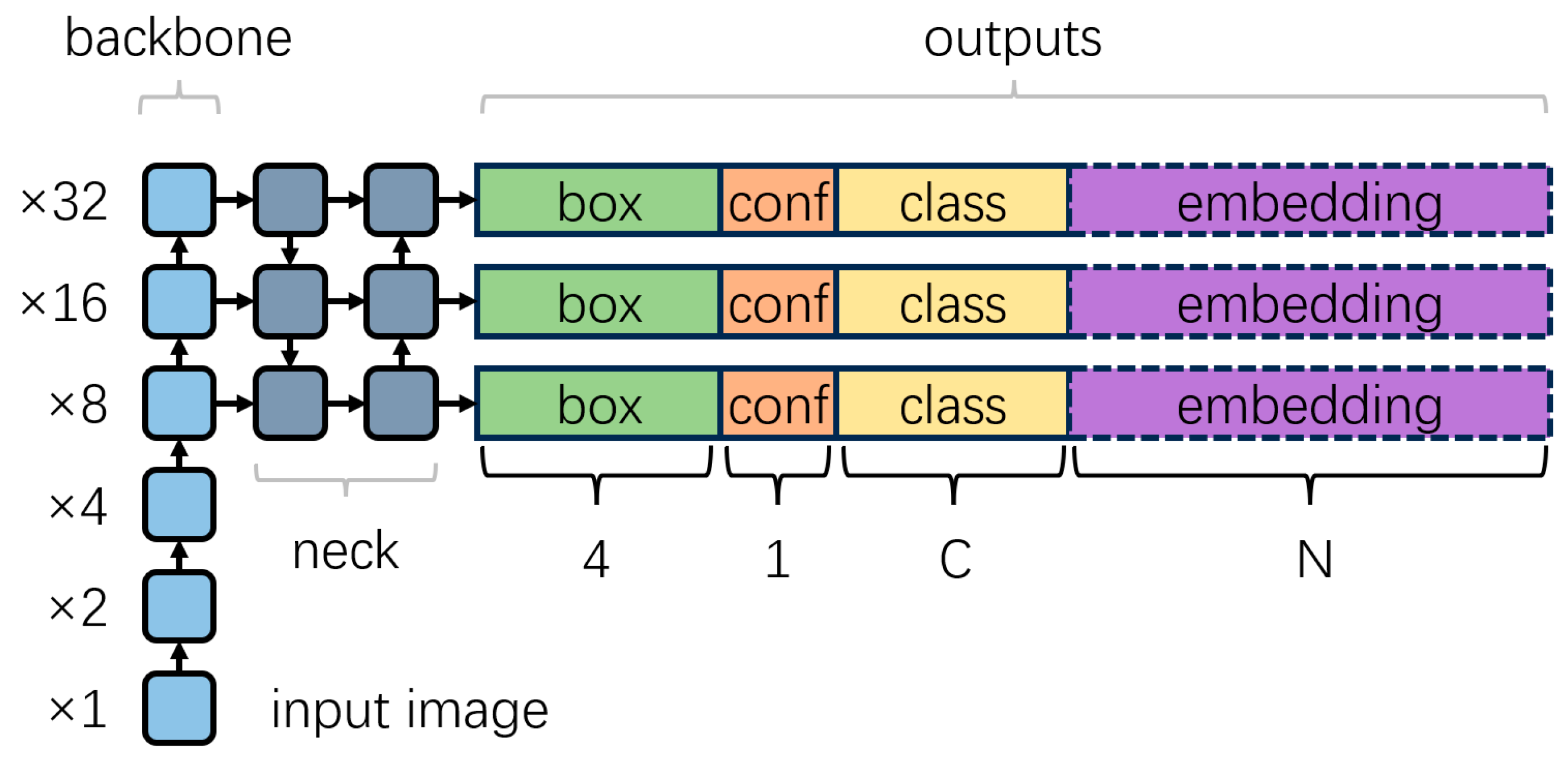
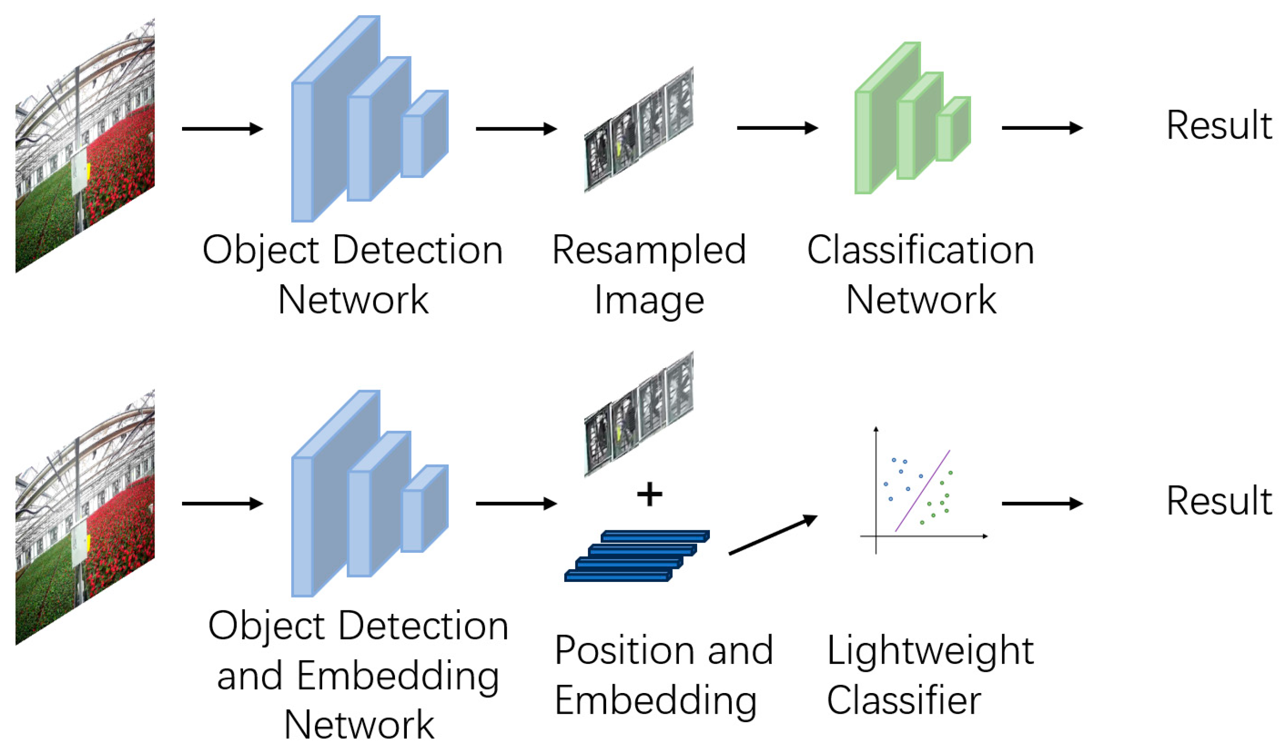
2.2. Integration of Detection and Embedding

In computational tasks in which concurrent object detection and state recognition is a requisite, conventional methodologies typically necessitate a resampling of the original image after the detection phase, followed by the application of specialized algorithms for state recognition, as shown in Figure 3. Our integrated approach seeks to streamline this process by encapsulating both detection and embedding functionalities within a singular forward pass of the network. This strategy leverages a low-dimensional embedding of the target image, which serves as a distilled representational form, facilitating the extraction of state information with significantly reduced computational demands. We opted for the YOLOv7 model as an object detection network. Among various object detection methods, the YOLO series is widely recognized for its detection speed. YOLOv7, as one of the newer iterations, incorporates many advantages from previous research, making it a comprehensive solution for real-time applications. Specifically, YOLOv7-tiny, a variant with significantly fewer parameters (only 6.2 M), has been proven effective. It strikes an excellent balance between detection speed and detection accuracy, making it highly suitable for edge computing environments in which resources are limited. Concurrently, we incorporated an autoencoder into the YOLOv7 training regimen to imbue it with the requisite capabilities for target embedding.

To empower YOLOv7 with the functionality to output an embedding reflective of the target’s state, we expanded the channel capacity of the output layer, which shown in Figure 2. This modification enables each grid cell to maintain its primary detection output while appending a state embedding vector. Consequently, each candidate target within the grid is represented by a comprehensive output ensemble that includes central coordinates, dimensions, a confidence score, class probabilities, and a state embedding vector. This state embedding vector, characterized by a predetermined length, encapsulates the salient attributes of the target’s state.

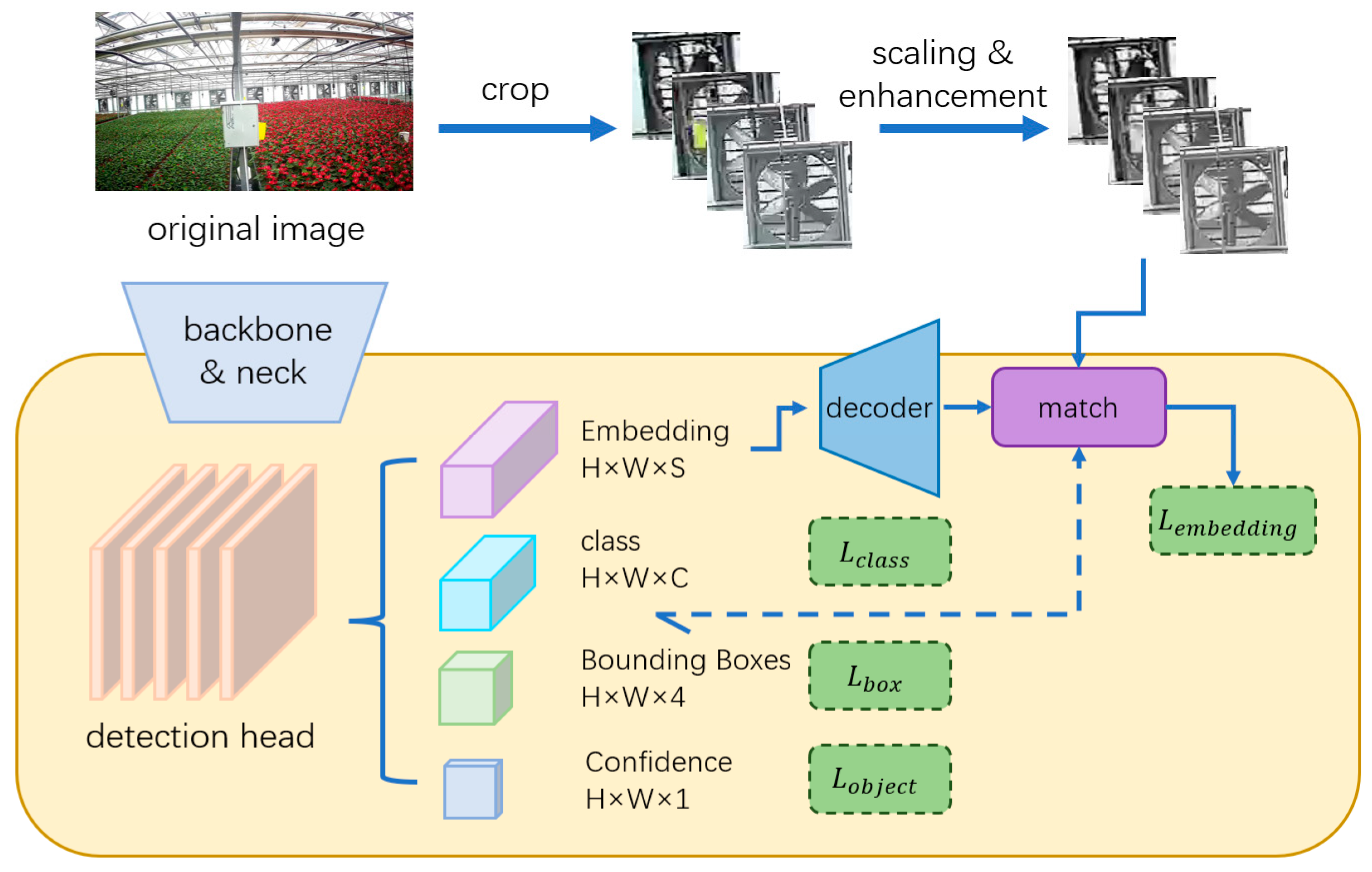
2.2.1. Integration Method

We used a decoder in training to guide YOLOv7 to generate meaningful state embeddings rather than direct embedding learning. These tasks aid networks in developing features beneficial to the main objective. Illustrated in Figure 4, the decoder of an image autoencoder reconstructs the target’s state embedding back into its original image or a variant. Reducing the disparity between the target image and its autoencoder reconstruction ensures that the state embedding encompasses the target’s visual features. During training strategy’s forward propagation, the detection module first ascertains the candidate target’s confidence, dimensions, classification, and state embedding, which the decoder then transforms back into an image representation.

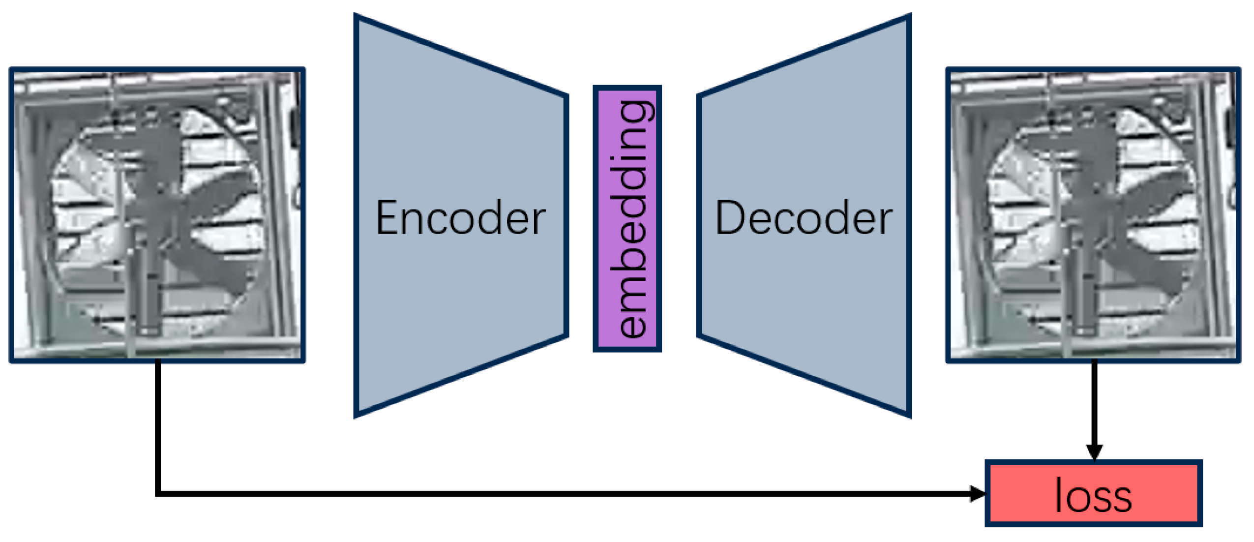
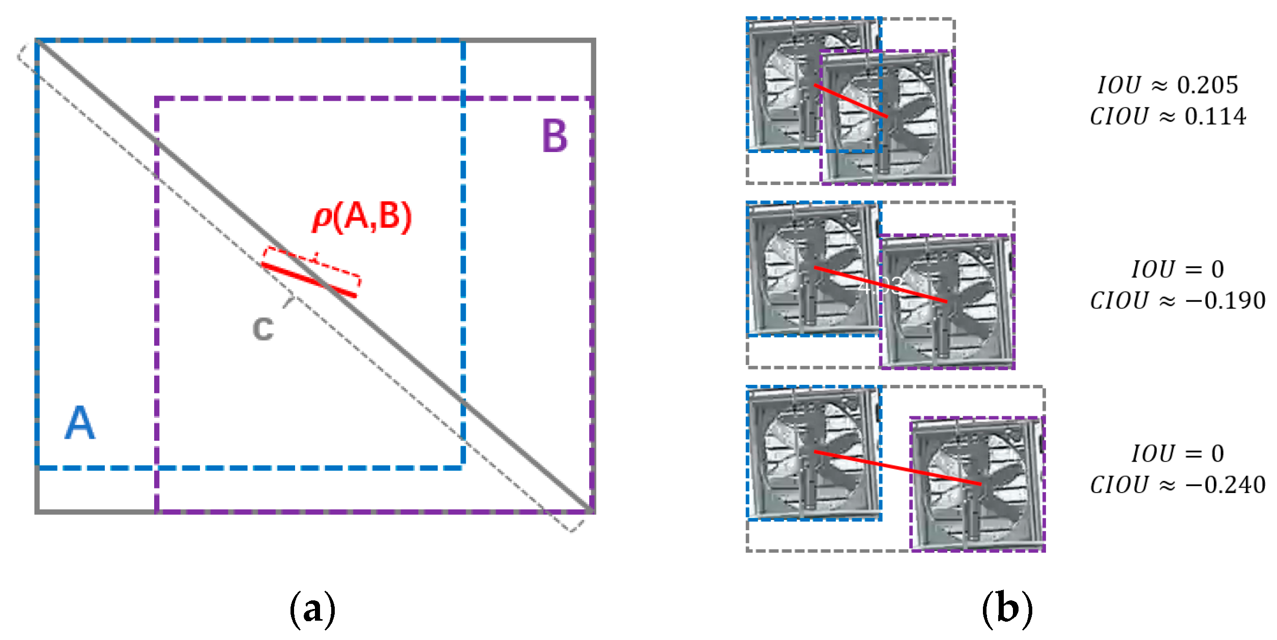
2.2.2. Loss Function

Mirroring YOLOv7, our model’s loss function is multifaceted, optimizing both detection and state embedding. For state embedding, reconstruction loss is introduced, employing L1 loss to gauge the disparity between the decoder’s output and the actual target image. The model’s overall loss is a weighted average of confidence, dimension, classification, and reconstruction losses.

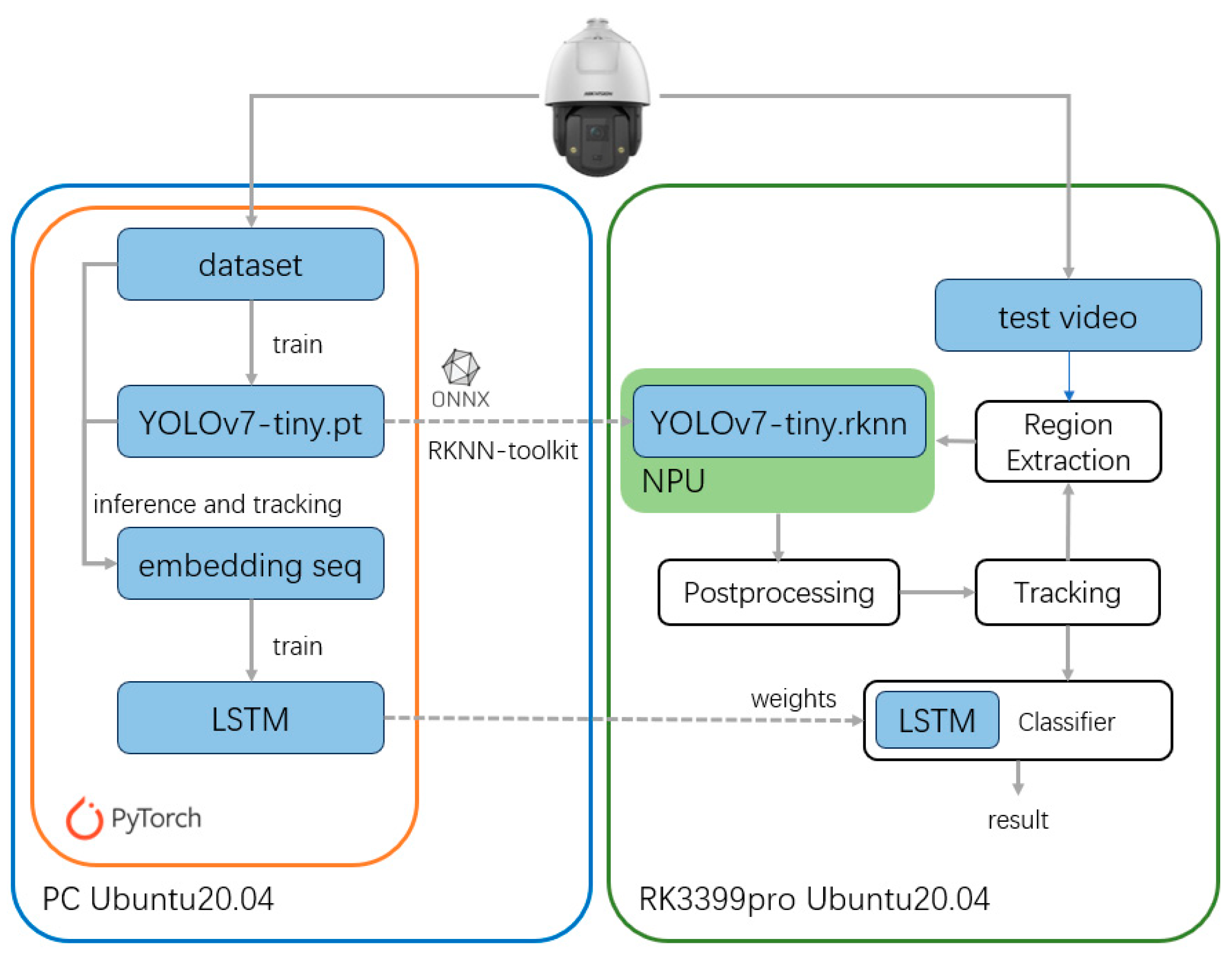
2.2.3. Training Methodology

The training strategy used profoundly impacts the final performance of our model. A key aspect of our approach is the synergistic training of the detection and decoder components to establish effective mapping between the target embedding and the state representation. To achieve this, the target embedding output by the detection head must be precisely matched with the actual targets.

Our alignment process involves matching the bounding boxes proposed by the detection head with the ground truth bounding boxes. This matching is critical to ensuring that the state embeddings are representative of the actual target features. To refine this process, we employ the Complete Intersection over Union [16] (CIoU) metric, which considers the overlap between predicted and actual bounding boxes along with additional factors like aspect ratio and central point distance to provide a more holistic measure of the detection accuracy.

Targets with a CIoU below a certain threshold are excluded to maintain the integrity of the matching process. This filtration step is essential to enhance the precision of target matching as it ensures that only bounding boxes with a high degree of overlap and geometric congruence are considered. This selective consideration allows the model to learn from the most accurate predictions, reinforcing the encoder’s ability to generate high-fidelity state embeddings.

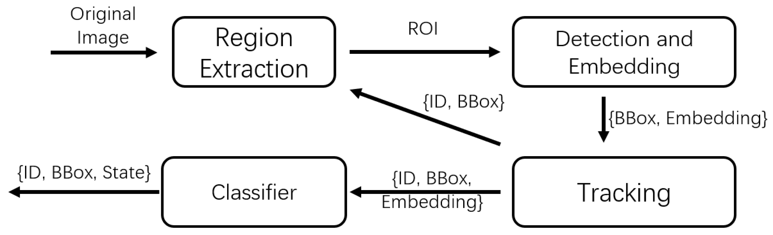
2.3. Extracting Regions of Interest Based on Tracking

In surveillance scenarios, as depicted in Figure 5, the targets usually occupy a minimal portion of the visual field. Processing the entire image for detection purposes incurs significant computational resource expenditure. Consequently, focusing on regions of interest within the image for detection can substantially mitigate computational demands when employing deep learning algorithms for target detection.

Methods for region extraction are categorized into two main approaches: those that employ deep learning techniques [17] and those that do not [18,19]. Deep learning-based approaches are characterized by their high accuracy and ability to interpret scene content, albeit at the cost of significant computational resources. Alternatively, methods such as optical flow, edge detection, and template matching are employed for region extraction in a more resource-efficient manner. These techniques, however, necessitate the manual identification of certain features to generate region proposals. Given the frequent need for target tracking in continuous video frames within systems, employing such methodologies for the predictive positioning of targets in subsequent frames proves advantageous. By centering multiple rectangles on the predicted centers of identified objects, these methods effectively encapsulate areas of interest without imposing additional computational demands.

The method’s data flow, as illustrated in Figure 6, is depicted as follows: initially, the region extractor, utilizing the preceding frame’s object tracking predictions, isolates images containing the object. Subsequently, a modified YOLOv7 algorithm detects each region, with the outputs amalgamated for comprehensive post-processing. Object tracking then correlates targets across frames, forecasting future positions to inform region extraction. The final step involves a classifier discerning the object’s state from its embedding. In our context, fans exhibit two states: active and inactive. Experimental results demonstrate that the LSTM classifier suffices for accurate categorizations of state.

For the target-tracking aspect, our approach refers to the SORT algorithm [20], employing Kalman filtering and Intersection over Union (IOU) matching for efficient tracking. SORT, renowned for its real-time performance and simplicity, is pivotal in multi-target-tracking scenarios. Its core principle revolves around utilizing Kalman filtering for modeling target velocity and position in video frames, followed by the application of the Hungarian algorithm to align predicted and detected values in subsequent frames. This methodology excels in minimizing mismatch errors and is characterized by low computational complexity, rendering it ideal for real-time applications. In our study, we utilize IoU-based matching, aligning positions and sizes predicted by the Kalman filter with those determined by the target detector.

In our experiment, Kalman filtering accomplishes tracking by establishing a 6-dimensional state vector which includes the center coordinates (x, y), the dimensions (width, height) of the bounding box, and the velocity of center coordinate changes (Δx, Δy). This form allows for an effective representation of the target’s dynamics, not just capturing its spatial positioning but also incorporating its movement speed, facilitating precise target tracking through sequential video frames. At the start of a tracking algorithm loop, the algorithm updates this vector using the state transition matrix to predict the positions of targets at that moment, in our case, by adding the last two dimensions to the first two dimensions. Subsequently, targets in consecutive frames are matched based on the CIoU. Finally, the state vector is updated using the matching results according to the Kalman filter’s state update equation.

Considering the relative stability of target aspect ratios in consecutive video frames captured by cameras, we utilize the CIOU metric. An enhanced version of IOU, CIOU not only accounts for the aspect ratios and centroid distances of bounding boxes but also circumvents tracking loss scenarios which are typical when IOU values approach zero. As Figure 7 demonstrates, in instances in which consecutive frames lack target overlap, resulting in an IOU of zero, CIOU effectively measures the centroids’ proximity and shape resemblance, thereby facilitating more accurate matching.

The CIOU formula is expressed as follows:

$$IOU=\frac{A\cap B}{A\cup B}$$

(1)

$$CIOU=IOU-\frac{{\rho }^2\left(A,B\right)}{c^2}-\alpha v$$

(2)

$$\alpha =\frac{v}{\left(1-IOU\right)+v}$$

(3)

$$v=\frac{4}{{\pi }^2}{({\tan }^{-1}\frac{w^A}{h^A}-{\tan }^{-1}\frac{w^B}{h^B})}^2$$

(4)

A and B symbolize the target bounding boxes across consecutive frames, $\rho \left(A,B\right)$ represents the Euclidean distance between their centroids, and $c$ denotes the diagonal length of their minimal enclosing area. CIOU integrates IOU with two penalization terms: the first, $\frac{{\rho }^2\left(A,B\right)}{c^2}$, quantifies the centroids’ distance (0 when coinciding; 1 at a maximum distance); the second, $\alpha v$, evaluates the bounding boxes’ shape similarity. Among them, the $v$ value increases with widening aspect ratio disparities, and $\alpha$, a balancing factor, amplifies in conjunction with rising IOU values, keeping $v$ constant.

3. Experiments

3.1. Experimental Configuration

As shown in Figure 8, this study comprises two main experimental sections. Model training was executed on an Ubuntu 20.04 system equipped with an i9-11900k CPU (Intel, Santa Clara, CA, USA) and NVIDIA GTX 3090 GPU (NVIDIA, Santa Clara, CA, USA), boasting 24 G of video memory. The modified YOLOv7-tiny was developed using the Pytorch framework, compatible with CUDA version 11.3. Detection speed was assessed on edge computing devices, specifically on the RK3399Pro platform with Ubuntu 20.04, utilizing RKNPU for YOLOv7’s network inference (RKNN version 1.7.3). The RK3399Pro, developed by Rockchip (Fuzhou, China), is an embedded development board designed for applications in embedded deep learning fields such as intelligent driving, security monitoring, and robotics. It features a multi-core CPU based on ARM architecture, including the Cortex-A72 and Cortex-A53 (Intel, Santa Clara, CA, USA) cores in a big.LITTLE architecture, with a maximum CPU frequency of 1.8 GHz. In addition to the CPU, the RK3399Pro is equipped with Rockchip’s proprietary second-generation embedded RK NPU (Neural Processing Unit) architecture, which operates at a peak frequency of 700 MHz and offers a computational power of up to 3 TOPS. The RKNPU shares 4 GB LPDDR3 memory with the CPU, optimizing the board’s performance in handling AI tasks and making it an ideal choice for edge computing applications that require efficient processing and AI capabilities.

The dataset originates from surveillance footage within the Shanghai Yingmiao Fruits and Vegetables Professional Cooperative’s greenhouse, obtained from a position on upper crossbeams. Targets in the videos were annotated using CVAT and exported as images for model training. It encompasses three surveillance sequences: the first two show stationary camera angles capturing varied scenarios like fans in different operational states and spray mist interference. The third sequence features horizontal camera rotation to enhance the variety of fan samples and to test detection capabilities during motion. In total, 417 images from these sequences were utilized for training.

3.2. Training of Object Detection and Embedding Model

The experiment employed the YOLOv7-tiny model, modified to output feature embeddings by increasing the parameter count for each potential target in the IDetect layer. The changes are as follows:

$$N_{output}=5+nc$$

(5)

$${N^{\prime }}_{output}=5+nc+ne$$

(6)

$N_{output}$ denotes the parameter count output per anchor in each grid, with nc as the category count and ne as the feature vector width. In this case, ne was chosen to be 64, indicating the length of each feature vector.

The model’s decoder comprises two deconvolution blocks and a fully connected layer. The fully connected layer transforms a 64-dimensional embedding into a 1616 feature map, which is then expanded to 64 × 64 by two deconvolution blocks. Each deconvolution block contains three units, each comprising deconvolution layer, batch normalization, and an activation function. Finally, the decoder outputs a reconstructed image after passing through a convolution layer and a sigmoid activation function.

Model training was conducted using the Stochastic Gradient Descent (SGD) optimizer to mitigate overfitting in scenarios with limited samples. The OneCycleLR learning rate scheduler was implemented to expedite model convergence. The batch size was 16, and a total of 300 epochs were trained. The input size is 1280 × 1280.

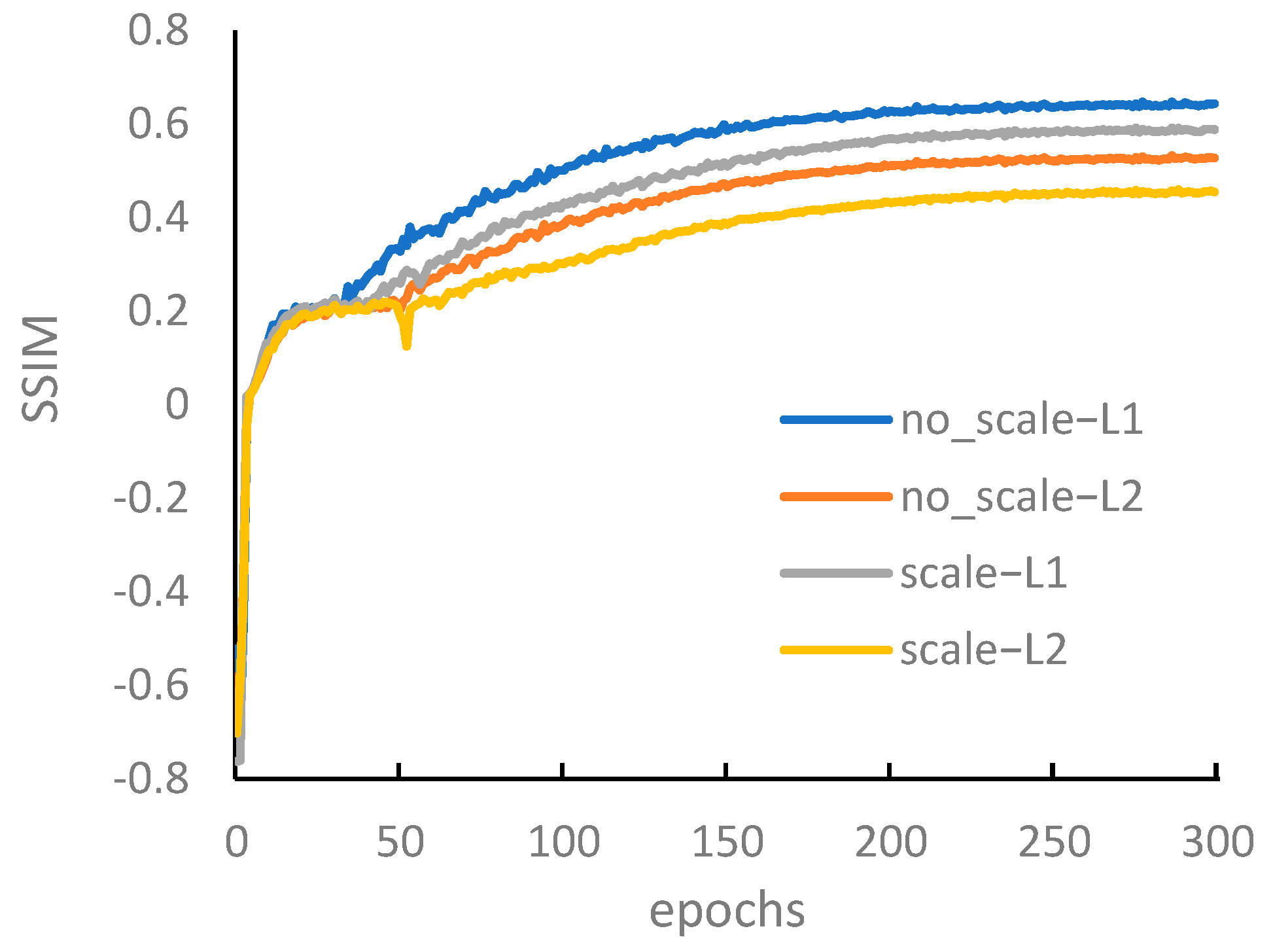
3.2.1. Image Reconstruction Losses

The efficacy of image reconstruction serves as an indicator of a model’s ability to encode states. A superior image reconstruction quality implies a richer representation of target image information within the embedding. This study predominantly focuses on L2 and L1 losses, omitting PSNR due to its strong correlation with L2. This research adopts the SSIM [21] for evaluating the similarity between reconstructed and original images. SSIM diverges from traditional pixel-based quality assessments by prioritizing changes in image structure measured through luminance, contrast, and structure. The SSIM value, ranging from −1 to 1, signifies similarity, with values closer to 1 indicating greater resemblance. The SSIM is computed as follows:

$$SSIM\left(A,B\right)=\frac{(2{\mu }_A{\mu }_B+C_1)(2{\sigma }_{AB}+C_2)}{({\mu }_A^2{+\mu }_B^2+C_1)({\sigma }_A^2+{\sigma }_B^2+C_2)}$$

(7)

where A and B represent two images for comparison, ${\mu }_A$ and ${\mu }_B$ denote their mean luminance values, ${\sigma }_A^2$ and ${\sigma }_B^2$ their variances, ${\sigma }_{AB}$ Is the covariance, and $C_1$ and $C_2$ are constants to stabilize the denominator.

As shown in Figure 9, this experiment shows that L1 loss facilitates superior image reconstruction, outperforming L2 loss, regardless of the employment of image scaling as a data augmentation technique. Furthermore, the models demonstrated enhanced capability in reconstructing target images without the utilization of image scaling during training.

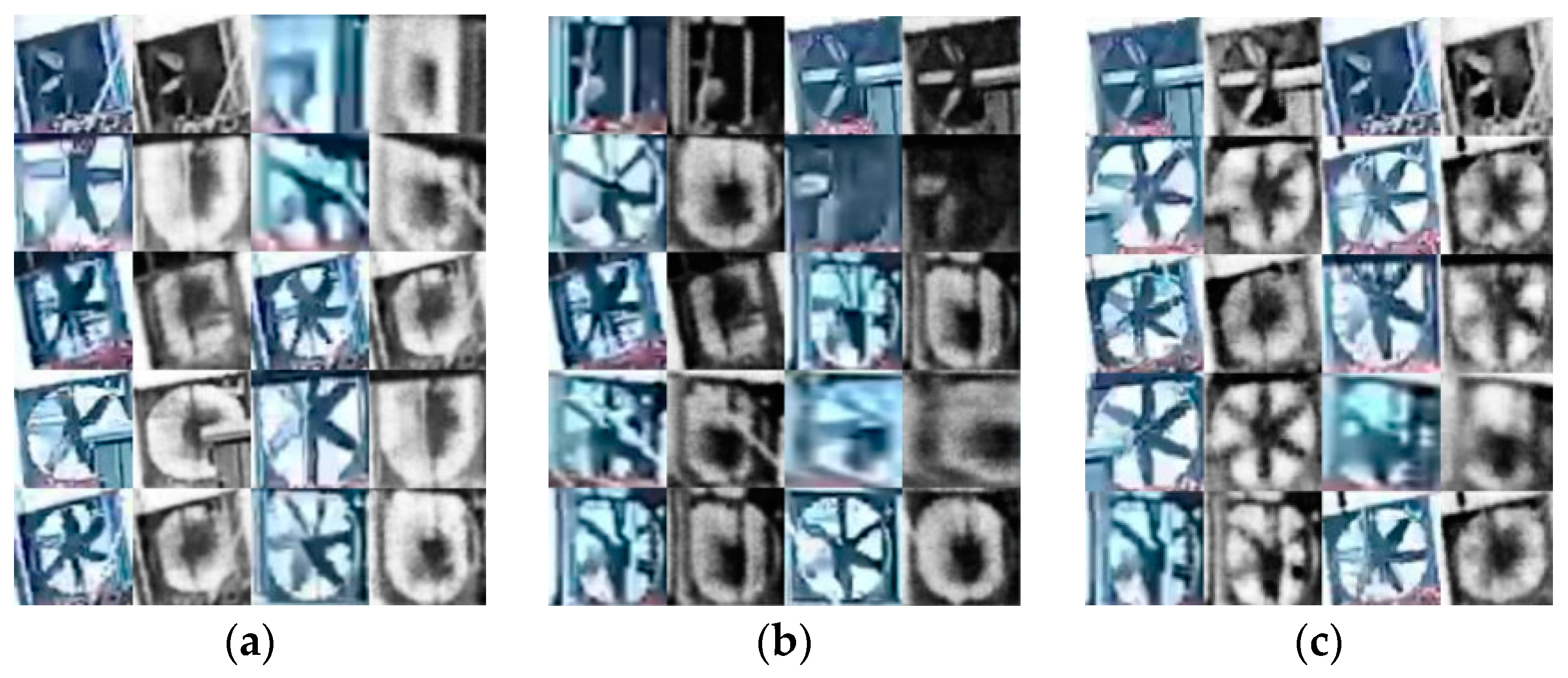
3.2.2. Influence of Various Image Enhancement Techniques

This study demonstrates that without applying enhancement techniques to the original images, achieving accurate representations of targets in reconstructed images remains a challenge. This discrepancy primarily arises due to significant variations in the appearance of images under diverse lighting conditions, even for identical target states. To address this issue, we evaluated three distinct image enhancement strategies: normalization, gamma transformation, and histogram equalization.

As shown in Figure 10, histogram equalization markedly surpasses alternative methods in enhancing the visibility of critical details in reconstructed images, such as the blades of fans. Comparing the enhanced images, the reason may be that it is difficult to effectively distinguish details in images processed by other means except for histogram equalization. Inadequate representations of these blades in reconstructed images could significantly impede the accurate analysis of their rotation.

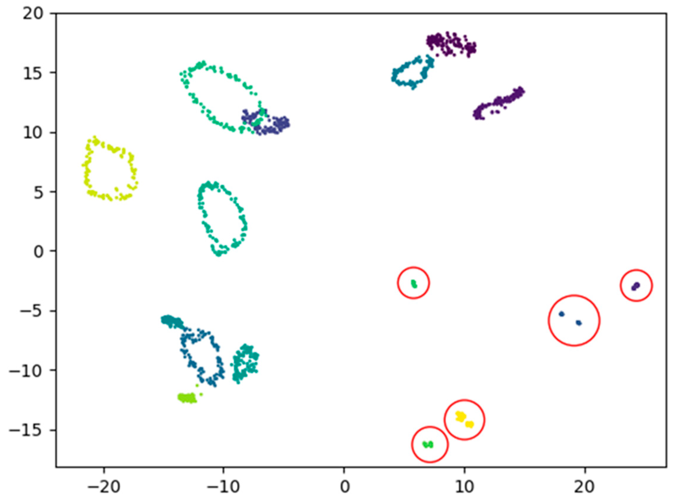
3.2.3. Fan State Recognition

To assess the validity of state embedding for fans, we classified their states based on these embeddings. In our study, we analyzed fans within the same segment of video footage, detecting and embedding a state sequence for 16 fans, each with a length of 117, corresponding to the frame count of the video segment. The distribution of these sequences, followed a dimensionality reduction via a Principal Component Analysis (PCA) [22].

Figure 11 illustrates clusters in which each color-coded point signifies the coordinates of fans in various frames post-PCA reduction. Fans not in operation are encircled in red. These clusters demonstrate distinct groupings that may be influenced by varying angles of capture, leading to differing distributions upon dimensionality reduction. It is important to observe that the fans currently in operation are organized in a ring-like pattern, whereas those that are not operational tend to be grouped in compact clusters. This distinct spatial arrangement can be utilized to identify the operational state of fans.

To verify whether the sequence of state embeddings accurately represents the operational state of fans, a binary classification task was performed using a single-layer Long Short-Term Memory (LSTM) network. This network processed sequences of eight embeddings with a hidden layer dimension of 64. Our experiment utilized ten sequences from five fans (each fan contributed one sequence for both operational and non-operational states), dividing them into a training set with six sequences from three turbines and a validation set with four sequences from the remaining eight turbines. Notably, the sequences corresponding to turbines in operation and those not in operation were 117 and 105 units long, respectively. The results, as depicted in the Figure 12, demonstrated that the model achieved a 100% accuracy rate by the end of the first epoch. Furthermore, throughout the training process, we observed a steady convergence of classification loss on the validation set, indicating the model’s effectiveness in distinguishing between the two operational states of fans based on the embeddings.

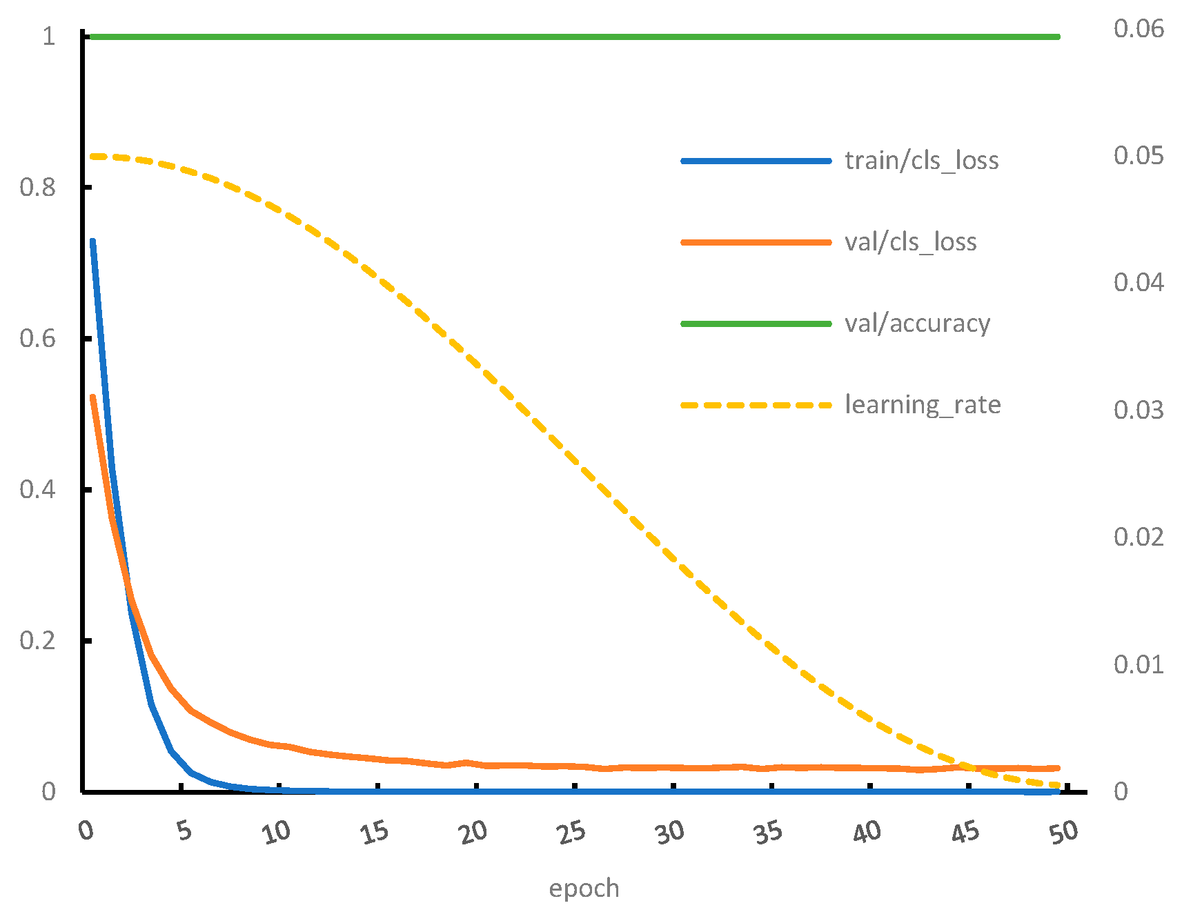
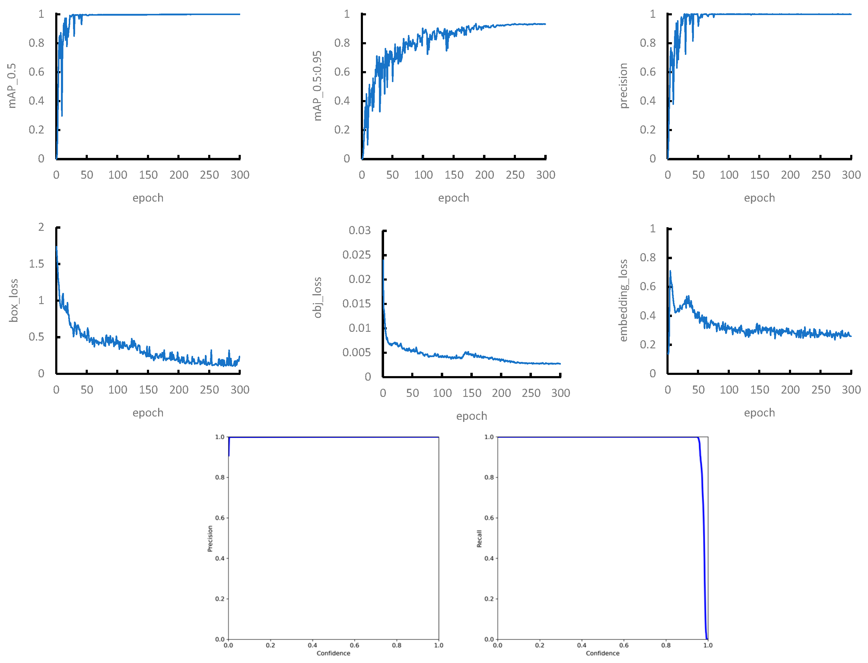
3.2.4. The Convergence of the Model

To demonstrate the convergence of the model on the given dataset, Figure 13 illustrates the evolution of loss components and performance metrics throughout the training process of the YOLOv7 model. The x-axis denotes the iteration count, while the y-axis measures the values of loss and metrics. The graph indicates that the model achieves stable performance, with minimal fluctuations in loss and metric values, after undergoing 300 iterations. One thing worth noting is the behavior of the embedding loss, which initially experiences a sharp increase followed by a gradual decrease. This pattern suggests that in the early stages of training, the model struggles to accurately identify targets, leading to calculations involving few to no values. This phenomenon similarly impacts the mAP; as the model begins to recognize some targets, the subsequent rise in embedding loss influences the weight adjustments, temporarily causing fluctuations in the mAP before it stabilizes. Furthermore, the curve of precision and recall versus confidence indicates that the model is capable of accurately identifying fans in the scene.

3.3. Object Tracking and Region Extraction

To assess the efficacy of region extraction in mitigating computational demands, we executed a series of experiments on an edge computing framework. These experiments were designed to facilitate a comparative analysis by performing inference on identical segments of video surveillance footage, thereby evaluating the inference latency across varying window dimensions. Our edge computing platform is RK3399Pro, which integrates an NPU dedicated to neural network computing. Our investigation delineates the computational process into two primary segments: neural network inference conducted by the NPU and post-processing. Furthermore, we conducted evaluations to ascertain the impact of varying pruning rates on model performance using DepGraph [23].

Table 1. Detection time consumption under different window sizes.

Pruning Ratio	Window Size	Average Inference Time	Average Post-Processing Time	Number of Target Losses
0%	-	327.43	4.54	0
	128	162.76	8.50	18
	96	135.22	5.94	17
	64	111.32	3.58	20
50%	-	247.35	4.90	0
	128	128.77	7.18	9
	96	104.66	5.36	6
	64	83.06	3.02	7
62.5%	-	242.01	4.87	6
	128	118.63	6.70	4
	96	107.70	5.62	34
	64	80.66	2.83	7
75%	-	220.15	4.70	0
	128	122.24	5.50	28
	96	93.36	3.36	15
	64	58.20	0.91	48

Full frame detection is used every 16 frames.

demonstrates that the utilization of ROI extraction techniques can effectively reduce the inference time of the model. A reduction in the detection window size leads to decreased inference time. Furthermore, there is an increase in post-processing time when using a detection window, which can be attributed to the need to manage a larger number of duplicate targets with high confidence levels, particularly when these targets are nearby. Additionally, a reduction in the size of the detection window is associated with a decrease in detection accuracy, which in turn results in the loss of targets.

4. Conclusions

This study introduces a novel method for detecting the state of equipment, specifically pan-tilt cameras used within greenhouses, thereby maximizing the potential of an existing camera. It offers two significant enhancements to reduce computational load: Firstly, it integrates object detection with embedding to eliminate redundant feature extraction in both detection and state recognition phases. By augmenting YOLOv7’s output and jointly training it with a decoding network, we enable simultaneous object detection and embedding. Our experiments demonstrate that the embeddings generated capture the semantic details of the object’s state, allowing the operational condition of greenhouse fans to be accurately inferred through straightforward machine-learning techniques. Secondly, we optimize computational resources by focusing on predicted areas of interest, thereby minimizing the analysis of non-relevant zones. Our findings on RK3399Pro, an edge computing platform, reveal that this approach achieves a significant reduction in inference time, exceeding 50%, with minimal impact on accuracy.

References

1. Zhou, L.; Song, L.; Xie, C.; Zhang, J. Applications of Internet of Things in the Facility Agriculture. In Proceedings of the Computer and Computing Technologies in Agriculture VI, Zhangjiajie, China, 19–21 October 2012; Li, D., Chen, Y., Eds.; Springer: Berlin/Heidelberg, Germany, 2013; pp. 297–303. [Google Scholar]
2. Chaux, J.D.; Sanchez-Londono, D.; Barbieri, G. A Digital Twin Architecture to Optimize Productivity within Controlled Environment Agriculture. Appl. Sci. 2021, 11, 8875. [Google Scholar] [CrossRef]
3. Li, H.; Guo, Y.; Zhao, H.; Wang, Y.; Chow, D. Towards automated greenhouse: A state of the art review on greenhouse monitoring methods and technologies based on internet of things. Comput. Electron. Agric. 2021, 191, 106558. [Google Scholar] [CrossRef]
4. Hassan, I.U.; Panduru, K.; Walsh, J. An In-Depth Study of Vibration Sensors for Condition Monitoring. Sensors 2024, 24, 740. [Google Scholar] [CrossRef] [PubMed]
5. Qin, L.; Huang, Y.; Yunmeng, G.; Shi, C. Design and Experiment of Status Detection of Greenhouse Ventilation Devices. Trans. Chin. Soc. Agric. Mach. 2021, 52, 303–311. [Google Scholar]
6. Liu, W.; Kang, G.; Huang, P.-Y.; Chang, X.; Yu, L.; Qian, Y.; Liang, J.; Gui, L.; Wen, J.; Chen, P. Argus: Efficient Activity Detection System for Extended Video Analysis. In Proceedings of the 2020 IEEE Winter Conference on Applications of Computer Vision Workshops (WACVW), Snowmass, CO, USA, 1–5 March 2020; IEEE: New York, NY, USA, 2020; pp. 126–133. [Google Scholar]
7. Lao, W.; Cui, C.; Zhang, D.; Zhang, Q.; Bao, Y. Computer Vision-Based Autonomous Method for Quantitative Detection of Loose Bolts in Bolted Connections of Steel Structures. Struct. Control Health Monit. 2023, 2023, 8817058. [Google Scholar] [CrossRef]
8. Ting, L.; Khan, M.; Sharma, A.; Ansari, M.D. A secure framework for IoT-based smart climate agriculture system: Toward blockchain and edge computing. J. Intell. Syst. 2022, 31, 221–236. [Google Scholar] [CrossRef]
9. Sengupta, A.; Gill, S.S.; Das, A.; De, D. Mobile Edge Computing Based Internet of Agricultural Things: A Systematic Review and Future Directions. In Mobile Edge Computing; Mukherjee, A., De, D., Ghosh, S.K., Buyya, R., Eds.; Springer International Publishing: Cham, Switzerland, 2021; pp. 415–441. ISBN 978-3-030-69893-5. [Google Scholar]
10. Zheng, X.; Chen, F.; Lou, L.; Cheng, P.; Huang, Y. Real-Time Detection of Full-Scale Forest Fire Smoke Based on Deep Convolution Neural Network. Remote Sens. 2022, 14, 536. [Google Scholar] [CrossRef]
11. Sun, P.; Jiang, Y.; Xie, E.; Shao, W.; Yuan, Z.; Wang, C.; Luo, P. What Makes for End-to-End Object Detection? arXiv 2021, arXiv:2012.05780. [Google Scholar] [CrossRef]
12. Lai, T. Real-Time Aerial Detection and Reasoning on Embedded-UAVs in Rural Environments. IEEE Trans. Geosci. Remote Sens. 2023, 61, 4403407. [Google Scholar] [CrossRef]
13. Zheng, X.; Lu, C.; Zhu, P.; Yang, G. Visual Multitask Real-Time Model in an Automatic Driving Scene. Electronics. 2023, 12, 2097. [Google Scholar] [CrossRef]
14. Wang, C.-Y.; Bochkovskiy, A.; Liao, H.-Y.M. YOLOv7: Trainable bag-of-freebies sets new state-of-the-art for real-time object detectors. arXiv 2022, arXiv:2207.02696. [Google Scholar] [CrossRef]
15. Chen, S.; Guo, W. Auto-Encoders in Deep Learning—A Review with New Perspectives. Mathematics 2023, 11, 1777. [Google Scholar] [CrossRef]
16. Zheng, Z.; Wang, P.; Liu, W.; Li, J.; Ye, R.; Ren, D. Distance-IoU Loss: Faster and Better Learning for Bounding Box Regression. arXiv 2019, arXiv:1911.08287. [Google Scholar] [CrossRef]
17. Yang, Y.; Zhou, Y.; Yue, X.; Zhang, G.; Wen, X.; Ma, B.; Xu, L.; Chen, L. Real-time detection of crop rows in maize fields based on autonomous extraction of ROI. Expert Syst. Appl. 2023, 213, 118826. [Google Scholar] [CrossRef]
18. Han, C.; Zheng, K.; Zhao, X.; Zheng, S.; Fu, H.; Zhai, C. Design and Experiment of Row Identification and Row-oriented Spray Control System for Field Cabbage Crops. Trans. Chin. Soc. Agric. Mach. 2022, 53, 89–101. [Google Scholar]
19. Ghahremannezhad, H.; Shi, H.; Liu, C. A New Adaptive Bidirectional Region-of-Interest Detection Method for Intelligent Traffic Video Analysis. In Proceedings of the 2020 IEEE Third International Conference on Artificial Intelligence and Knowledge Engineering (AIKE), Laguna Hills, CA, USA, 9–13 December 2020; pp. 17–24. [Google Scholar]
20. Bewley, A.; Ge, Z.; Ott, L.; Ramos, F.; Upcroft, B. Simple online and realtime tracking. In Proceedings of the 2016 IEEE International Conference on Image Processing (ICIP), Phoenix, AZ, USA, 25–28 September 2016; pp. 3464–3468. [Google Scholar]
21. Wang, Z.; Bovik, A.C.; Sheikh, H.R.; Simoncelli, E.P. Image quality assessment: From error visibility to structural similarity. IEEE Trans. Image Process. 2004, 13, 600–612. [Google Scholar] [CrossRef] [PubMed]
22. Hotelling, H. Analysis of a complex of statistical variables into principal components. J. Educ. Psychol. 1933, 24, 417–441. [Google Scholar] [CrossRef]
23. Fang, G.; Ma, X.; Song, M.; Mi, M.B.; Wang, X. DepGraph: Towards Any Structural Pruning. In Proceedings of the IEEE/CVF Conference on Computer Vision and Pattern Recognition (CVPR), Vancouver, BC, Canada, 17–24 June 2023; pp. 16091–16101. [Google Scholar]
Figure 1. The reduction of feature maps across YOLOv7. The dashed boxes in the figures signify changes introduced in our study, elaborated in subsequent sections.
Applsci 14 03378 g001
Figure 2. An autoencoder.
Applsci 14 03378 g002
Figure 3. A comparative analysis of inference methodologies: traditional vs. integrated detection–embedding frameworks.
Applsci 14 03378 g003
Figure 4. Model Training Schematic.
Applsci 14 03378 g004
Figure 5. Fan monitoring in a greenhouse environment.
Applsci 14 03378 g005
Figure 6. Methodological data flow diagram.
Applsci 14 03378 g006
Figure 7. (a) CIOU schematic diagram; (b) comparison of IoU and CIOU in different overlapping situations.
Applsci 14 03378 g007
Figure 8. Experimental setup.
Applsci 14 03378 g008
Figure 9. SSIM change curve under different reconstruction loss functions and scaling strategies during the training phase.
Applsci 14 03378 g009
Figure 10. Impact of enhancement techniques on image reconstruction. The colored image is the original image, and the grayscale image is the reconstructed image. (a) Normalization; (b) gamma transformation; (c) histogram equalization.
Applsci 14 03378 g010
Figure 11. The distribution of embedding after PCA. Each colored dot represents an embedding. The dots in the red circles represent the stopped fans.
Applsci 14 03378 g011
Figure 12. Changes in various metrics during model training (where the learning rate corresponds to the right y-axis and the rest correspond to the left y-axis).
Applsci 14 03378 g012
Figure 13. Loss components and performance metrics.
Applsci 14 03378 g013