Abstract
As the leading platform of online education, MOOCs provide learners with rich course resources, but course designers are still faced with the challenge of how to accurately improve the quality of courses. Current research mainly focuses on learners’ emotional feedback on different course attributes, neglecting non-emotional content as well as the costs required to improve these attributes. This limitation makes it difficult for course designers to fully grasp the real needs of learners and to accurately locate the key issues in the course. To overcome the above challenges, this study proposes an MOOC improvement method based on text mining and multi-attribute decision-making. Firstly, we utilize word vectors and clustering techniques to extract course attributes that learners focus on from their comments. Secondly, with the help of some deep learning methods based on BERT, we conduct a sentiment analysis on these comments to reveal learners’ emotional tendencies and non-emotional content towards course attributes. Finally, we adopt the multi-attribute decision-making method TOPSIS to comprehensively consider the emotional score, attention, non-emotional content, and improvement costs of the attributes, providing course designers with a priority ranking for attribute improvement. We applied this method to two typical MOOC programming courses—C language and Java language. The experimental findings demonstrate that our approach effectively identifies course attributes from reviews, assesses learners’ satisfaction, attention, and cost of improvement, and ultimately generates a prioritized list of course attributes for improvement. This study provides a new approach for improving the quality of online courses and contributes to the sustainable development of online course quality.
1. Introduction
Massive Open Online Courses (MOOCs), a significant innovation in teaching technology, offer a diverse array of high-quality open online courses globally [1], effectively overcoming numerous limitations of traditional offline learning in terms of cost, space, and background [2,3]. Simultaneously, the openness of MOOCs presents a novel opportunity for higher education institutions to create a richer and enhanced learning experience for learners through strengthened collaboration in knowledge sharing [4]. The emergence of MOOCs has not only facilitated the global sharing of educational resources but has also breathed new life into educational equity and popularization efforts [5]. MOOCs are now at the forefront of education [6]. Since the inception of the “Year of MOOCs” in 2012, the utilization of MOOCs has been steadily increasing worldwide. This trend has been further accelerated by the COVID-19 pandemic, which prompted the transition of numerous offline courses to online formats [7]. Consequently, people have become increasingly reliant on MOOCs, with millions of new users signing up on their platforms [8]. By 26 January 2024, China had launched over 76,800 MOOCs, catering to a staggering 1.277 billion learners within the country. MOOCs are now at the forefront of education [9].
However, despite the booming development of MOOCs, the rapid surge in the number of courses has given rise to numerous challenges, including a high dropout rate [10,11,12] and inconsistent quality [13], thereby hampering the sustainable progress of MOOCs. Since learner satisfaction plays a pivotal role in extending the duration of product usage [14], it has become imperative to pinpoint the issues prevailing in MOOCs and furnish targeted recommendations to course designers, aiming to enhance learner satisfaction.
MOOCs enable learners to share their views and perceptions of courses through posted reviews. These reviews encompass a diverse array of learner needs, expectations, and suggestions [15], serving as a rich resource for enhancing course quality. By delving deeply into these comments, we can gain insights into the learners’ satisfaction and dissatisfaction levels towards various course attributes [16], enabling us to provide targeted improvement directions to course designers [17], such as the research of Geng et al. [18] and Liu et al. [19].
Text mining is the process of extracting valuable information from text data [20]. By analyzing the satisfaction and dissatisfaction expressed by reviewers, valuable insights can be gained into consumer requirements, which in turn can guide product improvements [21,22,23]. For the product attributes that people are less satisfied with, it may be the product attributes that need to be improved [24,25]. These studies usually first mine the attributes of the product or service from the reviews, as well as the sentiment related to the attribute, and then determine the satisfaction and attention to the attribute. Ultimately, the decision on which attributes require improvement is made based on a combination of satisfaction levels and attention received from customers.
Text mining can also be employed to identify attributes in MOOCs that learners are dissatisfied with, enabling instructors to subsequently target these attributes for improvement.
However, there is a relative lack of research on MOOC improvement through text mining, and previous studies rarely considered the non-emotional content and improvement cost of product attributes. Indeed, online reviews encompass both emotional and non-emotional content, both of which are equally valuable for analysis [26]. One of the primary reasons that individuals write online reviews on e-commerce platforms is to alleviate consumer uncertainty during the shopping process [27]. Therefore, we can infer that the non-emotional reviews penned by learners on MOOCs serve to assist those reading the reviews in better comprehending the course content. Therefore, we can infer that the non-emotional reviews written by learners on MOOCs are meant to help the readers of the reviews understand the course content better. In turn, the attributes contained in non-emotional reviews may be important to future learners, in a reviewer’s opinion.
When determining which product attributes require improvement, the associated cost is a critical consideration. In the realm of product development, cost often serves as a pivotal factor in prioritizing attribute enhancements [28]. Similarly, the same principle applies to course improvement. If learners express dissatisfaction with a particular course attribute but the cost of enhancing that attribute is substantial, it may not necessarily receive a high priority for improvement. Alternatively, even if learners express satisfaction with a particular attribute, it may still be prioritized for improvement if the cost of enhancing it is relatively low.
Hence, a comprehensive approach is necessary for course improvement, considering learner satisfaction, non-emotional content, attention, and the cost of enhancing various attributes. This makes it a multi-attribute decision-making (MADM) problem to identify course attributes that need to be improved. MADM refers to the problem of making decisions for multiple alternatives with multiple evaluation criteria [29].
To address the aforementioned problems, we aim to introduce a novel approach that integrates text mining and multi-attribute decision-making (MADM) for the improvement of MOOCs. This framework will enable us to extract course attributes that learners prioritize, along with their emotional and non-emotional responses towards these attributes. Subsequently, it will provide recommendations for course enhancement.
2. Related Work
In this section, we review works that are pertinent to our topic. Specifically, we consider recent studies focusing on MOOC review text mining, as well as those that explore product or service improvement through review text mining.
2.1. MOOC Review Text Mining
As the accumulation of learner reviews continues to grow on MOOC platforms and text mining technology becomes more sophisticated, there has been a surge in research exploring the analysis of MOOC review texts.
Kastrati et al. [30] proposed a weakly supervised aspect-based sentiment analysis method for MOOC reviews, which can effectively reduce the dependence of the model on the number of training samples. Mrhar et al. [31] proposed a sentiment analysis method that combines Bayesian neural networks, convolutional neural networks (CNNs), and long short-term memory (LSTM). This method demonstrates promising results in the sentiment analysis of MOOC comments. Wang et al. [32] employed the ALBERT-BiLSTM model for sentiment analysis of MOOC reviews, revealing superior performance compared to existing methodologies. To enable data-driven design automation, Dina et al. [33] proposed a text-mining-based approach that automatically extracts feature sentiment pairs from MOOC reviews. In order to improve the performance of sentiment analysis, Liu et al. [34] combined BERT and part-of-speech information in MOOC reviews of sentiment. Liu et al. [35] proposed an MOOC-BERT model to automatically identify learners’ cognition from online reviews, which has been verified to be superior to representative deep learning models in recognition and cross-curriculum.
Lundqvist et al. [36] categorized learners in MOOCs into beginner, experienced, and unknown categories and conducted a comparative analysis of the attitude differences among these learner groups in MOOCs. To gain insights into learners’ preferences and concerns, Geng et al. [18] employed a combination of machine learning techniques and statistical analyses to mine reviews from NetEase, and they found learners pay more attention to the teaching and platform rather than the course content. Hew et al. [37] identified the influencing factors of learner satisfaction through text mining techniques. Nie et al. [38] introduced a comprehensive scoring methodology for MOOCs. This approach initially mined individuals’ satisfaction levels with various course aspects from MOOC reviews, subsequently employing the Analytic Hierarchy Process (AHP) to generate an overall course rating. Chen et al. [39] used a structural topic model in MOOC reviews and found that the topics vary depending on the emotions or categories of the courses involved. Li et al. [6] undertook a comprehensive investigation to identify the key factors that contribute to the success of MOOCs. They categorized MOOCs into two distinct types and conducted a detailed analysis to uncover the influencing factors associated with each type. Gomez et al. [9] performed an extensive analysis of a large corpus of review text data, uncovering that numeric ratings alone provide limited guidance to learners in the course selection process. However, they identified that text mining can be effectively employed to aid course selection, as MOOC reviews contain abundant valuable information. Nilashi et al. [40] introduced a multi-stage text-mining-driven approach aimed at uncovering the influencing factors of learner satisfaction in MOOCs. Furthermore, to ensure the reliability and practical implications of their proposed method, they validated its efficacy through a survey methodology. Based on online reviews, Wang et al. [41] discovered that not all online review topics exert an influence on overall learner satisfaction.
It is evident that recent research on MOOC text mining has primarily focused on methodological studies, with a strong emphasis on extracting valuable content from MOOC reviews. Notably, there has been a significant focus on exploring the influencing factors of learner satisfaction. However, a notable gap exists in the literature regarding the provision of course improvement suggestions based on these mined influencing factors. This study aims to bridge this gap and provide practical recommendations for enhancing the quality of MOOCs and learner satisfaction.
2.2. Review Text-Mining-Based Product or Service Improvement
Online reviews encompass consumers’ varying degrees of satisfaction and dissatisfaction towards various products or services. Consequently, numerous studies have been devoted to the text mining of online reviews, aiming to facilitate product enhancement and the creation of innovative offerings.
Zhou et al. [24] utilized Latent Dirichlet Allocation (LDA) [42] to extract product attributes from Amazon reviews. Subsequently, they employed a rule-based sentiment analysis approach to categorize the sentiment associated with these attributes. Finally, they leveraged the Kano model to identify the attributes that required improvement. Their approach is a typical approach of text-mining-based product improvement, such as Lee et al. [25]. Liu et al. [43] enhanced the efficacy of the traditional Kano model for product improvement by integrating it with the fuzzy Analytic Hierarchy Process (AHP) and Quality Function Deployment (QFD). This integrated approach provided a comprehensive framework for prioritizing and optimizing product attributes, leading to more targeted and effective product enhancements. Chen et al. [44] undertook a comprehensive text mining analysis of high-speed rail reviews, successfully extracting six passenger demands. Utilizing large-scale group decision-making techniques, they aggregated the satisfaction levels of 100 passengers across these six demands, finally deriving the six demands’ degrees of satisfaction and rankings. Chen et al. [22] took into account both explicit and implicit features during the extraction of product attributes. They employed neural network training to determine the relative importance of each feature, subsequently mapping these attributes to the Kano model. Previous studies employing text mining and the Kano model have not considered the consumers’ affective needs. In order to address this issue, Jin et al. [45] adopted the Kansei-integrated Kano method to obtain the priority of product feature improvement. This method incorporates affective design and is more comprehensive than the traditional Kano model. Goldberg et al. [46] used the attribute mapping framework introduced by MacMillan and McGrath, successfully extracting attributes from reviews to offer innovation insights. Their approach to mining attributes from online reviews surpasses previous methods in terms of depth and precision. Huang et al. [47] combined the Latent Dirichlet Allocation (LDA) topic model and Quality Function Deployment (QFD) to mine customer requirements and competition information from online reviews for new product development. Ji et al. [48] proposed a large-scale group decision-making method to integrate the satisfaction of individual consumers on product attributes to form group satisfaction. Joung and Kim [49] utilized text mining techniques to cluster consumers based on their preferences. Initially, they mined the product attributes that consumers prioritize from online reviews. Subsequently, they employed neural networks to determine the importance of these attributes and clustered consumers accordingly, leveraging the attribute importance weights. Zhang and Song [50] combined text mining and large group decision-making methods to make product improvement decisions. Through a comparative analysis with intuitive and expert decision-making approaches, they demonstrated the reliability and effectiveness of their proposed method, surpassing both comparison methods. While numerous studies have primarily centered on enhancing products or services through text mining, often neglecting non-emotional content and the associated costs of attribute improvement, they primarily focus on consumer attention and satisfaction.
2.3. Review the Ranking Method of Multi-Attribute Decision-Making
Whether it be a purchase decision in daily life or a task scheduling decision at work, decision-making forms a crucial aspect of people’s daily lives and professional endeavors [51]. Some decisions can be relatively straightforward, with minor consequences if a wrong choice is made. However, other decisions can be highly intricate, such that even a slight error can lead to significant repercussions, necessitating a profound and cautious approach. Generally speaking, a decision problem in real life typically involves numerous criteria or attributes that must be taken into account concurrently to arrive at a well-informed decision. The exploration of such challenges is frequently labeled as multi-criterion decision-making or multi-attribute decision-making, which entails selecting the most suitable option from a finite set of alternatives.
The literature introduces some of the most renowned MADM methods, including PROMETHEE, TODIM, VIKOR, and TOPSIS, which are designed to tackle ranking problems effectively [52,53,54,55]. Qin et al. [56] initially extracted product attributes, weight values, and emotional tendencies from online reviews. Subsequently, they employed the Random Multi-criteria Acceptance Analysis (SMAA)-PROMETHEE method, to derive product ranking outcomes. Zhang et al. [57] proposed an innovative product selection model that integrates sentiment analysis with the intuitionistic fuzzy TODIM method. This model aims to assist potential customers in ranking alternative products based on consumers’ opinions regarding product performance. Liang et al. [51] introduced a quantitative approach for hotel selection leveraging online reviews. Furthermore, they innovatively developed the DL-VIKOR method, which ranks hotels based on customer satisfaction scores and the weights of extracted attributes. Nilashi et al. [58] conducted a cluster analysis using self-organizing mapping (SOM) to categorize hotel features. Subsequently, they employed the similarity to Ideal Solution Prioritization technique (TOPSIS) to rank these features. Additionally, neural fuzzy technology was utilized to reveal customer satisfaction levels, providing a comprehensive understanding of hotel performance. Li et al. [55] introduced a novel approach for product ranking that integrates the mining of online reviews with an interval-valued intuitionistic fuzzy technique (TOPSIS). This method aims to assist consumers in selecting products that align with their individual preferences.
No single multi-attribute decision analysis method (MADM) can be unilaterally designated as the best or worst, as each has its own unique strengths and limitations [59]. Each MADM method possesses distinct advantages and limitations, and its effectiveness depends heavily on how it is tailored to specific outcomes and objectives within the planning process. Consequently, the selection of an appropriate MADM model should be guided by specific scenarios and requirements rather than solely relying on general evaluations. TOPSIS, originally developed by Hwang and Yoon in 1981, is a straightforward ranking method, both conceptually and in terms of its application [60]. TOPSIS offers three notable benefits: it is comprehensive; it requires minimal data; and it produces intuitive and easily comprehensible results [55]. Given its excellent performance in our investigation [61], the method combining the interval intuitionistic fuzzy set with TOPSIS was chosen as the ranking method for this study.
After considering the above studies, we first use text mining techniques to extract the attributes that learners pay attention to, the corresponding emotional tendency and attention degree of the attributes from online reviews, and determine the satisfaction degree of the attributes. We then use a multi-attribute decision-making approach to prioritize attribute improvements.
3. Methods
Our objective is to leverage text mining techniques in MOOC reviews to identify priority areas for improvement in MOOC attributes. Our method consists of the following steps: (1) collection and preprocessing of data; (2) extraction of course attributes; (3) identification of emotional and non-emotional content linked to the course attributes; (4) ascertainment of the cost associated with attribute improvements; and (5) generation of a prioritized list of attribute improvements (see Figure 1).

Figure 1.
Overall steps of our method.
3.1. Data Collection and Preprocessing
We implemented a Python crawler to scrape online reviews on MOOC platforms. After that, we conducted the following preprocessing:
Step 1: Removing duplicate reviews. Removing duplicate reviews can help us improve the efficiency and quality of text mining.
Step 2: Text segmentation. As some reviews are long in length, they may contain multiple course keywords. We first used symbols (e.g., “.”, “?”, “!”, “…”) to segment longer reviews into short sentences, trying to make each sentence contain only one course keyword. Then we segmented the sentences into word lists to facilitate course attribute extraction and sentiment analysis.
Step 3: Removing stop words, including meaningless punctuation (e.g., !?#@). Removing stop words not only prevents subsequent steps from wasting time on non-informative words but also enhances the accuracy and efficiency of determining emotional and non-emotional content. As we intend to employ deep-learning-based text classification methods for the identification of emotional and non-emotional content, the presence of stop words can potentially compromise the performance of these models.
Step 4: Data labeling. Given that our sentiment analysis task relies on machine learning algorithms, labeled datasets are essential for training classifiers. Therefore, it is imperative to label the data, classifying them into four distinct categories: positive, negative, neutral, and non-emotional.
Step 5: Part-of-speech tagging. To extract alternative attribute words for courses, which are typically nouns, we must first determine the part-of-speech of each word in the course reviews.
Among them, for word segmentation and part-of-speech tagging, we utilized the jieba word segmentation tool, a highly renowned Chinese word segmentation utility in Python.
3.2. Course Attributes Extraction
Previous studies mainly used the LDA topic model or word embedding to extract and classify product attributes, where word embedding methods do not require manual interpretation of each topic [49]. Therefore, we used the word embedding method to extract and classify course attributes. Our approach consisted of the following steps:
Step 1: Nouns were extracted from all the reviews for a course, that is, words that start with “n” in the POS tags. Course attributes are usually nouns, so we extract the nouns in course reviews as our alternative attribute words. The number of extracted nouns is usually large, and the main attributes of a course may be limited to a few, so we needed to find a way to cluster these nouns and then treat each cluster as an attribute. Clustering algorithms usually take input in vector form, so we needed to convert nouns into vector form.
Step 2: To convert the selected nouns into a vectorized format, we employed the FastText word embedding approach. Word embedding is a technique that maps words onto a vector space, allowing each word to be represented by a unique vector. Furthermore, words with similar meanings tend to have word vectors that are proximate in Euclidean space. This characteristic makes word embedding an ideal approach for converting words into vectors and subsequently clustering them. A representative word embedding method is FastText [62], which considers the morphology of words, that is, the n-grams of word characters. For example, the 2-g of the word “where” includes “wh”, “he”, “er”, and “re”. FastText for words that do not occur during training can be represented by the sum of its character n-grams, which allows FastText to represent any word. The pre-trained Chinese FastText word vectors (https://dl.fbaipublicfiles.com/fasttext/vectors-crawl/cc.zh.300.bin.gz (accessed on 1 February 2024)) are used to represent the nouns in our work.
Step 3: For noun clustering, we employed a combined approach incorporating Affinity Propagation (AP) clustering [63] and manual intervention. AP is one of the most classical and widely used clustering methods that clusters the close words into the same cluster and the far words into different clusters by calculating the distance. A significant advantage of AP clustering is that it does not require the specification of the number of clusters upfront. After AP clustering, we manually proofread the clustering results to make the meaning of words in each cluster as close as possible and delete meaningless words.
Step 4: The words in each cluster after clustering are induced to summarize the course attributes. By summarizing the nouns in each cluster into attributes, we can know the main attributes of a course that learners pay attention to.
Step 5: The nouns’ frequency of different attributes was counted, as was the total word frequency of an attribute. This approach is based on the assumption that a higher frequency of an attribute word indicates greater learner attention and importance placed on that specific attribute.
3.3. Determination of the Emotional and Non-Emotional Content Corresponding to the Course Attributes
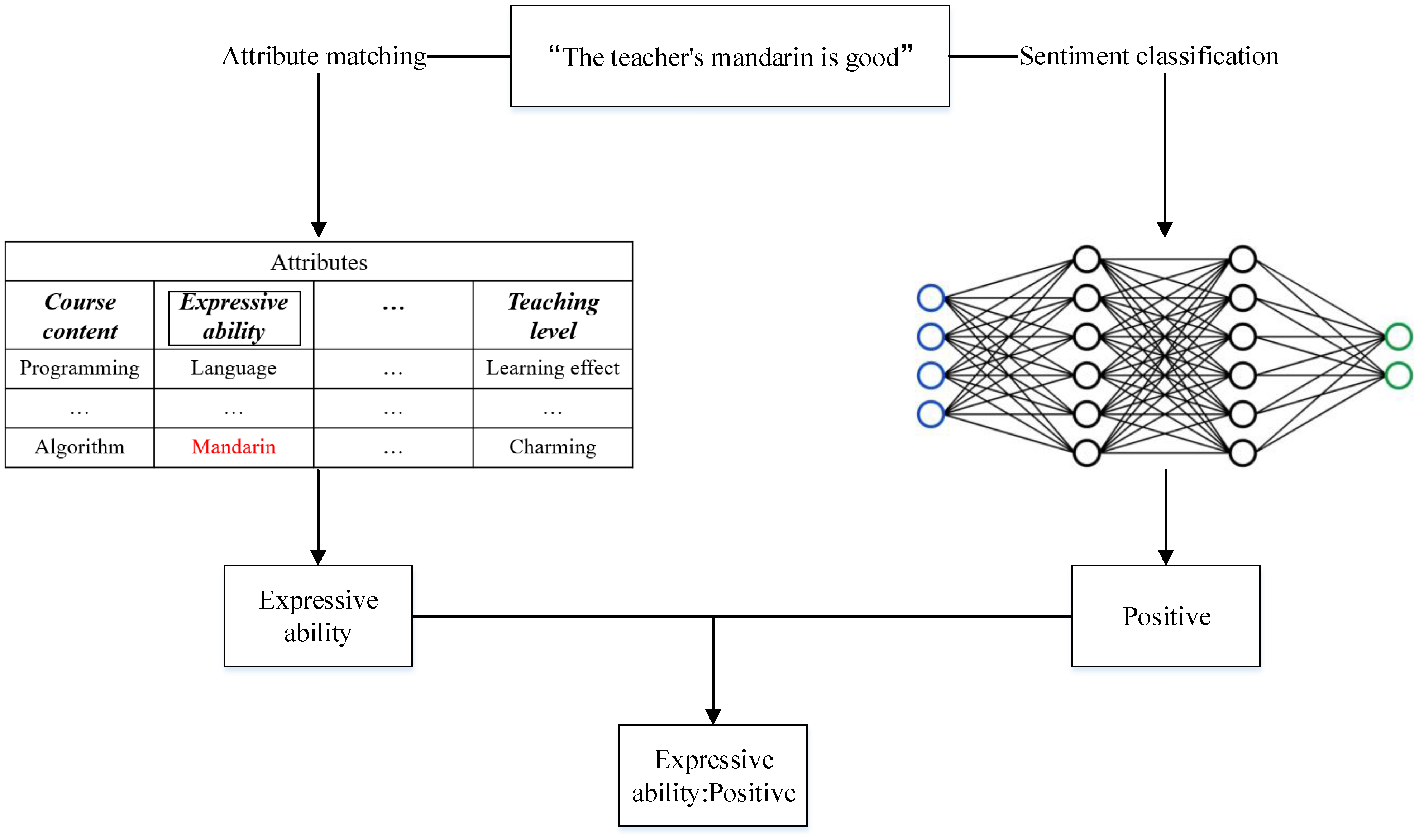
To identify the emotional and non-emotional content associated with the course attributes, we built a deep-learning-based text classification model. This model was trained to categorize review text into four distinct classes: positive, negative, neutral, and non-emotional. For ease of presentation, the classification of a review belonging to these four classes was collectively referred to as sentiment classification. We used a simple means to determine the course attribute and its corresponding sentiment class in a review: if a review contains a word belonging to an attribute whose sentiment tendency has been determined to be non-emotional, we consider the attribute to be non-emotional in this review. For example, in the sentence “The teacher’s mandarin is good”, obviously, this is a positive review, and if mandarin belongs to the attribute “expressive ability”, we can assume that the emotional tendency of expressive ability in this sentence is positive (see Figure 2). We have highlighted the keywords that appear in the sentence in red in the Figure 2 and highlighted the corresponding attribute in the box. First and foremost, we carefully selected a specific number of comments from the vast pool of online feedback to be manually annotated. Positive sentiment comments are labeled as 1, negative sentiment as −1, neutral sentiment as 0, and comments lacking emotional expression are designated as 2. Subsequently, a subset of these annotated comments was utilized to train a deep learning model, while the remaining comments served as a validation set to assess the model’s accuracy. After rigorous testing, the model exhibiting the highest predictive accuracy was chosen to analyze the emotional tendencies of the remaining unlabeled comments.
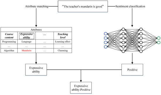
Figure 2.
The way to determine the course attribute and its corresponding sentiment class in a review.
The pivotal aspect lies in developing a deep-learning-based sentiment classification model that can effectively categorize and analyze the sentiment expressed in reviews. The reason why we choose deep learning for sentiment classification is that in recent years, deep learning has gradually become the mainstream model for sentiment classification, and with the help of pre-trained language models such as BERT [64], the accuracy of sentiment classification has also been greatly improved. Deep learning is a machine learning technique rooted in artificial neural networks, requiring the integration of various deep learning modules to construct a complete model. Our deep-learning-based sentiment classification model is structured into three distinct modules: the embedding layer, the intermediate layer, and the output layer.
3.3.1. Embedding Layer
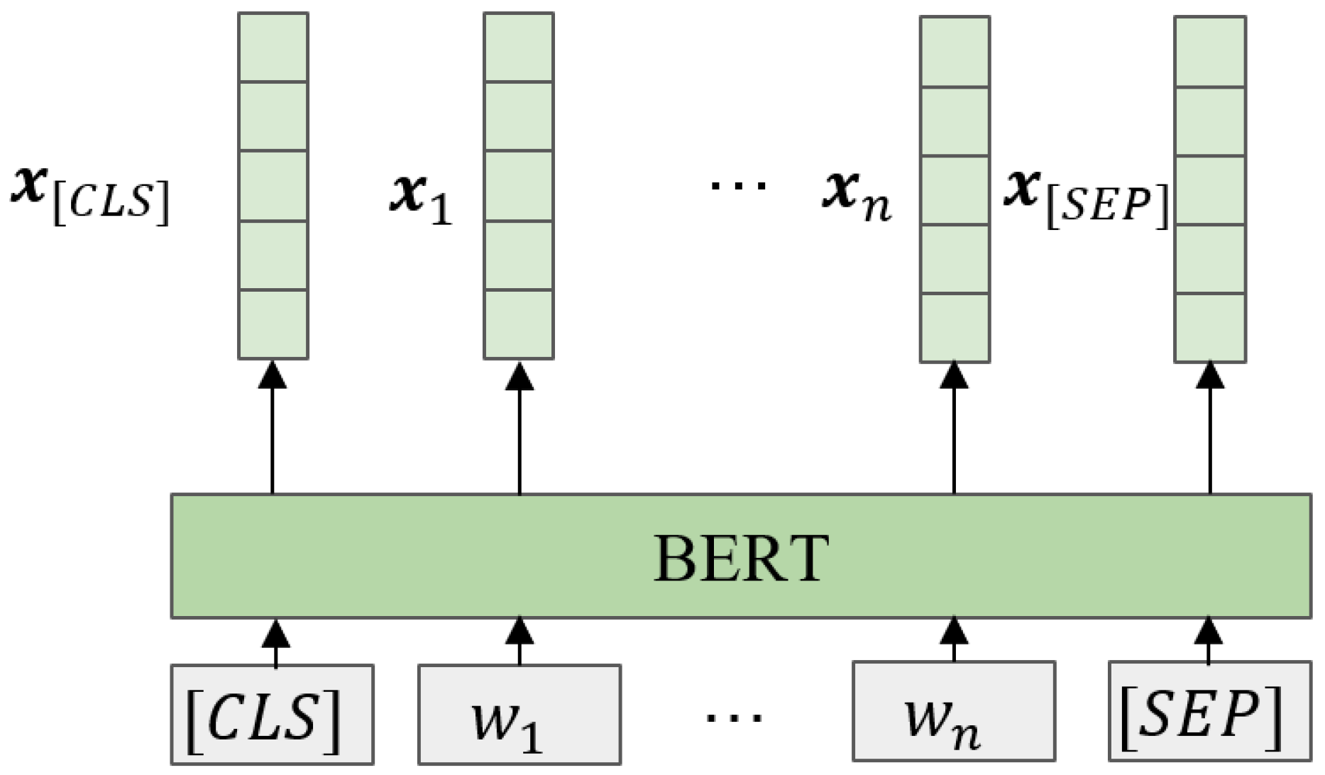
As previously mentioned in Section 3.2, word embeddings serve as a mechanism to transform words into a vectorized format. The embedding layer specifically handles the vectorization of words within the deep learning model. We utilized the BERT model directly for word embedding due to its exceptional performance in downstream tasks, particularly sentiment classification. In this paper, we directly used Chinese BERT (https://huggingface.co/bert-base-chinese (accessed on 2 February 2024)) pre-trained by Hugging Face to help us with word embedding. Hugging Face (https://huggingface.co/ (accessed on 1 February 2024)) is an artificial intelligence community, providing people with a large number of artificial intelligence code and application programming interface (API), so that people can implement artificial intelligence with low cost. The inputs and outputs in BERT-based embedding can be seen in Figure 3.
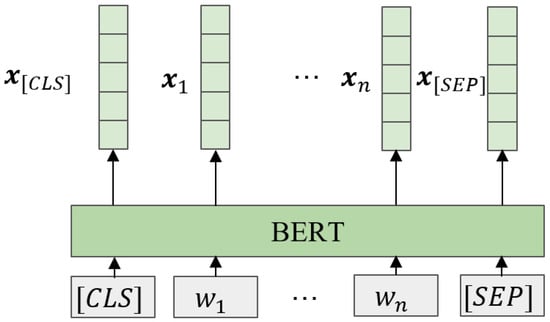
Figure 3.
The input and output of BERT-based embedding.
The inputs in BERT embedding are words (for English) or characters (for Chinese) of a sentence, which are [CLS], , , …, , [SEP], where , , …, are words or characters of a sentence of length n (the number of English words or Chinese characters), “[CLS]” is a symbol specifically used for text classification, and “[SEP]” represents a sentence separator or terminator. When we input sentences, Hugging Face automatically adds these two symbols to the original sentences without us having to manually do so. The outputs are , , …, , and , which are the vector representation of all inputs.
3.3.2. Intermediate Layer
Compared with the embedding layer and output layer, which are relatively fixed, the intermediate layer changes more. In order to avoid using only one intermediate layer and resulting in poor performance of the trained classifier, we compared six intermediate layers: base BERT, feed-forward neural network (FFNN), CNN, LSTM, LSTM combined with attention mechanism (LSTM + attention), and LSTM combined with CNN (LSTM + CNN).
- (1)
- Base BERT
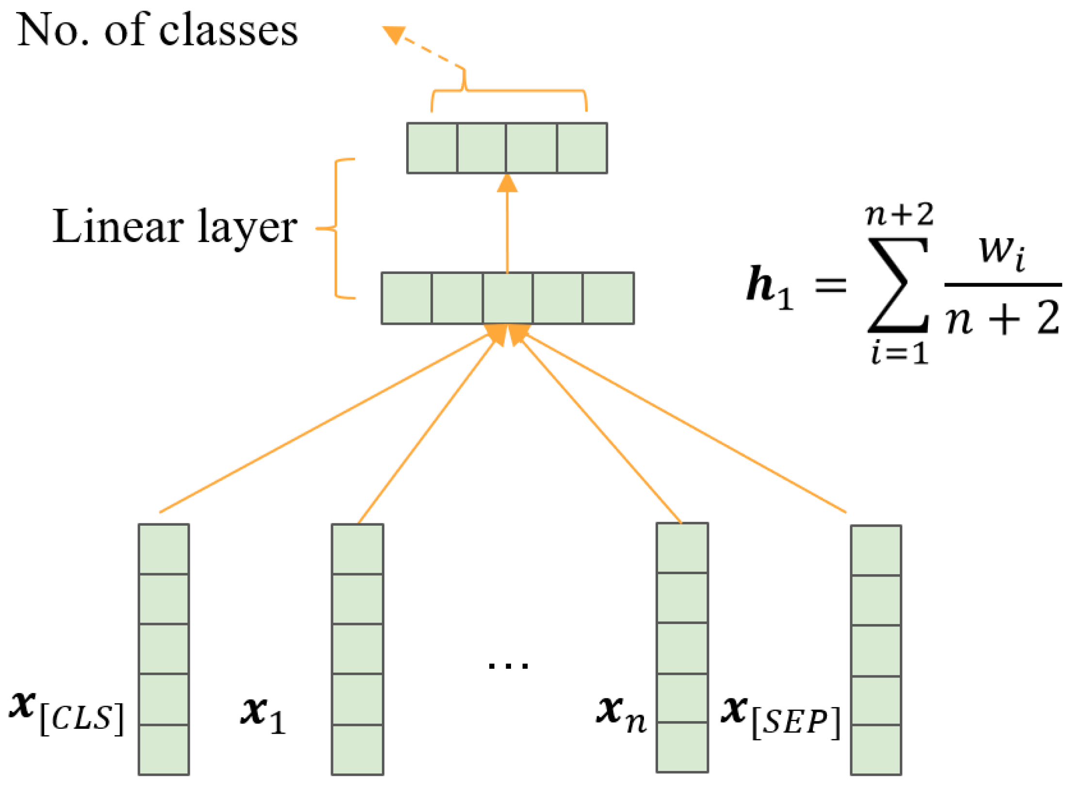
One of the simplest uses of the BERT architecture is baseBERT, which uses BERT for word embeddings and then feeds the vector representation of “[CLS]” into a linear layer classifier (see Figure 4).
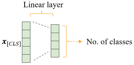
Figure 4.
The structure of base BERT in our work.
- (2)
- FFNN
FFNNs are the most primitive deep learning modes. A representative model is the deep average network (DAN) [65], as shown in Figure 5. Its main structure includes the embedded, average, linear, and output layers. In our work, we adopted the following structure depicted in Figure 5. The embedding size within our DAN was set to 100.
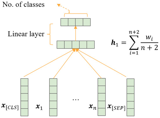
Figure 5.
DAN in our work.
- (3)
- CNN
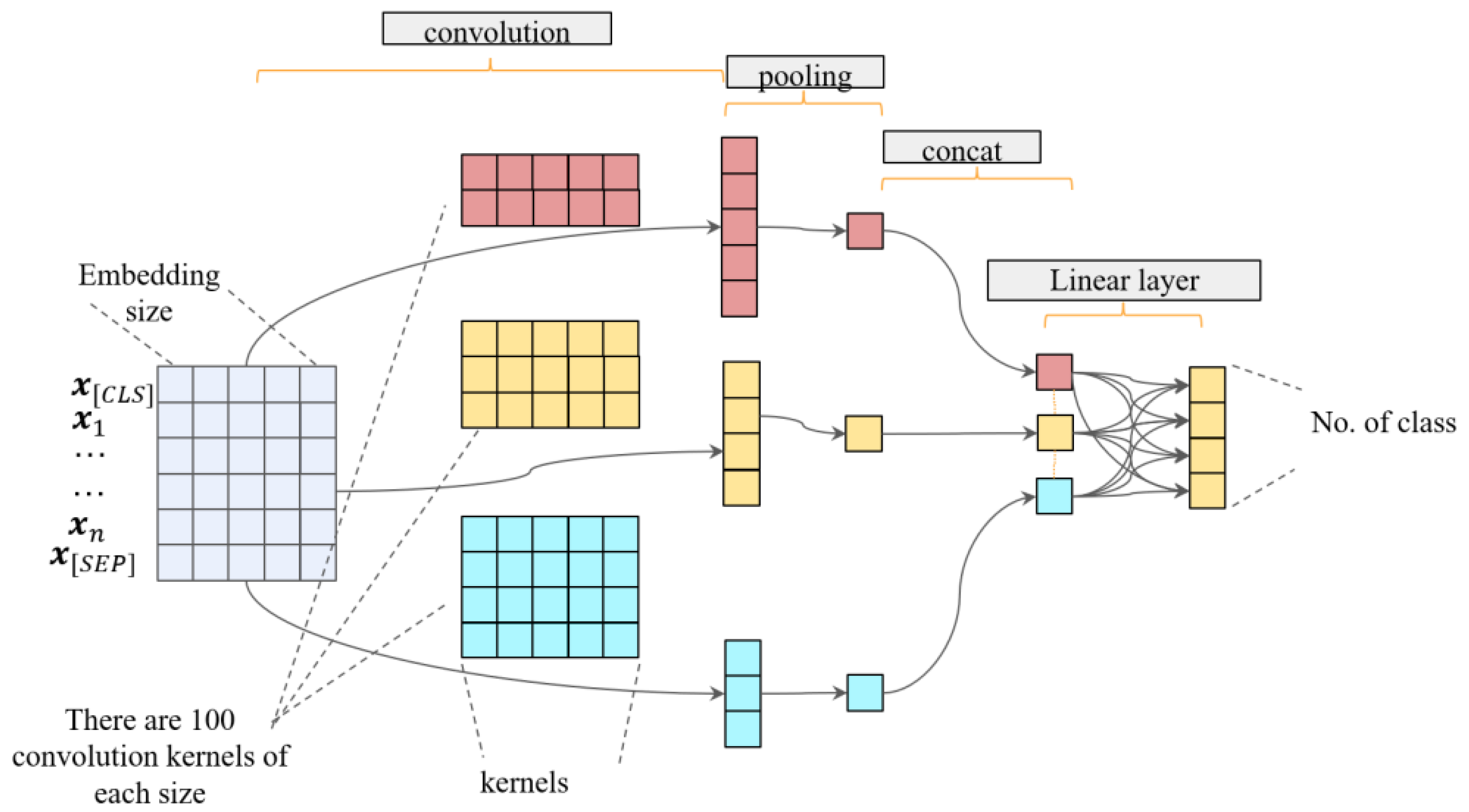
CNNs (convolutional neural networks) extract features from the input text by applying convolutional filters, enabling the capture of local n-gram patterns. Max-pooling layers then select the most important features, and fully connected layers classify the text. In our work, we used the structure based on the work of Kim [66]. We employed 100 kernels of three different sizes (2, 3, and 4) for feature extraction, followed by max-pooling for pooling (see Figure 6).

Figure 6.
CNN in our work.
- (4)
- LSTM
LSTM networks are a type of RNN designed to handle sequential data. In sentiment classification, LSTMs process text one token at a time, capturing contextual information through their memory cells. The final hidden state is then fed into a classification layer to predict the label. We used Bidirectional LSTM (BiLSTM) in our work (see Figure 7). The hidden layer size of the LSTM is 100 and the output size of the first linear layer is 128.
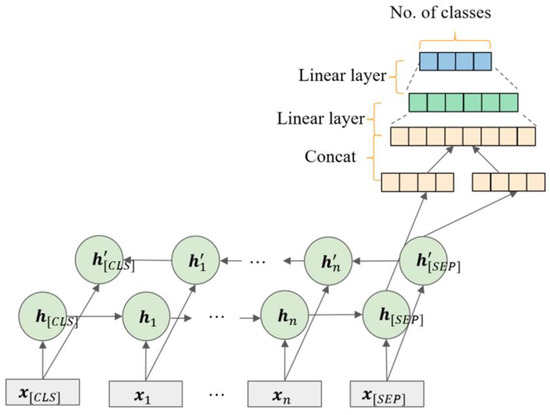
Figure 7.
LSTM in our work.
- (5)
- LSTM+attention
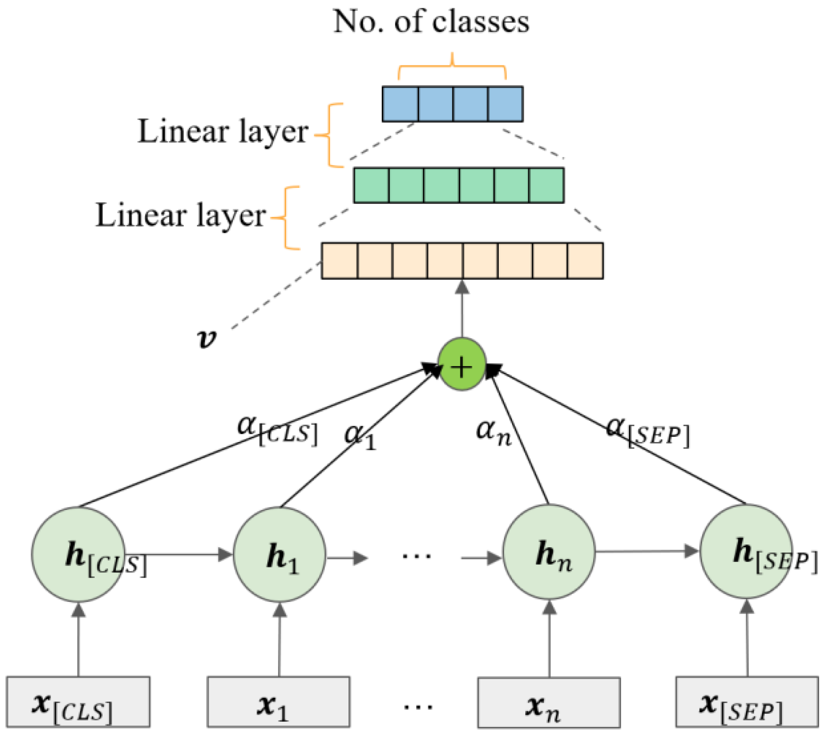
The ordinary LSTM-based text classification method only uses the output of the last time step as the input of the classifier, while the LSTM+attention-based method aims to weight the output of all time steps to obtain the input of the classifier (see Figure 8), which can consider more semantic information.

Figure 8.
LSTM+attention in our work.
We used the calculation of Yang et al. [67] to achieve as follows:
Then we can obtain the weighted sentence representation as follows:
where , , are parameters, is the weight of the output , and is the sentence representation after the weighted sum.
- (6)
- LSTM+CNN
The LSTM+CNN structure is able to combine the advantages of LSTM and CNN, where LSTM is able to capture long-term dependencies and CNN is able to extract local features. We added residual structure to help convergence. The model we used can be seen in Figure 9.
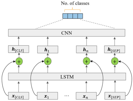
Figure 9.
LSTM+CNN in our work.
3.3.3. Output Layer
The output layer is unified as softmax layer for most deep-learning-based sentiment classification. The softmax layer can be calculated as follows:
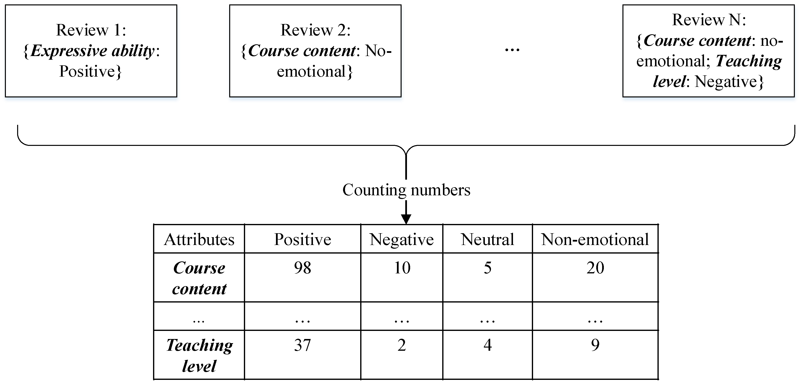
By utilizing our proposed sentiment classification method, we can extract the attributes mentioned in each review along with their corresponding sentiment. Subsequently, we calculate the overall count of reviews that involve distinct attributes and various emotional responses, as depicted in Figure 10.
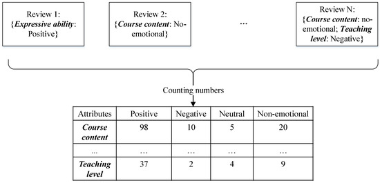
Figure 10.
An illustration of the total number of reviews involving different attributes and different emotions.
3.4. Determination Attributes Improvement Cost
For different course attributes of a course, it is difficult to obtain precise attribute improvement costs, but we can ask experts to judge the difficulty of different attributes to be improved and rank the difficulty. Given the difficulty rankings, we can use the rank sum weight method (RSW) to estimate the cost and obtain the proportion of each attribute improvement cost in the total cost. The RSW method is a method to determine attribute weights in MADM, which is able to generate quantitative weights of attributes based on the attribute importance ranking given by experts [68]. The proportion of each attribute improvement cost in the total cost can be calculated as follows:
In Formula (5), represents the improvement difficulty ranking of the th attribute; the more difficult it is, the higher the ranking. represents the total number of attributes. It is easy to see that in Formula (5), for all attributes, the denominator is a constant value, while the value of the numerator varies according to the ranking of the th attribute; the higher the ranking, the larger the numerator, and then the larger the proportion of the estimated cost.
3.5. Generation of the Priority of Attributes Improvement
After the previous steps, we obtained six evaluation criteria for each course attribute: the number of positive reviews (), the number of neutral reviews (), the number of negative reviews (), the number of non-emotional reviews (), the attribute frequency (), and the improvement cost () (see Table 1).

Table 1.
Evaluation matrix for all course attributes.
In Table 2, ,…, represent evaluation criteria, ,…, represent course attributes, and represents the value of the th evaluation criterion of the th attribute.

Table 2.
An example of attributes and attribute words.
Given the varying number of attribute words across different attributes, it is unfair to simply tally the total number of reviews expressing various sentiments for all the attribute words within a single attribute, especially for those with fewer attribute words. We normalize the values of , , , and using the number of reviews involving the attribute with positive, negative, neutral and no sentiment divided by the total number of reviews involving the attribute. For , we take the average of the number of reviews involving each word in an attribute.
So, we use the following formulas to calculate , , , , and :
can by calculated by Formula (5). In Formulas (6)–(10), represents the index of word, represents the set of attribute words for attribute , represents the cardinality of set , represents the number of reviews involving th word, represents the number of reviews involving any words in and , , , and represent the number of positive, neutral, negative, and non-emotional reviews involving th word, respectively.
Our task is to decide the priority of course attribute improvement. represents the degree of learners’ satisfaction. Obviously, the higher the degree of satisfaction, the lower the priority for improvement. Therefore, it is a cost criterion. The neutral reviews indicate that learners are not very satisfied with the mentioned attributes; that is, they still have a certain degree of dissatisfaction, and thus, is the benefit criterion. Similarly, is a benefit criterion. Although reviews without emotional content do not express satisfaction or dissatisfaction, if certain attributes are mentioned by learners in reviews, it means that learners may pay more attention to these attributes. Thus, the is benefit criterion. represents the total attention and is therefore a benefit criterion. The higher the improvement cost, the more difficult the improvement. Obviously, is the cost criterion.
Next, we employed the multi-attribute decision-making (MADM) approach to assess the attributes. Specifically, we utilized the Technique for Order Preference by Similarity to Ideal Solution (TOPSIS) method [69] to determine the priority scores for attribute improvement. TOPSIS determines a score for each alternative by calculating the distance between the true alternative and two ideal alternatives: the positive ideal alternative (a dummy alternative constructed with the best value of each attribute of all alternatives) and the negative ideal alternative (a dummy alternative constructed with the worst value of each attribute of all alternatives). The calculation process for TOPSIS has been detailed in our previous work [70].
The TOPSIS method requires the weights of various indicators to be determined beforehand. Therefore, we adopted the entropy weight method (EWM) to determine the weights of each indicator. Since the entropy weight method is an objective weight calculation method that determines the weight of an indicator based on the amount of information, it can reduce the deviation caused by subjective factors when determining the weight of indicators and make the results more practical. It has been widely used [71]. The calculation steps are as follows:
Step 1: Data standardization.
To eliminate the influence of varying scales and magnitudes, the original data must be normalized. The normalization formula is as follows:
where is the original value of the th evaluation criterion of the th alternative, is the normalized value, and and are the minimum and maximum values of the th evaluation criterion, respectively.
Step 2: Calculate the entropy value of each criterion.
Compute the entropy value for each criterion. The entropy value reflects the degree of dispersion in the criterion data. The formula is as follows:
where is the entropy value of the th evaluation criterion, is the number of alternatives, is the proportion of the th evaluation criterion value for the th alternative to the sum of that criterion, which can be calculated by , and is the natural logarithm.
Step 3: Calculate the dispersion coefficient of each criterion.
The dispersion coefficient is the reciprocal of the entropy value and reflects the ability of a criterion to distinguish between evaluation objects. The formula is as follows:
Step 4: Calculate the weight of each criterion.
Determine the weight for each criterion based on its dispersion coefficient. The weights are proportional to the dispersion coefficients. The formula is as follows:
where is the weight of the th evaluation criterion, and is the number of criteria.
4. Results
4.1. Data Collection and Preprocessing
As we said in Section 3.1, we used a Python crawler to crawl the review data from the Chinese University MOOC (https://www.icourse163.org/ (accessed on 1 February 2024)). As the largest online course platform in China, the Chinese University MOOC boasts a significant volume of reviews. We gathered reviews for two courses: C language and Java language, spanning from January 2018 to November 2022. The numbers of reviews for the two courses are 12,560 and 3980, respectively.
We then segmented the reviews by splitting the reviews with multiple sentences into a single sentence and filtering out those with sentences less than five characters in length. It should be noted that we added some turning words for sentence segmentation, such as “but” and “however”, because the text before and after these words often have different sentiments. Although some sentences were removed because they were less than five characters, some long reviews were split into multiple sentences, resulting in 11,327 and 3865 sentences, respectively.
Subsequently, we conducted part-of-speech (POS) tagging on both datasets, focusing on extracting nouns and their respective document frequencies. Document frequency refers to the count of review sentences in which a particular term appears. We then filter out words with too few document frequencies. Since the number of reviews in the two courses is different, it is not fair to filter words with the same criterion. Hence, for the C language course, we eliminated nouns with a document frequency of less than five, while for the Java language course, we excluded those with a document frequency of less than two. We manually weeded out nouns or noun phrases unrelated to the course content, such as “thank you”, “not interesting”, and “a waste of time”. Consequently, we arrived at 340 alternative attribute words for the C language course and 350 for the Java language course.
4.2. Course Attributes Extraction
As previously mentioned in Section 3.2, we implemented loading FastText word vectors and AP clustering in Python. We then filtered and reorganized the clustered results, resulting in 10 attributes for both courses. The original results are in Chinese; for the convenience of readers, we use the translation results of the original words as attribute words and show a part of the attribute words for each attribute (see Table 2). The complete results in Chinese are shown on github (https://github.com/yangpeiailong/Text-Mining-and-Multi-Attribute-Decision-Making-based-Course-Improvement-in-MOOCs/tree/main/mooc/data/1attributes (accessed on 10 February 2024)).
4.3. Determination of the Emotional and Non-Emotional Content Corresponding to the Course Attributes
As stated in Section 3.3, we intend to utilize deep learning for sentiment analysis. However, deep learning models require labeled samples for training. Therefore, we manually annotated a subset of samples selected from our collected dataset. To prevent a decline in training accuracy due to imbalanced data, we aim to maintain a similar number of samples across all classes during the labeling process. Consequently, apart from the reviews collected for the two courses, we also gathered feedback from other similar courses. Despite this, neutral reviews remain relatively scarce. Therefore, we can only ensure that the number of other classes of data is similar and the number of neutral reviews is relatively small. The training sample consisted of 572 positive, 125 neutral, 537 negative, and 531 emotionless comments, amounting to a total of 1765 comments.
Subsequently, we trained six deep-learning-based classifiers using these samples and evaluated their performance. The settings of our deep learning models are as follows:
- (1)
- Our deep learning models have been implemented using Pytorch 2.2.0 with a GTX 1080Ti graphics card and 32 GB of RAM.
- (2)
- The loss functions were the cross-entropy loss functions, and the gradient descent algorithm was adaptive motion estimation or stochastic gradient descent, with learning rates ranging from 1 × 10⁻¹ to 1 × 10⁻⁵.
- (3)
- The number of epochs is 40.
- (4)
- The numbers of training and test batches were 32 and 100, respectively.
- (5)
- The embedding word vector size of the BERT-based models was 768.
- (6)
- The pre-trained BERT model utilized was the BERTModel, in conjunction with the BERTTokenizer tools from the Hugging Face transformer toolkit. This toolkit provides a Pytorch interface, enabling training and utilization with various intermediate structures, all implemented using Pytorch.
- (7)
- We use accuracy to evaluate the performance of all six models, which can be calculated as follows:where represents the number of samples that are correctly classified, and represents the number of samples. To calculate the accuracy, we employed five-fold cross-validation, a technique that evaluates machine learning algorithms by dividing the available data into k equal-sized subsets. The model is trained k times, with k−1 subsets used for training and one subset reserved for validation. This iterative process ensures that each subset is utilized for validation once during the k iterations, thereby providing an unbiased assessment of the model’s performance. The source code is available at github (https://github.com/yangpeiailong/Text-Mining-and-Multi-Attribute-Decision-Making-based-Course-Improvement-in-MOOCs/tree/main/mooc/codes (accessed on 10 February 2024)). The accuracy of the six classifiers is shown in Figure 11.
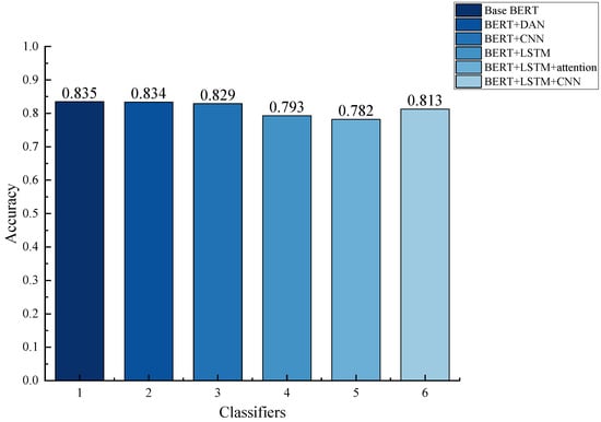 Figure 11. The accuracy of the six classifiers.
It is evident that base BERT exhibits superior performance among the six classifiers, making it the preferred choice for data labeling. Following the labeling process, we tallied the number of reviews expressing different sentiments for each attribute. These results are presented in Appendix A.
Appendix A reveals that across all attributes, the number of positive reviews consistently dominates, indicating a general satisfaction with the attributes of these two courses. Nevertheless, the extent of satisfaction exhibits considerable variation among different attributes. Notably, attributes such as “Teaching Level” and “Teaching Method” enjoy high satisfaction levels, with the combined count of neutral and negative reviews comprising less than one-third of the total. In contrast, attributes such as “Exercise” exhibit lower satisfaction levels, with neutral and negative reviews comprising nearly half of the total feedback. This underscores the varying degrees of satisfaction across different attributes.
4.4. Determination Attributes Improvement Cost
To minimize the risk of biased judgments resulting from reliance on a sole expert’s opinion, we disbursed the extracted attributes and corresponding attribute words to six experts for independent review. This approach guaranteed that each expert, leveraging their unique professional expertise, would base their judgments solely on their thorough comprehension of the attributes. Consequently, a more balanced and comprehensive evaluation of the cost of attribute improvement was achieved.
Since both courses belong to the programming category and share identical attributes, it is reasonable to presume that the cost of enhancing these attributes would be comparable. Therefore, in order to streamline the ranking process, we did not ask experts to individually rank each attribute for each course. Instead, we requested a unified ranking for the attributes across both courses. The resulting rankings are presented in Table 3.

Table 3.
The ranking results of improvement cost of all attributes.
Table 3 reveals that while there exist minor disparities in experts’ assessments regarding the cost of attribute improvement, the overall trend remains consistent. All experts agree that enhancing attributes such as “Teaching level”, “Course organization”, and “Professional knowledge” involves a relatively high cost. Conversely, attributes like “Teacher’s expressive ability”, “Exercise”, and “Supporting materials” are considered easier to improve.
This finding resonates strongly with our intuitive understanding. The enhancement of attributes such as teachers’ professional knowledge, teaching level, and course organization is deeply ingrained in their extensive learning and experience. Consequently, these aspects are inherently challenging to improve in the short term. In contrast, other attributes, which are not intrinsically tied to teachers, can be relatively easier to improve upon.
The calculation of Formula (5) requires a set of rankings, but our six experts have provided us with a total of six sets of rankings, which makes it impossible for us to directly bring the results of Table 3 into Formula (5) for calculation. Nonetheless, considering that there is little difference in the judgments of the experts, we directly calculate the averages of the rankings across six experts for each attribute and then bring it into Equation (5) to calculate the improvement cost.
4.5. Generation of the Priority of Attributes Improvement
Utilizing Equations (6)–(10) and the preceding results, we constructed the decision matrices for both courses, as presented in Table 4 and Table 5.

Table 4.
The decision matrix of C language.

Table 5.
The decision matrix of Java language.
Based on the results in Table 4 and Table 5, we can use Formulas (11)–(14) to calculate the criteria weights. Because our evaluation criteria include benefit and cost criteria, for cost criteria, we transform them into benefit criteria by calculating their reciprocals. The results are shown in Table 6.

Table 6.
The criteria weights of both courses.
Then, we can use TOPSIS to calculate the improvement priority score and ranking of each attribute of the two courses. The results are shown in Table 7.

Table 7.
The decision matrix of Java language.
5. Discussion
5.1. Single Criterion Analysis
We first analyzed the results in Table 4 and Table 5, which reflect the performance of the attributes of the two courses on the six criteria.
We first analyzed the three criteria , , and , which are the proportion of positive, neutral, and negative reviews among all learners’ comments on an attribute and directly reflect learners’ satisfaction with the attribute. For an attribute, the higher is, or the lower and are, the higher the learner’s satisfaction is; otherwise, the lower the satisfaction is. It is not difficult to find that for the two programming courses, there is little difference in the attribute satisfaction of learners for between the two courses. The two attributes that learners are most satisfied with are “Teaching level” and “Learning threshold”. The majority of the learners believed that the teachers in both courses possess a commendable level of expertise, and the courses were tailored to cater to beginners. The attributes that the learners felt performed well are “Teachers’ expressive ability”, “Teaching methods”, “Course organization” and “Learning experience”. It means that the teachers of these two courses have good expression ability, can basically tell the course content clearly, and adopt appropriate teaching methods. The schedule of the course is reasonable, and the key and difficult points are prominent. The learner’s listening experience was good. For “Supporting material”, Java language performs well, while C language performs moderately. For C, it may be necessary to provide more high-quality supporting material. The satisfaction of the “Platform” and “Professional knowledge” of the two courses is general, which means that learners are dissatisfied with the services provided by the MOOC platform to a certain extent, and the amount and depth of professional knowledge provided by the courses may need to be improved. Finally, learners expressed dissatisfaction with the “Exercise” aspect of both courses, indicating that there is ample room for improvement in terms of exercise difficulty and quantity.
We then analyzed . It is the proportion of non-emotional reviews for an attribute. As previously mentioned in Section 1, although non-emotional reviews do not directly reflect satisfaction or dissatisfaction, the attributes that reviewers mentioned in non-emotional reviews are the attributes that they thought might be of importance to future learners. It is evident that “Professional knowledge” is a relatively crucial attribute. A possible reason for this could be that in technical courses, learners tend to prioritize the quantity and quality of professional knowledge imparted by the instructor. Additionally, the expression of professional knowledge in reviews tends to utilize more non-emotional descriptions. This does not imply that other attributes are less significant; however, they may be more easily expressed through emotional reviews.
For , it is the average of the number of reviews involving each word in an attribute. A higher value of means that people pay more attention to the attribute word in this attribute and, accordingly, pay more attention to this attribute. Learners of both courses pay significant attention to attributes such as “Teaching level”, “Learning threshold”, “Course organization”, and “Teacher’s expressive ability”. These four attributes directly influence the learning effectiveness of students. Hence, this finding aligns with our intuitive understanding. “Professional knowledge” and “Platform” are of much interest in C language but not so much in Java. This divergence might be attributed to the widespread perception of C as a programming language closer to hardware, distinguished by its low-level and intricate syntax and structure. Consequently, learners often require a deeper level of proficiency and educational guidance to comprehend and utilize it effectively. On the contrary, Java’s more refined and straightforward syntax may not necessitate extensive expertise, particularly for novice learners. The remaining attributes are of lesser concern to learners. The potential reason is that these attributes may have a minimal impact on the learning outcomes and may not hold significant value for future learners, as perceived by those who have already completed the learning process.
has already been discussed in Section 4.4, so we will not add anything further.
5.2. Comprehensive Analysis
We then analyzed the results in Table 7, which reflect the comprehensive performance of the attributes of the two courses.
We began our analysis with the top-ranked attributes: “Exercise”, “Teaching level”, “Professional knowledge”, and “Platform”. Among these, “Exercise” receives the lowest satisfaction rating and is relatively inexpensive to improve, thus carrying the highest priority. For “Teaching level”, although it has the highest satisfaction and improvement cost, it still has a high improvement priority because it is the attribute that learners pay the most attention to. For “Professional knowledge”, despite its low attention and high improvement cost, it still has a high improvement priority because of its low satisfaction. For “Platform”, although it does not have high attention, it has low improvement cost and low satisfaction, so it has high priority.
Next, we analyzed the attributes that are in the middle ranking: “Teacher’s expressive ability” and “Supporting materials”. For “Teacher’s expressive ability” and “Supporting materials”, although their improvements are less costly, they have medium satisfaction, medium attention, and therefore medium improvement priorities.
Finally, we delved into the lower-ranked attributes: “Course organization”, “Experience of learning”, “Teaching method”, and “Learning threshold”. “Course organization” and “Experience of learning” carry low improvement priority due to their medium satisfaction ratings, low attention levels, and high costs of improvement. For “Teaching method”, since they have high satisfaction, low attention, and a medium cost of improvement, they have a low priority for improvement. For “Learning threshold”, despite its high attention, it has low priority for improvement due to its high satisfaction and high cost of improvement.
Following the aforementioned analysis, our method is capable of comprehensively taking into account various facets of improving course attributes, thereby encouraging a more comprehensive approach when contemplating improvements to MOOCs.
5.3. Implications and Future Research
The limitations of this study and potential future research avenues primarily encompass the following aspects: Firstly, a sentiment analysis might not be sufficiently precise. The sentence-level sentiment analysis method we employed assumes that the sentiment expressed in a sentence corresponds to the attributes mentioned within it. However, this approach can be limited when a sentence contains multiple attributes and varying emotions. Future research should focus on employing more fine-grained sentiment analysis methods, such as aspect-level sentiment analysis, to enhance the precision of sentiment analysis. Second, the way we determine costs is not necessarily accurate. As our attribute improvement costs are determined through the voting of six experts, this sample size may not be sufficient and introduces a degree of subjectivity, potentially leading to inaccuracies in cost judgments. Therefore, a comprehensive and thorough investigation into the costs associated with course improvements is crucial. Thirdly, we have employed only one method for multi-attribute decision-making, namely TOPSIS. However, there may be other, more suitable methods available. It is imperative to explore and discuss whether other multiple-attribute decision-making techniques might outperform TOPSIS in certain scenarios. Fourthly, our experiments were limited to only two courses: C language and Java language. Consequently, the experimental results obtained may not be universally applicable. To validate the generalizability of our method, it is necessary to apply it to courses across diverse fields.
6. Conclusions
Based on the learner’s perspective, this paper presents a method that leverages text mining and multi-attribute decision-making frameworks to enhance the attributes of MOOCs, taking into account both non-emotional reviews and improvement costs. Initially, the method collected online reviews from MOOC platforms and extracted pertinent course attributes from these reviews. Subsequently, the review text was categorized into four sentiment groups—positive, neutral, negative, and non-emotional—utilizing deep learning techniques. To ascertain the improvement costs associated with each attribute, an expert voting mechanism was utilized. Finally, a decision matrix was constructed, and the TOPSIS method was employed to prioritize the attributes for improvement. To validate the effectiveness of our proposed method, it was applied to two programming courses: C language and Java language. The experimental results demonstrate the utility of our approach. The main contributions of this study are as follows:
- (1)
- Regarding data selection, this study employed learners’ online comments as the analytical dataset to establish a text mining model specifically tailored for MOOC online comments. The outcomes offer a real-time and visual representation of learners’ preferences and needs.
- (2)
- Given the limited resources available, realizing their rational utilization holds significant importance in enhancing the overall quality of courses. Previous studies have primarily focused on determining the priority of attribute improvements solely based on learners’ satisfaction levels, neglecting the crucial aspect of cost. Nevertheless, cost plays a pivotal role in the improvement process of course attributes. In scenarios where the cost of enhancing a specific attribute is prohibitively high, it becomes imperative to deliberate on whether to pursue such improvements despite their low satisfaction rating. Consequently, this study builds upon previous research, incorporating both cost considerations and non-emotional reviews, thereby enabling course managers to undertake a more comprehensive evaluation when aiming to enhance courses.
- (3)
- This study introduces a novel approach that integrates text mining and multi-attribute decision-making frameworks to effectively enhance MOOC attributes from the learners’ perspective. By incorporating non-emotional reviews and considering improvement costs, our method offers a comprehensive and practical solution to course managers. The utilization of deep learning techniques in sentiment analysis ensures accurate categorization of reviews, while the expert voting mechanism provides a reliable estimation of improvement costs. The TOPSIS method then facilitates the prioritization of attributes for improvement, enabling course managers to make informed decisions. This approach not only addresses the challenges associated with managing overwhelming information but also ensures that limited resources are allocated efficiently.
- (4)
- Overall, at the theoretical level, this study contributes to enriching relevant research on MOOC improvement by adopting a learner-centric perspective. It also serves as a valuable reference for similar studies. From a managerial perspective, the utilization of text mining and multi-attribute decision-making techniques enables a more precise analysis of curriculum attributes, thus addressing the challenge of managing overwhelming information faced by course managers. Furthermore, it offers course managers a more comprehensive framework to prioritize the improvement of course attributes across six dimensions: positive emotion, neutral emotion, negative emotion, no emotion, attention, and cost.
Author Contributions
Methodology, P.Y.; writing—original draft, P.Y.; visualization, P.Y.; Writing—review and editing, Y.L. (Ying Liu) and Z.W.; investigation, Y.L. (Ying Liu) and X.C.; formal analysis, Y.L. (Yuyan Luo), Z.W. and X.C.; supervision, Y.L. (Yuyan Luo). All authors have read and agreed to the published version of the manuscript.
Funding
This research was funded by the Higher Education Scientific Research Planning Project in 2022 of Chinese Association of Higher Education (Grant No. 22CX0406), the Ideological and Political Education Research Project in 2023 of University Ideological and Political Work Team Training and Research Center (Grant No. CJSFZ23-33), and the Key Research Base of Humanities and Social Sciences of Sichuan Province-Sichuan Education Informatization Application and Development Research Center Project (Project No. JYXX20-004). Major Projects on Talent Cultivation and Teaching Reform in Higher Education in Sichuan Province in 2023 (JG2023-49). The General Project of Graduate Education and Teaching Reform in Chengdu University of Technology (Grant No. 2023YJG203).
Institutional Review Board Statement
Not applicable.
Informed Consent Statement
Not applicable.
Data Availability Statement
The data presented in this study are available on request from the corresponding authors.
Conflicts of Interest
The authors declare no conflicts of interest.
Appendix A

Table A1.
The number of reviews in different sentiments for each attribute for C language.
Table A1.
The number of reviews in different sentiments for each attribute for C language.
| Attributes | Positive | Neutral | Negative | Non-Emotional |
|---|---|---|---|---|
| Teacher’s expressive ability | 284 | 18 | 27 | 76 |
| Teaching level | 4278 | 177 | 159 | 313 |
| Teaching method | 428 | 29 | 37 | 58 |
| Exercise | 224 | 55 | 174 | 26 |
| Learning threshold | 1382 | 62 | 74 | 150 |
| Course organization | 2199 | 135 | 353 | 230 |
| Supporting materials | 193 | 26 | 62 | 20 |
| Platform | 273 | 30 | 85 | 52 |
| Experience of learning | 851 | 70 | 168 | 101 |
| Professional knowledge | 611 | 52 | 135 | 214 |

Table A2.
The number of reviews in different sentiments for each attribute for Java language.
Table A2.
The number of reviews in different sentiments for each attribute for Java language.
| Attributes | Positive | Neutral | Negative | Non-Emotional |
|---|---|---|---|---|
| Teacher’s expressive ability | 113 | 13 | 9 | 15 |
| Teaching level | 1682 | 80 | 68 | 150 |
| Teaching method | 156 | 15 | 16 | 17 |
| Exercise | 62 | 22 | 81 | 11 |
| Learning threshold | 558 | 28 | 28 | 43 |
| Course organization | 823 | 66 | 124 | 106 |
| Supporting materials | 90 | 5 | 17 | 9 |
| Platform | 68 | 7 | 21 | 8 |
| Experience of learning | 329 | 25 | 54 | 33 |
| Professional knowledge | 185 | 27 | 37 | 69 |
References
- Ahmadi, S.; Nourmohamadzadeh, Z.; Amiri, B. A hybrid DEMATEL and social network analysis model to identify factors affecting learners’ satisfaction with MOOCs. Heliyon 2023, 9, e17894. [Google Scholar] [CrossRef]
- Huang, H.; Jew, L.; Qi, D.D. Take a MOOC and then drop: A systematic review of MOOC engagement pattern and dropout factor. Heliyon 2023, 9, e15220. [Google Scholar] [CrossRef]
- Zhang, C.H.; Su, W.H.; Chen, S.C.; Zeng, S.Z.; Liao, H.C. A Combined Weighting Based Large Scale Group Decision Making Framework for MOOC Group Recommendation. Group Decis. Negot. 2023, 32, 537–567. [Google Scholar] [CrossRef]
- Ossiannilsson, E.; Altınay, Z.; Altınay, F. Towards fostering quality in open online education through OER and MOOC practices. In Open Education: From OERs to MOOCs; Springer: Berlin, Heidelberg, Germany, 2017; pp. 189–204. [Google Scholar]
- Guerrero, M.; Heaton, S.; Urbano, D. Building universities’ intrapreneurial capabilities in the digital era: The role and impacts of Massive Open Online Courses (MOOCs). Technovation 2021, 99, 102139. [Google Scholar] [CrossRef]
- Li, L.; Johnson, J.; Aarhus, W.; Shah, D. Key factors in MOOC pedagogy based on NLP sentiment analysis of learner reviews: What makes a hit. Comput. Educ. 2022, 176, 104354. [Google Scholar] [CrossRef]
- Su, B.H.; Peng, J. Sentiment Analysis of Comment Texts on Online Courses Based on Hierarchical Attention Mechanism. Appl. Sci. 2023, 13, 4204. [Google Scholar] [CrossRef]
- Castillo, N.M.; Lee, J.; Zahra, F.T.; Wagner, D.A. MOOCS for development: Trends, challenges, and opportunities. Int. Technol. Int. Dev. 2015, 11, 35–42. [Google Scholar]
- Gomez, M.J.; Calderón, M.; Sánchez, V.; Clemente, F.J.G.; Ruipérez-Valiente, J.A. Large scale analysis of open MOOC reviews to support learners’ course selection. Expert Syst. Appl. 2022, 210, 118400. [Google Scholar] [CrossRef]
- Talebi, K.; Torabi, Z.; Daneshpour, N. Ensemble models based on CNN and LSTM for dropout prediction in MOOC. Expert Syst. Appl. 2024, 235, 121187. [Google Scholar] [CrossRef]
- Li, S.; Du, J.L.; Yu, S. Diversified resource access paths in MOOCs: Insights from network analysis. Comput. Educ. 2023, 204, 104869. [Google Scholar] [CrossRef]
- Pandey, M.; Litoriya, R.; Pandey, P. Scrutinizing student dropout issues in MOOCs using an intuitionistic fuzzy decision support system. J. Intell. Fuzzy Syst. 2023, 44, 4041–4058. [Google Scholar] [CrossRef]
- Wang, Y. Where and what to improve? Design and application of a MOOC evaluation framework based on effective teaching practices. Distance Educ. 2023, 44, 458–475. [Google Scholar] [CrossRef]
- Almufarreh, A.; Arshad, M. Exploratory Students’ Behavior towards Massive Open Online Courses: A Structural Equation Modeling Approach. Systems 2023, 11, 223. [Google Scholar] [CrossRef]
- Qi, C.; Liu, S.D. Evaluating On-Line Courses via Reviews Mining. IEEE Access 2021, 9, 35439–35451. [Google Scholar] [CrossRef]
- Wei, X.X.; Taecharungroj, V. How to improve learning experience in MOOCs an analysis of online reviews of business courses on Coursera. Int. J. Manag. Educ. 2022, 20, 100675. [Google Scholar] [CrossRef]
- Ahadi, A.; Singh, A.; Bower, M.; Garrett, M. Text mining in education—A bibliometrics-based systematic review. Educ. Sci. 2022, 12, 210. [Google Scholar] [CrossRef]
- Geng, S.; Niu, B.; Feng, Y.; Huang, M. Understanding the focal points and sentiment of learners in MOOC reviews: A machine learning and SC-LIWC-based approach. Br. J. Educ. Technol. 2020, 51, 1785–1803. [Google Scholar] [CrossRef]
- Liu, Q.; Ding, Y.; Qian, P.; Li, R.; Zhou, J. Analysis of the influencing factors of online classes satisfaction based on text mining Take MOOC platform art education online classes as an example. J. Educ. Humanit. Soc. Sci. 2022, 2, 249–256. [Google Scholar] [CrossRef]
- Jung, H.; Lee, B.G. Research trends in text mining: Semantic network and main path analysis of selected journals. Expert Syst. Appl. 2020, 162, 113851. [Google Scholar] [CrossRef]
- Kou, G.; Yang, P.; Peng, Y.; Xiao, H.; Xiao, F.; Chen, Y.; Alsaadi, F.E. A cross-platform market structure analysis method using online product reviews. Technol. Econ. Dev. Econ. 2021, 27, 992–1018. [Google Scholar] [CrossRef]
- Chen, K.; Jin, J.; Luo, J. Big consumer opinion data understanding for Kano categorization in new product development. J. Ambient. Intell. Humaniz. Comput. 2022, 13, 2269–2288. [Google Scholar] [CrossRef]
- Shi, L.L.; Lin, J.; Liu, G.Q. Product feature extraction from Chinese online reviews: Application to product improvement. Rairo-Oper. Res. 2023, 57, 1125–1147. [Google Scholar] [CrossRef]
- Zhou, F.; Ayoub, J.; Xu, Q.; Yang, X.J. A machine learning approach to customer needs analysis for product ecosystems. J. Mech. Des. 2020, 142, 011101. [Google Scholar] [CrossRef]
- Lee, H.; Cha, M.S.; Kim, T. Text mining-based mapping for kano quality factor. ICIC Express Letters. Part B, Applications: An International. J. Res. Surv. 2021, 12, 185–191. [Google Scholar]
- Guo, J.; Wang, X.; Wu, Y. Positive emotion bias: Role of emotional content from online customer reviews in purchase decisions. J. Retail. Consum. Serv. 2020, 52, 101891. [Google Scholar] [CrossRef]
- Picazo-Vela, S.; Chou, S.Y.; Melcher, A.J.; Pearson, J.M. Why provide an online review? An extended theory of planned behavior and the role of Big-Five personality traits. Comput. Hum. Behav. 2010, 26, 685–696. [Google Scholar] [CrossRef]
- Li, G.; Reimann, M.; Zhang, W. When remanufacturing meets product quality improvement: The impact of production cost. Eur. J. Oper. Res. 2018, 271, 913–925. [Google Scholar] [CrossRef]
- Zavadskas, E.K.; Turskis, Z.; Kildienė, S. State of art surveys of overviews on MCDM/MADM methods. Technol. Econ. Dev. Econ. 2014, 20, 165–179. [Google Scholar] [CrossRef]
- Kastrati, Z.; Imran, A.S.; Kurti, A. Weakly supervised framework for aspect-based sentiment analysis on students’ reviews of MOOCs. IEEE Access 2020, 8, 106799–106810. [Google Scholar] [CrossRef]
- Mrhar, K.; Benhiba, L.; Bourekkache, S.; Abik, M. A Bayesian CNN-LSTM model for sentiment analysis in massive open online courses MOOCs. Int. J. Emerg. Technol. Learn. 2021, 16, 216–232. [Google Scholar] [CrossRef]
- Wang, C.; Huang, S.; Zhou, Y. Sentiment analysis of MOOC reviews via ALBERT-BiLSTM model. EDP Sci. 2021, 336, 05008. [Google Scholar] [CrossRef]
- Dina, N.; Yunardi, R.; Firdaus, A. Utilizing text mining and feature-sentiment-pairs to support data-driven design automation massive open online course. Int. J. Emerg. Technol. Learn. 2021, 16, 134–151. [Google Scholar] [CrossRef]
- Liu, W.; Lin, S.; Gao, B.; Huang, K.; Liu, W.; Huang, Z.; Feng, J.; Chen, X.; Huang, F. BERT-POS: Sentiment analysis of MOOC reviews based on BERT with part-of-speech information. In Proceedings of the 23rd International Conference on Artificial Intelligence in Education, Durham, UK, 27–31 July 2022; Springer International Publishing: Cham, Switzerland, 2022; pp. 371–374. [Google Scholar]
- Liu, Z.; Kong, X.; Chen, H.; Liu, S.; Yang, Z.K. MOOC-BERT: Automatically Identifying Learner Cognitive Presence from MOOC Discussion Data. IEEE Trans. Learn. Technol. 2023, 16, 528–542. [Google Scholar] [CrossRef]
- Lundqvist, K.; Liyanagunawardena, T.; Starkey, L. Evaluation of student feedback within a MOOC using sentiment analysis and target groups. Int. Rev. Res. Open Distrib. Learn. 2020, 21, 140–156. [Google Scholar] [CrossRef]
- Hew, K.F.; Hu, X.; Qiao, C.; Tang, Y. What predicts student satisfaction with MOOCs: A gradient boosting trees supervised machine learning and sentiment analysis approach. Comput. Educ. 2020, 145, 103724. [Google Scholar] [CrossRef]
- Nie, Y.; Luo, H.; Sun, D. Design and validation of a diagnostic MOOC evaluation method combining AHP and text mining algorithms. Interact. Learn. Environ. 2021, 29, 315–328. [Google Scholar] [CrossRef]
- Chen, X.; Cheng, G.; Xie, H.; Chen, G.; Zou, D. Understanding MOOC reviews: Text mining using structural topic model. Hum.-Cent. Intell. Syst. 2021, 1, 55–56. [Google Scholar] [CrossRef]
- Nilashi, M.; Abumalloh, R.A.; Zibarzani, M.; Samad, S.; Zogaan, W.A.; Ismail, M.Y.; Mohd, S.; Akib, N.A.M. What factors influence students satisfaction in massive open online courses? Findings from user-generated content using educational data mining. Educ. Inf. Technol. 2022, 27, 9401–9435. [Google Scholar] [CrossRef]
- Wang, W.; Liu, H.W.; Wu, Y.J.; Goh, M. Disconfirmation effect on online reviews and learner satisfaction determinants in MOOCs. Educ. Inf. Technol. 2023, 28, 15497–15521. [Google Scholar] [CrossRef]
- Blei, D.M.; Ng, A.Y.; Jordan, M.I. Latent dirichlet allocation. J. Mach. Learn. Res. 2003, 3, 993–1022. [Google Scholar]
- Liu, C.; Jia, G.; Kong, J. Requirement-oriented engineering characteristic identification for a sustainable product–service system: A multi-method approach. Sustainability 2020, 12, 8880. [Google Scholar] [CrossRef]
- Chen, Z.S.; Liu, X.L.; Chin, K.S.; Pedrycz, W.; Tsui, K.L.; Skibniewski, M.J. Online-review analysis based large-scale group decision-making for determining passenger demands and evaluating passenger satisfaction: Case study of high-speed rail system in China. Inf. Fusion 2021, 69, 22–39. [Google Scholar] [CrossRef]
- Jin, J.; Jia, D.; Chen, K. Mining online reviews with a Kansei-integrated Kano model for innovative product design. Int. J. Prod. Res. 2022, 60, 6708–6727. [Google Scholar] [CrossRef]
- Goldberg, D.M.; Abrahams, A.S. Sourcing product innovation intelligence from online reviews. Decis. Support Syst. 2022, 157, 113751. [Google Scholar] [CrossRef]
- Huang, S.; Zhang, J.; Yang, C.; Gu, Q.; Li, M.; Wang, W. The interval grey QFD method for new product development: Integrate with LDA topic model to analyze online reviews. Eng. Appl. Artif. Intell. 2022, 114, 105213. [Google Scholar] [CrossRef]
- Ji, F.; Cao, Q.; Li, H.; Fujita, H.; Liang, C.; Wu, J. An online reviews-driven large-scale group decision making approach for evaluating user satisfaction of sharing accommodation. Expert Syst. Appl. 2023, 213, 118875. [Google Scholar] [CrossRef]
- Joung, J.; Kim, H. Interpretable machine learning-based approach for customer segmentation for new product development from online product reviews. Int. J. Inf. Manag. 2023, 70, 102641. [Google Scholar] [CrossRef]
- Zhang, F.; Song, W. Product improvement in a big data environment: A novel method based on text mining and large group decision making. Expert Syst. Appl. 2024, 245, 123015. [Google Scholar] [CrossRef]
- Liang, X.; Liu, P.D.; Wang, Z.H. Hotel selection utilizing online reviews: A novel decision support model based on sentiment analysis and dl-vikor method. Technol. Econ. Dev. Econ. 2019, 25, 1139–1161. [Google Scholar] [CrossRef]
- Lenort, R.; Wicher, P.; Zapletal, F. On influencing factors for Sustainable Development goal prioritisation in the automotive industry. J. Clean Prod. 2023, 387, 135718. [Google Scholar] [CrossRef]
- Cao, P.P.; Zheng, J.; Li, M.Y. Product Selection Considering Multiple Consumers’ Expectations and Online Reviews: A Method Based on Intuitionistic Fuzzy Soft Sets and TODIM. Mathematics 2023, 11, 3767. [Google Scholar] [CrossRef]
- Vyas, V.; Uma, V.; Ravi, K. Aspect-based approach to measure performance of financial services using voice of customer. J. King Saud Univ.-Comput. Inf. Sci. 2022, 34, 2262–2270. [Google Scholar] [CrossRef]
- Li, K.; Chen, C.Y.; Zhang, Z.L. Mining online reviews for ranking products: A novel method based on multiple classifiers and interval-valued intuitionistic fuzzy TOPSIS. Appl. Soft. Comput. 2023, 139, 110237. [Google Scholar] [CrossRef]
- Qin, J.D.; Zeng, M.Z. An integrated method for product ranking through online reviews based on evidential reasoning theory and stochastic dominance. Inf. Sci. 2022, 612, 37–61. [Google Scholar] [CrossRef]
- Zhang, Z.Y.; Guo, J.; Zhang, H.R.; Zhou, L.X.; Wang, M.J. Product selection based on sentiment analysis of online reviews: An intuitionistic fuzzy TODIM method. Complex Intell. Syst. 2022, 8, 3349–3362. [Google Scholar] [CrossRef]
- Nilashi, M.; Mardani, A.; Liao, H.C.; Ahmadi, H.; Manaf, A.A.; Almukadi, W. A Hybrid Method with TOPSIS and Machine Learning Techniques for Sustainable Development of Green Hotels Considering Online Reviews. Sustainability 2019, 11, 6013. [Google Scholar] [CrossRef]
- Zayat, W.; Kilic, H.S.; Yalcin, A.S.; Zaim, S.; Delen, D. Application of MADM methods in Industry 4.0: A literature review. Comput. Ind. Eng. 2023, 177, 109075. [Google Scholar] [CrossRef]
- Behzadian, M.; Otaghsara, S.K.; Yazdani, M.; Ignatius, J. A state-of the-art survey of TOPSIS applications. Expert Syst. Appl. 2012, 39, 13051–13069. [Google Scholar] [CrossRef]
- Liu, Y.; Bi, J.W.; Fan, Z.P. A Method for Ranking Products through Online Reviews Based on Sentiment Classification and Interval-Valued Intuitionistic Fuzzy TOPSIS. Int. J. Inf. Technol. Decis. Mak. 2017, 16, 1497–1522. [Google Scholar] [CrossRef]
- Bojanowski, P.; Grave, E.; Joulin, A.; Mikolov, T. Enriching word vectors with subword information. Trans. Assoc. Comput. Linguist. 2017, 5, 135–146. [Google Scholar] [CrossRef]
- Frey, B.J.; Dueck, D. Clustering by passing messages between data points. Science 2007, 315, 972–976. [Google Scholar] [CrossRef] [PubMed]
- Devlin, J.; Chang, M.W.; Lee, K.; Toutanova, K. Bert: Pre-training of deep bidirectional transformers for language understanding. arXiv 2018, arXiv:1810.04805. [Google Scholar]
- Iyyer, M.; Manjunatha, V.; Boyd-Graber, J.; Daumé, H. Deep Unordered Composition Rivals Syntactic Methods for Text Classification. In Proceedings of the 53rd Annual Meeting of the Association for Computational Linguistics and the 7th International Joint Conference on Natural Language Processing, Beijing, China, 26–31 July 2015; Association for Computational Linguistics: Toronto, ON, Canada, 2015; Volume 1: Long Papers, pp. 1681–1691. [Google Scholar]
- Kim, Y. Convolutional neural networks for sentence classification. arXiv 2014, arXiv:1408.5882. [Google Scholar]
- Yang, Z.; Yang, D.; Dyer, C.; He, X.; Smola, A.; Hovy, E. Hierarchical attention networks for document classification. In Proceedings of the 2016 Conference of the North American Chapter of the Association for Computational Linguistics: Human Language Technologies, San Diego, CA, USA, 12–17 June 2016; pp. 1480–1489. [Google Scholar]
- Stillwell, W.G.; Seaver, D.A.; Edwards, W. A comparison of weight approximation techniques in multiattribute utility decision making. Organ. Behav. Hum. Perform. 1981, 28, 62–77. [Google Scholar] [CrossRef]
- Khan, M.N.; Gupta, N.; Matharu, M.; Khan, M.F. Sustainable E-Service Quality in Tourism: Drivers Evaluation Using AHP-TOPSIS Technique. Sustainability 2023, 15, 7534. [Google Scholar] [CrossRef]
- Kou, G.; Yang, P.; Peng, Y.; Xiao, F.; Chen, Y.; Alsaadi, F.E. Evaluation of feature selection methods for text classification with small datasets using multiple criteria decision-making methods. Appl. Soft Comput. 2020, 86, 105836. [Google Scholar] [CrossRef]
- Ji, J.; Wang, D.Y. Evaluation analysis and strategy selection in urban flood resilience based on EWM-TOPSIS method and graph model. J. Clean Prod. 2023, 425, 138955. [Google Scholar] [CrossRef]
Disclaimer/Publisher’s Note: The statements, opinions and data contained in all publications are solely those of the individual author(s) and contributor(s) and not of MDPI and/or the editor(s). MDPI and/or the editor(s) disclaim responsibility for any injury to people or property resulting from any ideas, methods, instructions or products referred to in the content. |
© 2024 by the authors. Licensee MDPI, Basel, Switzerland. This article is an open access article distributed under the terms and conditions of the Creative Commons Attribution (CC BY) license (https://creativecommons.org/licenses/by/4.0/).


