1. Introduction
Belt conveyors account for 30% of the total installed power of coal mines and consume 60% of the energy in coal mining operations, making them the main energy consuming equipment in coal mines [
1]. One approach to reduce energy consumption is to intelligently monitor and adjust the operating status of belt conveyors. Another strategy involves fundamentally reducing energy consumption through design and manufacturing improvements aimed at enhancing machine performance and reducing operating resistance. Under stable operation, the operating resistance of a belt conveyor mainly comprises the following components: main resistance, additional resistance, special resistance, and lifting resistance [
2]. The main resistance of the conveyor encompasses the rotational resistance of the rollers, the indentation rolling resistance generated by the relative movement between the conveyor belt and the rollers, and the bending resistance produced when the conveyor belt repeatedly bends under the action of the driving roller [
3].
The proportion of indentation rolling resistance exceeds half of the overall operating resistance [
4]. This resistance is generated by the rolling of a rigid roller on the surface of a viscoelastic material, such as the conveyor belt cover surface. The process of deformation and recovery of viscoelastic materials occurs gradually over time, leading to strain lagging behind stress [
5]. When a rigid cylinder rolls on the surface of a viscoelastic material, the contact area between the conveyor belt and the roller is asymmetric relative to the center of the roller. This results in an asymmetric distribution of the contact stress, generating resistance that hinders the movement of the conveyor belt, known as collapse rolling resistance [
6]. When the transportation distance of the belt conveyor is increased, it requires more rollers to support its weight, leading to a greater accumulation of collapse rolling resistance [
7]. In summary, the formation of indentation rolling resistance is attributed to the inherent characteristics of the material. Therefore, it is imperative to explore the characterization method of viscoelastic materials using the relaxation model (relaxation modulus function) and evaluate the relationship between the model and the indentation rolling resistance. The Maxwell model is used to characterize the viscoelastic properties of materials and establish the relaxation modulus function. However, the three-element Maxwell model, commonly used as an engineering characterization method, can only roughly provide an approximate characterization of the materials [
8]. In practical scenarios, material structures are more intricate, rendering the three-element model too simple to characterize them. The generalized Maxwell model, a theoretical representation method, offers a more comprehensive characterization of the viscoelasticity of materials [
9]. However, its applicability is limited by the actual testing time range. In this study, we address this limitation by modifying and streamlining the generalized Maxwell model. Subsequently, the model is integrated into the collapse rolling resistance formula to evaluate the collapse rolling resistance.
2. Related Studies
Wheeler and Munzenberger (2008) assessed indentation rolling resistance using the finite element analysis method [
10]. In addition, these scholars conducted experimental research to explore the indentation rolling resistance between the steel core conveyor belt and the roller using a testing device obtained from the University of New Zealand in Australia [
11]. In 2009, in a previous study, these researchers reported that different fabric layers can affect the outcome of indentation rolling resistance [
12]. In addition, Mao and Yang et al. have widely investigated indentation rolling resistance and reported insightful results. Their research mainly comprises leveraging the viscoelastic characteristics of conveyor belts and energy consumption method to derive the calculation formula for indentation rolling resistance and designing a testing device for evaluating indentation rolling resistance [
13,
14,
15,
16,
17]. Qin and Yu et al. (2011) used the finite element method to assess the stress distribution in the contact area as a moving load rolled over a rubber cover layer [
18]. Hötte and Von Daacke et al. addressed the shortcomings of the method for the calculation of indentation rolling resistance in the LDIN22123 standard [
19]. O‘Shea and Wheeler et al. [
20] analyzed the errors in the results obtained from the calculation of indentation rolling resistance using different viscoelastic testing methods. Hou and Wang (2014) from the China University of Mining and Technology delved into extensive simulation analyses of indentation rolling resistance. They established the relationship between stress and strain in the contact area using Fourier series and derived a two-dimensional boundary element discrete equation. Moreover, they proposed an iterative algorithm for solving the boundary element equation [
21].
In summary, extensive research has been conducted on indentation rolling resistance in the past. Several studies have conducted theoretical analyses on indentation rolling resistance and in-depth investigations into viscoelastic properties. These studies provide a valuable reference for further research endeavors. However, there is a gap in the literature regarding the accurate characterization of models of viscoelastic materials. This paper seeks to address this gap by conducting research on the relaxation model of viscoelastic materials based on existing theoretical frameworks. The goal is to apply the characterization model parameters of the materials to calculate the indentation rolling resistance of belt conveyors.
3. Generalized Maxwell Relaxation Model for Viscoelastic Materials
3.1. Shortcomings of the 2N + 1 Component Generalized Maxwell Model
This section introduces the most common characterization model of viscoelastic materials, the generalized Maxwell model, prior to establishing the 2
+ 2 Maxwell viscoelastic material characterization model proposed in this paper.
Figure 1 illustrates a series of components of the generalized Maxwell model.
The modulus
is a time-dependent function as shown in the equation above, where
represents the relaxation modulus;
denotes the time;
represents the modulus or spectral strength of an ideal spring;
denotes the relaxation time for
and
(as shown in
Figure 1), which is equivalent to the ratio of viscosity
to elastic modulus
for each series mechanism, whereby a series mechanism is a Maxwell model; and
represents the number of Maxwell models. Theoretically,
represents an indeterminate value and
denotes the value of
as time approaches infinity, typically regarded as a constant. This model has 2
+ 1 elements, so the model shown in
Figure 1 can be referred to as the 2
+ 1 element generalized Maxwell model [
22].
Equation (1) can also be expressed as shown below:
In Expression (2), represents the limit for an infinitely small relaxation time, and denotes the limit for an infinitely large relaxation time. represents the number of Maxwell models. When , is considered infinitesimal; conversely, when , is regarded as infinite.
The following equation can be obtained from these expressions:
This implies that the varies and is distinct for different time-limited intervals. Consequently, the second, third, and fourth terms on the right side of Equation (2) are different, leading to differences in Equation (4). The obtained from actual testing represents the sum of the first two terms on the right side of Equation (4), hence differing with varying maximum testing times. Therefore, the 2 + 1 element generalized Maxwell model is not unique. A Maxwell model of 2 + 1 elements within a specified testing time range is correct and unique.
The 2 + 1 element model is a universal viscoelastic material characterization model that effectively expresses the stress relaxation behavior of viscoelastic materials under unit strain. However, the notion of infinite time is an idealized concept, whereas in real-world scenarios, time is finite. represents the value of as time approaches infinity, constituting an ideal constant value that remains unaffected by finite time durations . Therefore, does not theoretically exist.
Assuming the maximum testing time is a fixed value , if >> , then the effect of on the contribution of the i-th spring and the i-th adhesive component to the relaxation modulus of the material is negligible, implying that is not affected by a value of that is smaller than . Therefore, for any time , the contribution of the i-th spring and the i-th adhesive component to the relaxation modulus of the material remains constant. This implies that all springs and adhesive pots with a relaxation time greater than contribute a constant value to the relaxation modulus of the material. Summing up all the constant values together yields , implicitly representing the effect of a set of springs and a viscoelastic component, essentially equating them to a single spring . However, this value does not depict the relaxation spectrum of this set of springs, as well as the ratio of spring to viscoelastic component . Therefore, theoretically, offers incomplete characterization. In summary, the 2 + 1 model exhibits several shortcomings.
3.2. The Proposal of the 2N + 2 Generalized Maxwell Model and Spectral Line Reduction Method
To address the shortcomings of the 2
+ 1 component Maxwell model, this paper introduces a 2
+ 2 component Maxwell model. Theoretically, the 2
+ 2 component Maxwell model offers a more comprehensive description than the 2
+ 1 model. This is mainly because the 2
+ 2 Maxwell model does not impose restrictions on the testing time range, and it eliminates the concept of the theoretically non-existent
. The expression of the 2
+ 2 component Maxwell model is shown in Equation (5):
Equation (5) can be expanded into Equation (6), where represents the limit for an infinitely small relaxation time, and denotes the limit for an infinitely large relaxation time. represents the number of Maxwell models. When , is considered infinitesimal, whereas when , is regarded as infinite.
The equation can be simplified as follows:
This equation demonstrates that the 2 + 1 component Maxwell model is a special case of the 2 + 2 component Maxwell model. Within a limited testing time interval, the 2 + 1 element Maxwell model is still applicable to characterize the viscoelastic properties of the material.
However, the equation obtained in (8) is varies for different time-limited intervals. Therefore, ensuring the accuracy of the 2
+ 1 requires specifying the testing time.
In Equation (9), represents the test time and denotes the relaxation time. Equation (9) typically delineates the boundary between testing time and relaxation time, enabling the establishment of a range of relaxation times based on the testing time range. For a given testing time range (, ), the value of the exponential decay function of the relaxation spectral lines located outside four logarithmic units to the right of can be considered as 1. Under this condition, the spectral strengths of each spectral line satisfying the condition can be treated independently from each Maxwell unit, and their sum is regarded as a constant. This constant can be regarded as the Young’s modulus of the model. The impact of all relaxation spectral lines located outside the two logarithmic units to the left of is almost zero, hence they can be discarded. This essentially entails disregarding a substantial number of spectral lines, hence this simplified method is called the “spectral line reduction method”.
4. Simulated Relaxation Time Spectrum
In this study, virtual relaxation time spectra were established for several materials to assess whether the error of relaxation modulus using the spectral line reduction method was within a specified threshold. The proposed relaxation time spectrum models are all virtual ideal spectral lines, so this section presents simulation and analysis of only these ideal materials. The relaxation spectra of these ideal virtual materials are regular, whereas the relaxation spectra of real materials typically demonstrate irregular variations. Therefore, the experimental testing on real materials is not the primary focus of this study.
① The expression for a horizontal linear distribution is presented below:
In the above expression, represents the intensity of each relaxation spectral line; denotes the glass modulus; represents the equilibrium modulus; denotes the number of relaxation time spectral lines; is a calculated and determined coefficient; and represents the slope of a straight line in a logarithmic coordinate system. For a horizontal line, .
② The equation for the slope-type distribution is as follows:
In the above expression, denotes the intensity of each relaxation spectral line; represents the glass modulus; denotes the equilibrium modulus; represents the number of relaxation time spectral lines; is a calculated and determined coefficient; and denotes the slope of a straight line in a logarithmic coordinate system. In this section, .
③ The expression for a trapezoidal distribution is shown below:
In the above expression, represents the intensity of each relaxation spectral line; denotes the glass modulus; represents the equilibrium modulus; denotes the number of relaxation time spectral lines; represents the number of relaxed spectral lines contained in the horizontal part of the trapezoid; is a calculated and determined coefficient; and denotes the slope of a straight line in a logarithmic coordinate system. In this section, .
④ The Lorentz-type distribution is expressed as follows:
In the above expression, represents the intensity of each relaxation spectral line; denotes the glass modulus; represents the equilibrium modulus; denotes the number of relaxation time spectral lines; is a calculated and determined coefficient; represents the position of the axis of symmetry; and is a coefficient that can be used to adjust the width of the distribution curve. In this section, and .
⑤ The Gaussian-type distribution is expressed as follows:
In the above expression, denotes the intensity of each relaxation spectral line; represents the glass modulus; denotes the equilibrium modulus; represents the number of relaxation time spectral lines; is a calculated and determined coefficient; represents the position of the axis of symmetry; and is used in this equation to control the width of the distribution curve. In this section, and .
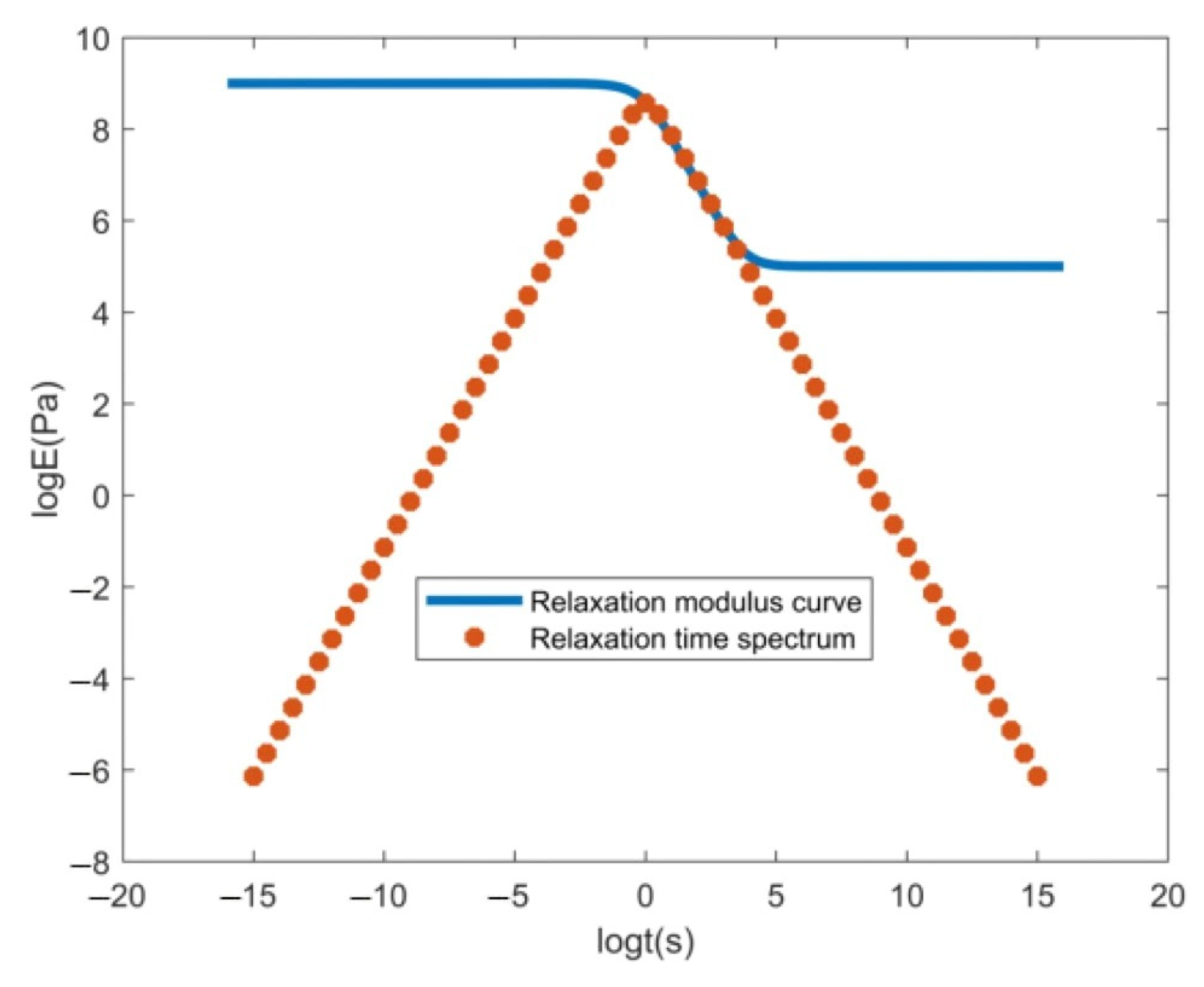
A simulated relaxation time spectrogram was drawn in the logarithmic coordinate system based on the quantitative relationship of Expressions (10)–(14). The following prerequisites were established: the relaxation time range considered in the logarithmic coordinate system spanned from −15 to 15; the relaxation time interval was set to 0.5; the number of spectral lines was set to 61; and
was set to
and
to
. The resulting graph is presented in
Figure 2.
Based on the findings from
Section 3, the relaxation spectral lines outside the relaxation time boundary can be discarded. It is imperative to evaluate whether the reduced relaxation spectrum effectively represents the unreduced relaxation spectrum. This analysis mainly focused on four distribution forms of the relaxation time spectra: slope, trapezoid, Lorentz, and Gaussian. The logarithmic time interval of the relaxation modulus function was set to [−16, 16]. The relaxation modulus function curve was generated by plotting a point at every 0.1 unit of logarithmic time. For each distribution form, the relaxation time spectra with 61 spectral lines and a time interval of 0.5 logarithmic units, and their corresponding relaxation modulus curves, are illustrated in
Figure 3,
Figure 4,
Figure 5 and
Figure 6.
The reduction method depends on specific circumstances and mainly considers two aspects as follows:
- (1)
The characteristic region of the stress relaxation curve exhibited by the viscoelastic material at a given temperature.
- (2)
The deviation between the relaxation modulus calculated by the reduced model and that generated by the original model.
Simplified calculations were conducted across several logarithmic time intervals, [−16, −14], [−12, −10], and [−8, −6], to explore the error of the relaxation modulus after reducing the relaxation spectrum. The following preparation steps were undertaken before conducting the calculations:
- (1)
Determination of the logarithmic testing time range: the three logarithmic time intervals mentioned above.
- (2)
Determination of the relaxation time limit: The two logarithmic units were extended outward from the leftmost side of the selected time range to serve as the lower bound of the relaxation time. Similarly, the time range was extended outward by four logarithmic units on the far right to serve as the upper bound for relaxation time.
The number of spectral lines was increased to 121 and 241 to comprehensively study the characteristic region suitable for applying the spectral line reduction method. The same logarithmic time interval was selected in different regions for calculation and comparison. The calculation results are summarized in
Table 1.
The results presented in
Table 1 indicate the following:
- (1)
With the exception of the data exhibiting a trapezoidal distribution in the logarithmic time interval of [−16, −14], an increase in the number of relaxation time spectral lines of all types within any distribution interval led to a higher sum of squared residuals of the relaxation modulus data resulting from the model reduction before and after.
- (2)
When using the “spectral line reduction method” to simplify the mechanical characterization model of viscoelastic materials, except for the slope-type, the sum of squared residuals increased for the other types of relaxation spectrum distributions as the logarithmic time interval shifted to the right.
- (3)
In summary, for all types of relaxation spectrum distributions, the sum of squared residuals across all logarithmic time intervals was less than 1 × 10⁻¹⁰. Therefore, the “spectral line reduction method” proposed in this paper is practical and feasible.
5. Research on Calculation of Indentation Rolling Resistance Based on Relaxation Model Parameters
The “spectral line reduction method” can be used to assess the viscoelastic relaxation modulus of the transmission belt, facilitating the substitution of the relaxation modulus into the formula for calculating indentation rolling resistance. This enables the determination of indentation rolling resistance under different operational conditions. An introduction to the theoretical basis for calculating indentation rolling resistance is presented in the subsequent section.
5.1. Theoretical Basis of Calculation of Indentation Rolling Resistance
The calculation of indentation rolling resistance, viewed from a temporal perspective, mainly addresses the operational resistance encountered in belt conveyors. As the conveyor belt moves on the rollers, it undergoes compression, leading to deformation. Subsequently, as the conveyor belt moves, the rollers gradually disengage from contact with the conveyor belt, resulting in a residual deformation that persists. This phenomenon of hysteresis creates indentation rolling resistance between the conveyor belt and the rollers. To conceptualize the scenario of contact between the conveyor belt and the roller, we established a model: the interface between the conveyor belt and the roller was likened to the surface of a viscoelastic material, whereas the roller was treated as a rigid cylinder. A schematic representation of the model established in this study is shown in
Figure 7.
In the illustration of the model,
refers to the thickness of the covering layer;
denotes the speed of the conveyor belt movement;
represents the initial contact point between the conveyor belt and the roller;
denotes the position where the conveyor belt and the roller disengaged;
represents the radius of the roller;
denotes the depth of indentation during stable motion; and
represents the depth of indentation at different positions. Previous findings indicate that, assuming that
is significantly smaller than
, after sequential integration and other numerical operations [
23], the following equations can be obtained:
In the above expressions, where represents the load, denotes the indentation rolling resistance, ,, and are viscoelastic parameters, , and . Viscoelastic parameters, , , , and are established constants.
The values of and can be determined by setting an initial value for and iteratively solving Equations (15) and (16). Subsequently, the indentation rolling resistance can be determined by substituting the values of and as well as other parameters into Equation (17).
5.2. Numerical Calculation of Indentation Rolling Resistance under Different Time Ranges
Different time ranges can denote the testing time range corresponding to the relaxation modulus and the relaxation time span of the relaxation time spectrum. These distinct relaxation time ranges also correspond to different characteristic regions of the material, such as glass state, glass transition zone, equilibrium state, and viscous flow state. In this section, the numerical characteristics of indentation rolling resistance under different time range conditions are explored using the “spectral line reduction method”. The parameters of the working conditions were an idler radius () = 0.08 m; a thickness of the conveyor belt cover layer of 0.008 m; and a vertical load of 2000 N/m. Simulation analysis was conducted by varying the magnitude of the speed.
For the Lorentz-type relaxation spectrum model, considering and , the number of spectral lines was 61. The calculation of indentation rolling resistance across different time ranges was conducted to determine the sensitivity of viscoelastic materials to stress over time. Consequently, four testing time intervals were selected in the logarithmic coordinate system: [−14, 6], [−14, −8], [−8, −2], and [−2, 4]. Using the “spectral line reduction method”, the relaxation time range in these intervals were determined as follows: [−16, 7], [−16, −4], [−10, 2], and [−4, 7]. Subsequently, the iterative equation solving method outlined in the previous section was used to determine the indentation rolling resistance. In the interval [−14, 6], the ratio of the sum of relaxation spectral line intensities to the total relaxation spectral intensity was 0.9999. Therefore, the relaxation spectrum within the interval adequately represents the relaxation spectrum of the Lorentz-type material. The calculated indentation rolling resistance within this interval can be considered as the actual indentation rolling resistance. The calculated indentation rolling resistance value in other intervals can be compared with this established actual indentation rolling resistance value.
The findings showed that the calculated indentation rolling resistance in the interval [−14, 6] aligns closely with the actual indentation rolling resistance (
Figure 8). Conversely, the calculated indentation rolling resistance values within the intervals [−14, −8] and [−2, 4] were smaller than the true values, with the values in the interval [−2, 4] exhibiting the smallest values. Notably, the calculated indentation rolling resistance values within the interval [−8, −2] were closest to the actual indentation rolling resistance values.
Similarly, and were set as the parameters for the Gaussian-type relaxation spectrum model, and the number of spectral lines was set to 61. Four testing time intervals were selected in the logarithmic coordinate system: [−10, 2], [−10, −6], [−6, −2], and [−2, 2]. The process of solving the indentation rolling resistance was similar to that used for the Lorentz-type. The indentation rolling resistance calculated on the interval [−10, 2] was considered as the actual value. The values obtained for the other intervals were compared with the set of actual indentation rolling resistance values.
The following numerical patterns were obtained by evaluating the results presented in
Figure 8 and
Figure 9:
- (1)
Within the interval [−14, −8], the Lorentz-type material exhibited a glassy state with low viscosity. When the roller rolled on the surface of the material, the strain lagged behind the stress briefly, resulting in a lower indentation rolling resistance than the actual value.
- (2)
As the Lorentz-type material transitioned from the [−8, −2] interval, it moved between the glassy and the elastic platform zone. The Gaussian-type material spanned the [−10, −6] and [−6, −2] intervals, showing significant viscosity. When the roller rolled on the surface of the material, the strain lagged behind the stress for a long time, resulting in significant indentation rolling resistance. During this phase, the indentation rolling resistance was close to the actual value.
- (3)
In the conventional state, the two materials were located in the elastic plateau region in the interval [−2, 4] and [−2, 2], and they exhibited low viscosity. Consequently, when the roller interacted with the surface of the material, the delay between the strain and stress was minimal, resulting in the lowest possible the indentation rolling resistance.
- (4)
The fluctuations in the calculated indentation rolling resistance across various regions of materials could be attributed to the different relaxation spectrum parameters obtained in distinct testing time intervals. This indicates the variation of E0 and other parameters in the 2N + 1 component Maxwell model across different testing time ranges. Therefore, this model is applicable within a specific testing time range rather than serving as a universally theoretical model.


