Abstract
This paper proposes a reinforcement learning method using a deep residual shrinkage network based on multi-reward priority experience playback for high-frequency and high-dimensional continuous vibration control. Firstly, we keep the underlying equipment unchanged and construct a vibration system simulator using FIR filters to ensure the complete fidelity of the physical model. Then, by interacting with the simulator using our proposed algorithm, we identify the optimal control strategy, which is directly applied to real-world scenarios in the form of a neural network. A multi-reward mechanism is proposed to assist the lightweight network to find a near-optimal control strategy, and a priority experience playback mechanism is used to prioritize the data to accelerate the convergence speed of the neural network and improve the data utilization efficiency. At the same time, the deep residual shrinkage network is introduced to realize adaptive denoising and lightweightness of the neural network. The experimental results indicate that under narrowband white-noise excitation ranging from 0 to 100 Hz, the DDPG algorithm achieved a vibration reduction effect of 12.728 dB, while our algorithm achieved a vibration reduction effect of 20.240 dB. Meanwhile, the network parameters were reduced by more than 7.5 times.
1. Introduction
When it comes to active vibration control, we face a high-dimensional, high-frequency, continuous, and complex dynamic problem. In order to cope with this challenge, a variety of traditional methods have been proposed. For example, PID controllers [1,2,3,4] are used to control complex objects, especially those with large time delays, rapid parameter changes, significant uncertainties, and severe nonlinearity. However, the PID controller has poor control quality in these cases, and a large number of parameters need to be designed in advance. Another common method employs the LQR controller [5,6,7], which uses a quadratic performance index. However, in practical applications, not every scenario is suitable for such an indicator, and it can only be applied to systems that can be represented by state-space equations. Another method involves the FxLMS controller [8,9,10], which not only needs to construct the reference signal, but also needs to identify the auxiliary path. However, studies have shown that although these traditional methods can play a role in control, they all require a lot of design work and manual intervention.
In recent years, the use of reinforcement learning (RL) technology to improve the efficiency of vibration controller designs has become a method of great concern. This method uses the reinforcement learning algorithm to automatically obtain the parameters of the controller, which brings new possibilities for vibration control. Compared with traditional methods, the reinforcement learning method is a data-driven approach, which does not require physical information on vibration control, such as the mass matrix, damping matrix, and stiffness matrix, thus reducing the required engineering and design investment. In fact, the use of reinforcement learning methods to construct agents to learn vibration control in complex environments has achieved remarkable results [11,12,13,14,15]. This method has been applied in many fields, such as for suspension vibration control [16,17], manipulator vibration control [18,19,20], magnetorheological damper vibration control [21,22], and other vibration control applications [23,24,25], and has made remarkable progress.
In the field of suspension vibration control [16,17], Li et al. [16] integrated model-free learning with model-based safety supervision. They used the underlying system dynamics and security-related constraints, used recursive feasibility techniques to construct security sets, and integrated them into the detection system constraints of reinforcement learning. This secure reinforcement learning framework was applied to the active suspension control system. Their experiments show that this secure reinforcement learning system can learn the control strategy safely and has better performance than the standard controller. Zhao et al. [17] discussed the set value tracking problem for the suspension system of a medium-speed maglev train, aiming at maintaining a fixed distance between the train and the track. They describe the set point tracking problem as a continuous-state and continuous-action Markov decision process under unknown transition probabilities, and obtain the state feedback controller from the sampled data of the suspension system through a Deterministic Policy Gradient and neural network approximation reinforcement learning algorithm. Their simulation results demonstrate the high performance of this model-free method, especially given that the response speed of their controller is 50 times faster than that of PID and no additional modeling work is required.
In the field of robotic arm control [18,19,20], Ding et al. [18] proposed an innovative human–computer interaction system and applied it to the cooperative operation control task of a robotic arm. Their human–computer interaction system includes an impedance model controller and a manipulator controller. The model-based reinforcement learning method is applied to the impedance mode for operator adaptation. The newly designed adaptive manipulator controller realizes a speed-free filter. Their simulation results verify the effectiveness of the human–computer interaction system based on the real manipulator parameters. On the other hand, Adel et al. [19] proposed a learning framework for robot manipulators based on nonlinear model predictive control, which aims to solve the motion planning problem of robot manipulators in the presence of obstacles. The cost function, system constraints, and manipulator model were parameterized by using the value function of the reinforcement learning framework and the myopic value of the action-value function. The controller was applied to the robot manipulator of a 6-DOF model. Their numerical simulation results show that this controller can effectively control the attitude of the end effector, avoid the collision between the manipulator and the obstacle, and improve the efficiency of the control loop by 21%. Additionally, Vighnesh et al. [20] designed a two-wheeled inverted pendulum mobile manipulator for retail shelf inspections. In comparison to PID control, in simulation tests, the controller based on reinforcement learning exhibited stronger robustness against variations in initial conditions, changes in inertia parameters, and disturbances applied to the robot.
In the field of magnetorheological damper vibration control [21,22], Park et al. [21] proposed a reinforcement learning method for magnetorheological elastomer vibration control based on Q-learning. Their research shows that it is feasible to use a model-free reinforcement learning model to realize an adaptive controller based on the application of highly nonlinear magnetorheological elastomers. When compared with a model without the controller, this method suppressed the vibration level by up to 57%. In addition, Yuan et al. [22] proposed a magnetorheological damping semi-active control strategy based on a reinforcement learning Q-learning algorithm. Their simulation results show that this method is simpler, easier to implement, and more robust. They used the reinforcement learning semi-active control strategy to study the vibration reduction of a two-story frame structure. The results show that the strategy is superior to the simple bang–bang control method.
At present, some progress has been made in the combination of reinforcement learning and finite-impulse response filters. Feng et al. [26] successfully solved the multi-input/multi-output actual vibration control problem in a frequency range by using RL and FIR filters, which marks the first time that reinforcement learning has been used to solve high-dimensional high-frequency vibration control problems. In order to meet the lightweight requirements of the underlying equipment, they designed the simplest fully connected neural network. However, this method may face the challenge of overfitting or underfitting when solving more complex and variable dynamic problems. In order to solve this problem, we try to find a way to both maintain lightweightness and solve complex problems.
In the field of deep learning, the way to achieve lightweightness is to reduce resource consumption and model complexity. In this regard, some achievements have been made [27,28,29,30]. Among the research on lightweightness, He et al. [27] proposed a residual network framework to reduce the burden of network training. They explicitly redefined each layer as the input of the reference layer and learned the residual function instead of learning an unknown function. Through comprehensive experimental data, they clarified that their residual network is easier to optimize, and that increasing the network depth can achieve higher accuracy. This method improved the results in the COCO target detection dataset by 28%, and won the first place in the COCO target detection and image segmentation tasks. On the other hand, Howard et al. [28] proposed an efficient model called MobileNets, which uses deep separable convolution to construct a lightweight deep neural network. Through extensive resource and accuracy experiments, MobileNets showed strong performance compared with other popular ImageNet classification models. They also demonstrate the effectiveness of this method in object detection, fine-grained classification, face attributes, and large-scale geolocation. Zhang et al. [29] proposed a computationally efficient CNN architecture called ShuffleNet. This method uses two new operations, point group convolution, and channel rearrangement, which greatly reduces the computational cost while maintaining accuracy. Their experiments on ImageNet classification and MS COCO target detection show that ShuffleNet is superior to other structures. On ARM-based mobile devices, the speedup of ShuffleNet is about 13 times higher than that of AlexNet, and it maintains considerable accuracy. In addition, Zhao et al. [30] proposed a deep residual shrinkage network to improve the feature learning ability of high-noise vibration signals. They inserted the adaptive soft threshold as a nonlinear transformation layer into the deep architecture to eliminate unimportant features. The effectiveness of their developed method was verified through various types of noise experiments.
At present, reinforcement learning forms a very mature system. It is mainly divided into two categories: value-based learning and probability-based learning, and has algorithms that combine these two methods. Probability-based reinforcement learning is one of the most direct methods and makes decisions by directly outputting the probability of the next possible action. In this method, each action has the opportunity to be selected, but the size of these opportunities is different. For example, the Policy Gradients approach [31] is a probability-based approach. In contrast, the value-based approach involves outputting the value of all actions and selecting the action with the highest value in the decision-making process. For example, algorithms such as Q-learning [32] are value-based methods. Combining the advantages of these two methods, some more optimized algorithms have been derived, such as Actor–Critic [33]. In this structure, the Actor makes an action based on probability, while the Critic assesses the value of the action. This combination optimizes the original Policy Gradients approach and accelerates the learning process. At present, the AC method has many extensions, including the Deep Deterministic Policy Gradient (DDPG) [34], Soft Actor–Critic (SAC) [35], and Twin Delayed Deep Deterministic Policy Gradient (TD3) [36] techniques.
Regarding the Actor–Critic method of reinforcement learning, Lillicrap et al. [34] proposed an Actor–Critic model-free algorithm based on Deterministic Policy Gradients, which can operate in a continuous-action space. They successfully solved the challenges of more than 20 simulated physical tasks by using the same learning algorithm, network architecture, and hyperparameters. Haarnoja et al. [35] described the Soft Actor–Critic approach, which is an offline strategy Actor–Critic algorithm based on a reinforcement learning framework. Its goal is to maximize both the expected return and entropy. This method is superior to the previous online strategy and offline strategy methods in terms of the sample utilization efficiency and progressive performance. In addition, Fujimoto et al. [36] found that in value-based reinforcement learning methods, known function approximation errors may lead to overestimation and suboptimal strategies for value estimation. Based on this, they propose a new mechanism called Twin Delayed Deep Deterministic Policy Gradient to mitigate the overestimation issues of Actor–Critic algorithms. They suggest constraining overestimation by taking the minimum of a pair of critics based on the foundation of double Q-learning. When evaluating their approach, it consistently outperformed current state-of-the-art methods across various testing environments.
However, due to the large number of parameters required in stacking neural networks to solve complex problems, previous algorithms have limitations such as algorithmic simplicity or a larger parameter count, impacting the timely control of controllers. To address this issue, this paper proposes vibration control with reinforcement learning based on a multi-reward lightweight network. Specifically, it is a deep residual shrinkage lightweight method based on deep reinforcement learning with multi-reward prioritized experience replay (DRSL-MPER). We introduce a multi-reward mechanism to assist the TD3 algorithm in finding control policies close to optimal. At the same time, we also introduce a priority experience playback mechanism to assign priority to the data, thereby accelerating the convergence speed of the neural network and improving the data utilization efficiency. In addition, we also introduce a deep residual shrinkage network to achieve adaptive denoising and lightweightness of the neural network. The algorithm proposed in this paper has two significant and practical advantages. Firstly, it employs a lightweight network, which not only enhances the computational efficiency and reduces the energy consumption but also facilitates deployment and maintenance in real-world scenarios, while supporting rapid iterative updates of the system. Secondly, the algorithm demonstrates excellent control performance and good generalization capabilities, which can significantly improve the performance and lifespan of equipment, enhance the reliability and safety of the system, and increase its adaptability and flexibility.
The rest of this paper is organized as follows: Firstly, the vibration control problem is described. Secondly, our lightweight method of multi-reward priority experience playback based on deep reinforcement learning is proposed. Then, the vibration controller designed using this method is verified through experiments. Finally, we draw our conclusions.
2. Problem Formulation
2.1. Dynamic Model
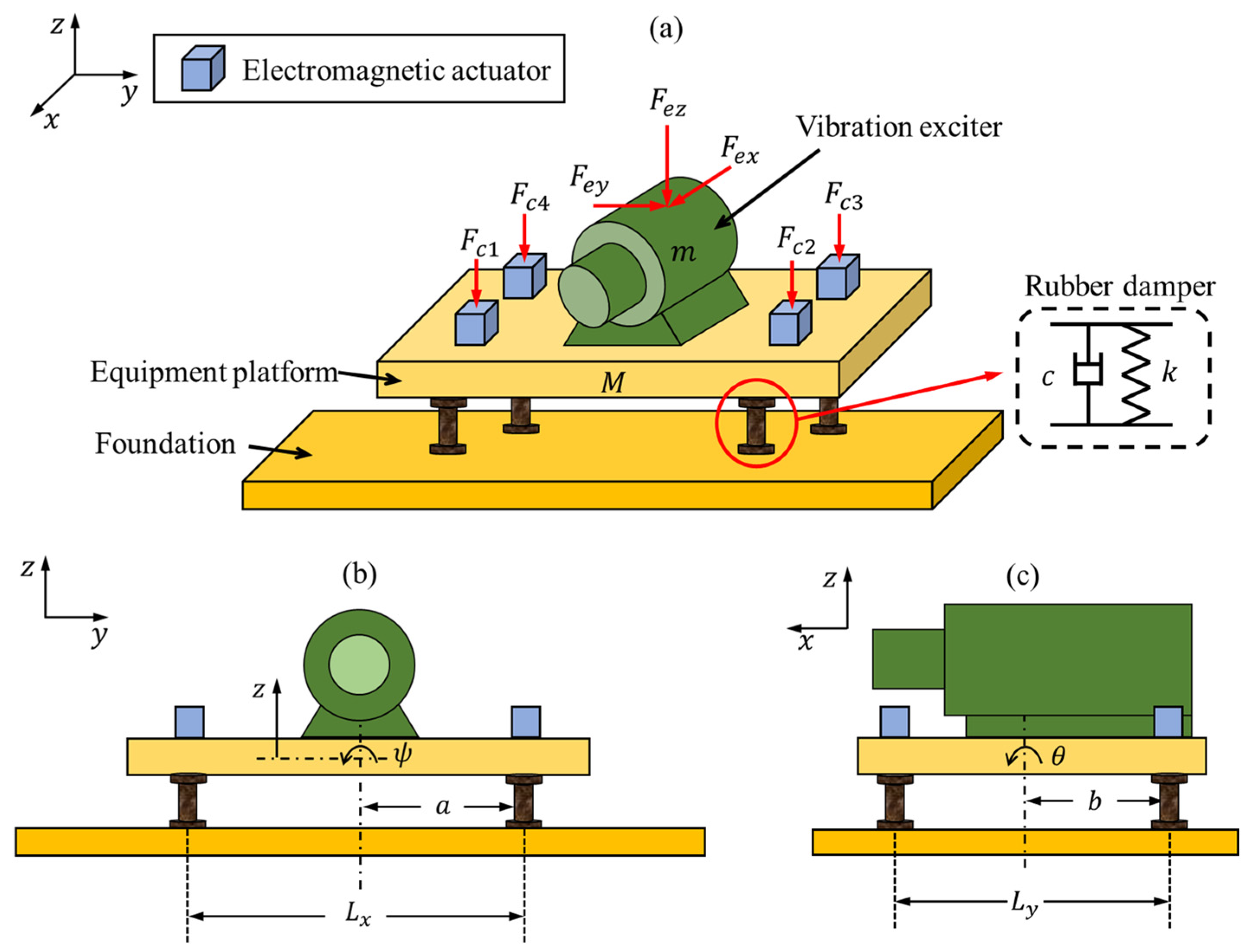
Figure 1 shows the dynamic model of the high-dimensional high-frequency vibration control system considered in this paper. The vibration exciter is installed on the equipment platform , which is supported on the foundation by four rubber dampers. The rubber dampers can be regarded as a spring damping system composed of linear spring and linear damping . Four electromagnetic actuators are mounted on the equipment platform, which generate counteracting control forces to reduce the vibration of the equipment platform caused by the vibration exciter. The rotation angles of the equipment platform around its horizontal inertia principal axes paralleling to the -axis and -axis are and . The vibration exciter generates excitation forces in three directions, denoted as . However, since the actuators can only generate control forces in the -direction (), only the translational motion along the -axis and the rotational motion around the horizontal axis are considered. Thus, there are three generalized coordinates in the dynamic model: .
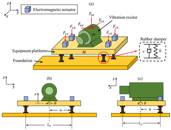
Figure 1.
Schematic of the vibration control system: (a) axonometric view; (b) front view; (c) right view.
Using the Lagrange equation, the dynamic equations of the vibration control system can be described as follows:
where and represent the moment of inertia of the system with respect to the -axis and -axis, = 100 kg, = 913 kg, = 1.6 m, = 1.2 m, = 0.8 m, = 0.6 m, = 76 kg*m2, = 58 kg*m2, = 600,000 N/m, and = 100 Ns/m.
The equipment platform generates vibrations in the z-direction subjected to the excitation force . It is evident from Equations (1)–(3) that by adjusting the value of the control forces , the vibrations of the equipment platform can be reduced, achieving active vibration control. In this paper, the vibration exciter is supposed to generate random multi-frequency excitations, making this vibration system a typical high-dimensional high-frequency vibration control problem.
2.2. Active Control Implementation
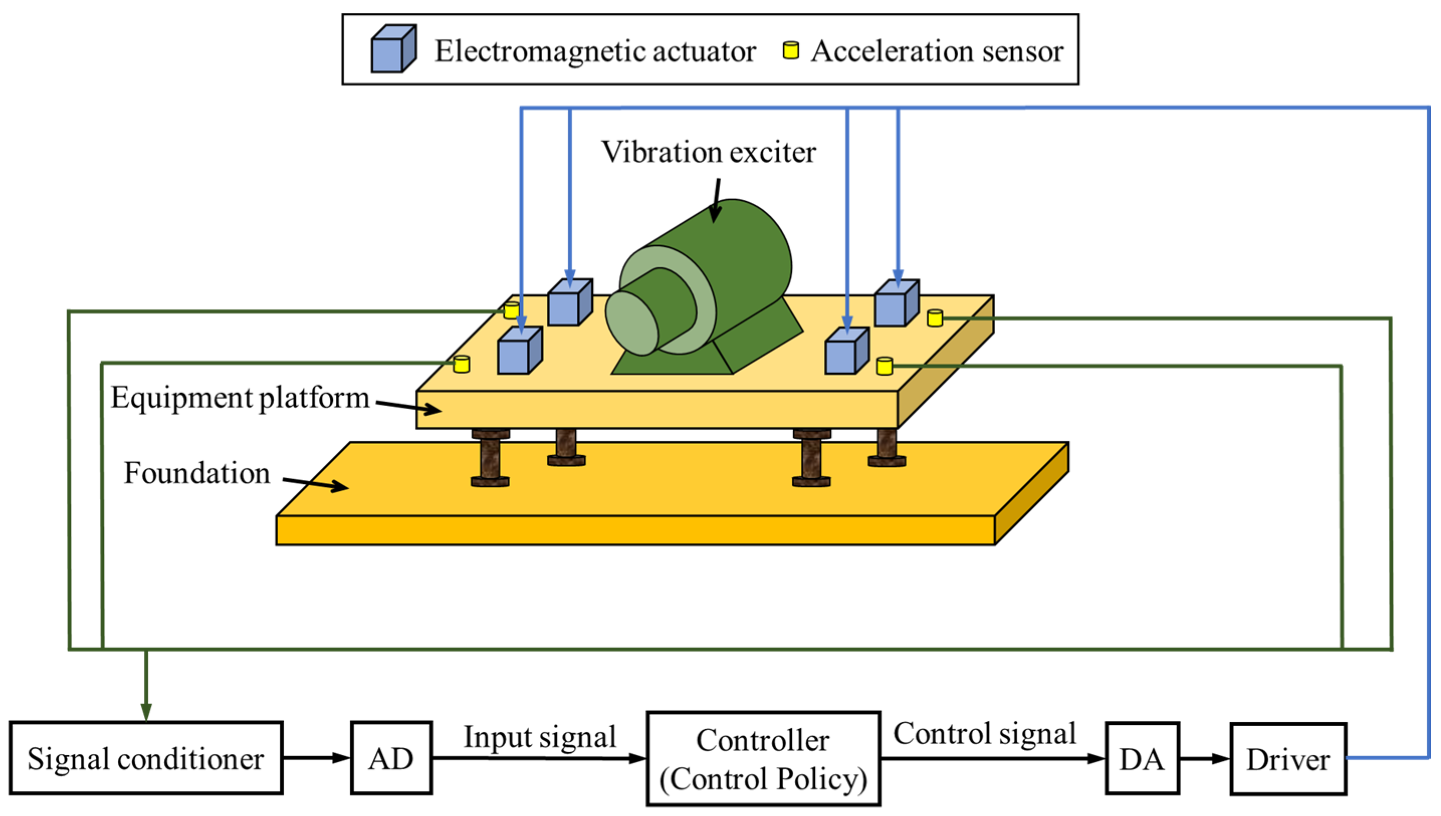
In active vibration control, the control algorithm needs to calculate the control signal based on the system’s response. This section presents the implementation of the high-dimensional high-frequency vibration control problem, as shown in Figure 2. An acceleration sensor is installed near each of the four electromagnetic actuators to collect the acceleration signals at the respective positions. The four control signals are computed in real time by the controller running a trained reinforcement learning neural network, based on signals from the four acceleration sensors located near the actuators. The signal conditioner is used to filter and amplify the signals from the four acceleration sensors, which are then converted into digital signals via an AD module and fed into the controller for processing. The control signals are amplified by a driver into control current signals after being processed via a DA module to drive the actuators. The electromagnetic actuator consists of a permanent magnet armature and a coil, with the permanent magnet armature positioned in the middle of the coil. When current flows through the coil, the permanent magnet armature moves up and down under the influence of the coil’s magnetic field, generating actuating force. The driver is a power amplifier that amplifies the control signal calculated by the controller into current to drive the electromagnetic actuator to operate.

Figure 2.
The active vibration control process of the vibration control system.
Since the vibration control system is often applied in complex vibration environments, where theoretical models cannot accurately describe the input–output response of the system, real experimental data are used for the research in this paper. In the following sections, the vibration control system is modeled as a simulator constructed from these experimental data. Based on the simulator, a neural network vibration controller is designed using reinforcement learning methods to solve the high-dimensional high-frequency vibration control problem.
3. Method
3.1. Vibration System Simulator
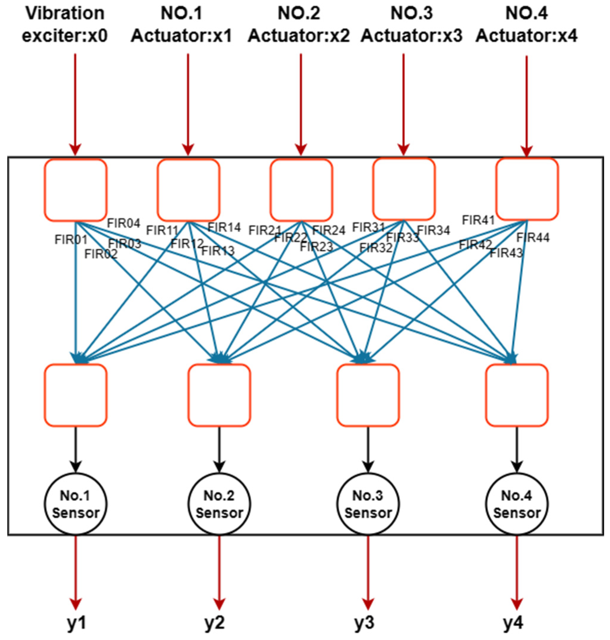
Figure 3 shows the vibration control simulator built using the finite-impulse response (FIR) filter. This simulator is used to describe the real vibration control system shown in Figure 1, involving five inputs and four outputs. Among them, the five inputs represent the force of the exciter and four electromagnetic actuators; the four outputs correspond to four acceleration signals. Before establishing the simulator, narrowband Gaussian white-noise force signals ranging from 0 to 100 Hz are separately inputted into the exciter and the four actuators, and experimental data from the four acceleration sensors are pre-collected. Subsequently, the input force signals and the collected acceleration data are used for the identification process of the FIR filters. These filters make up the simulator, which is capable of simulating the responses of the four acceleration sensors in the real vibration system by applying specified force signals to the exciter and electromagnetic actuator.
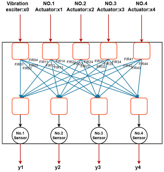
Figure 3.
Description of the vibration system simulator. The FIR filter-identified signal is shown in blue, while the input–output vibration signal is shown in red.
3.1.1. FIR Filter
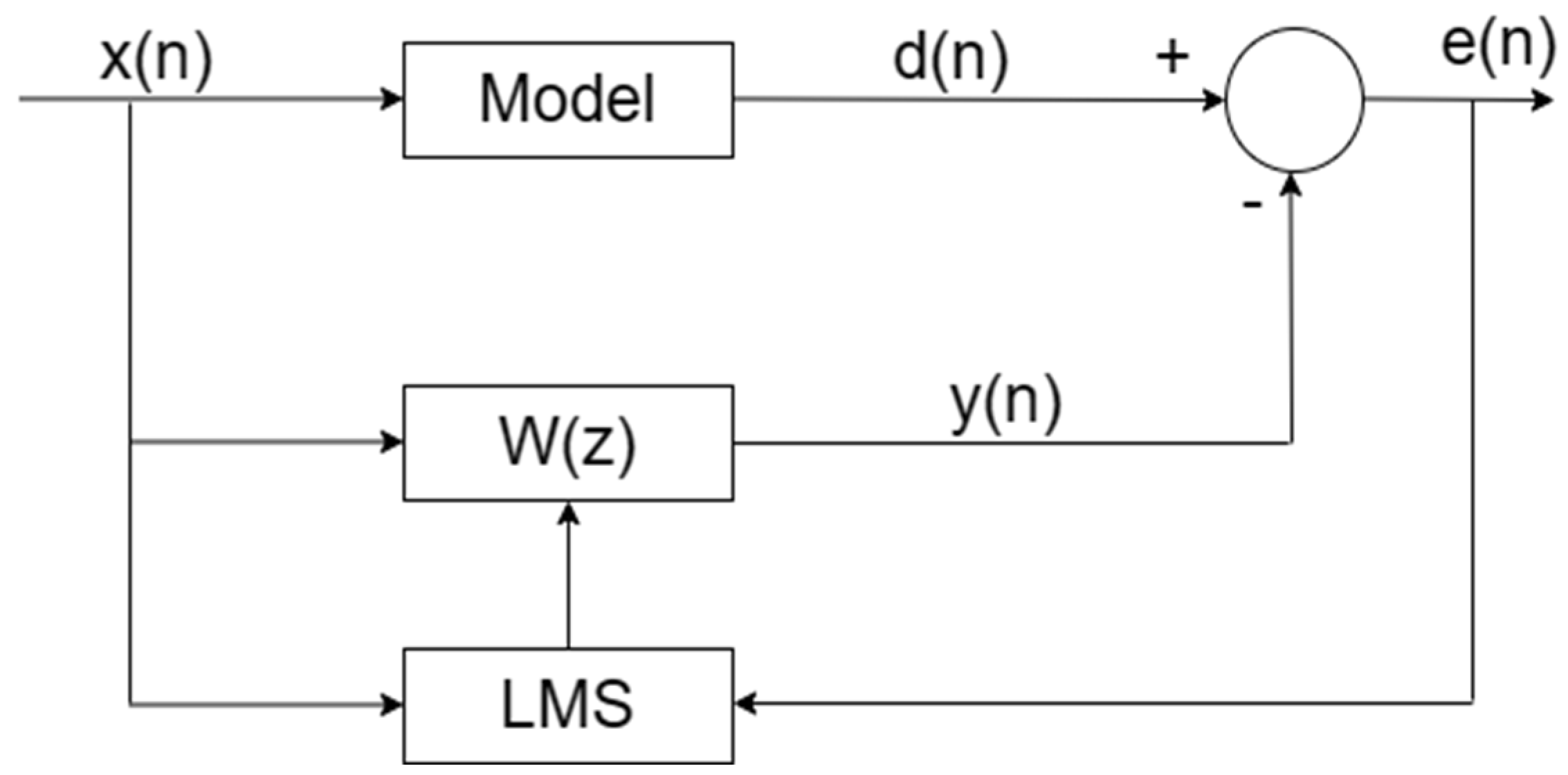
Adaptive FIR filters are used to construct the simulator. As shown in Figure 4, in order to realize the FIR filter, we need to obtain the input signal and the desired input and output signals , and as vectors:
where is the length of the filter. The input signal of a given filter is known, and the output signal of the filter is expressed as follows:
where n indicates the serial number of the discrete-time data, and is the vector of the filter value.

Figure 4.
Schematic diagram of an FIR filter.
The output signal is the estimation of the desired signal . The error between the output signal and the desired signal is defined as follows:
By using the least-mean-square (LMS) algorithm [37], we estimate the filter weight to minimize the error :
where is the step size.
If the appropriate input signal and the desired output signal are given, it is easy to estimate the filter weight . In this paper, both the input signal and the expected output signal are experimental data.
3.1.2. Using FIR Filters to the Build Simulator
The simulator can be viewed as a five-input/four-output filter. The input signals are denoted as , , , and , where represents the force signal of the exciter, and , , , and represent the force signals of the four electromagnetic actuators. The required output signals are recorded as , , , and , which represent the acceleration signals, respectively. is the estimated value of the expected output (, j = 1, 2, 3, 4).
Obviously, there are 5 × 4 = 20 channels between the input and output, each of which can be represented by an FIR filter. We can suppose that represents a filter between and , where i = 0, 1, 2, 3, 4 and j = 1, 2, 3, 4.
Note that is the open-loop response under , , , and excitation. Therefore, the estimation of can be expressed as follows:
where is the estimated value of , and is the filter weight of the filter . It can be found that is the superposition of the outputs of five FIR filters. Similarly, the estimated values of , , and are expressed as follows:
Formulas (10)–(12) can be written as a reduced version of Formula (13), which is the simulator of the vibration system.
The simulator consists of 20 single-input/single-output filters. The matrix contains the weights of 20 filters, where is the weight vector of the filter : i = 0, 1, 2, 3, 4 and j = 1, 2, 3, 4.
3.2. Algorithm Framework
We consider a standard reinforcement learning setting consisting of an agent interacting with a discrete-time step-size environment . At each time step , the agent can receive the observed value , take an action , and receive a scalar reward . The behavior of the agent is defined according to the strategy , which maps the state to the probability distribution of the action :. The environment may also be random. We model it as a state-space , action-space , initial-state distribution , transition dynamics reward function . The reward is defined as the sum of future reward discounts:. The discount factor is ϵ [0,1]. The payoff depends on the chosen behavior, and therefore depends on the strategy , and may be random. The goal of reinforcement learning is to learn a strategy that maximizes the expected revenue of the initial distribution: . When = i, we use the minimum value of the output of the two critic networks, i.e., the output of and critic networks.
Many of the methods in reinforcement learning utilize the recursive relationship of the Bellman equation:
If the target policy is deterministic, we can describe it as a function , thus avoiding internal expectations.
Expectations depend only on the environment. This means that the transfer generated by different random behavior strategies can be used to learn the offline strategy. We consider a function approximator with as a parameter and optimize it by minimizing the loss:
Here, is the environmental reward, is the discount factor, and is the index of the next state.
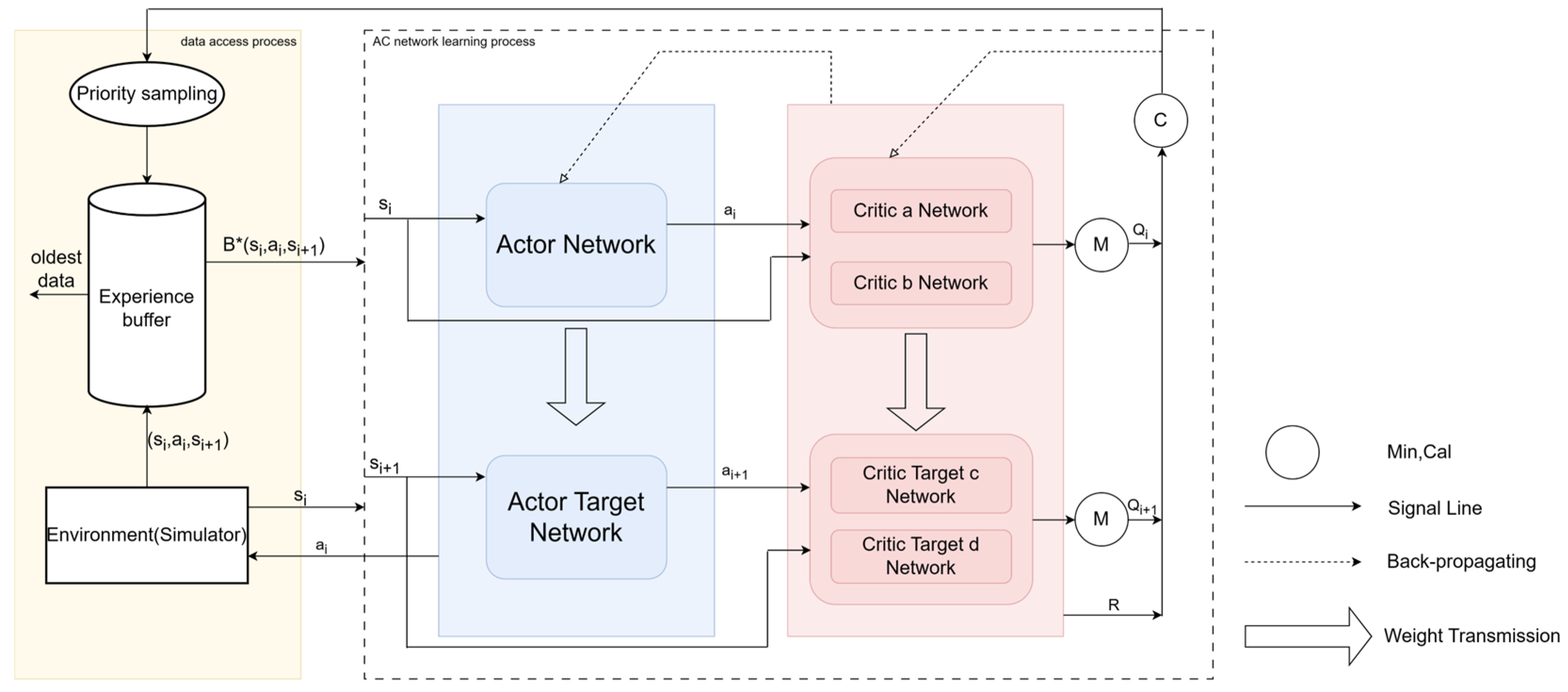
As shown in Figure 5, the algorithm used in this paper is mainly divided into two parts: the yellow part represents the environment (simulator) and experience playback, and the virtual part is the Actor–Critic (AC) network. Specifically, first, the environment interacts with the AC network and stores multiple data into the experience pool. Here, denotes the state at time , denotes the action at time , and denotes the state at time . Each data point in the experience pool is given an initial priority. When the data reach a certain amount, priority data sampling is performed for the data in the experience pool. is passed to the Actor network, and the Actor network is passed to the Critic a network and the Critic b network together with , based on ‘s . At the same time, is transmitted to the Actor Target network, and the obtained by the Actor Target network based on is transmitted to the Critic Target c network and the Critic Target d network together with . The task of the Critic networks is to score the actions obtained from the Actor network. Here, we use four Critic networks, where the Critic a network and the Critic b network take the minimum value, and the Critic Target c network and the Critic Target d network also take the minimum value. Finally, the error is calculated using the Formulas (20) and (21). The dotted arrow represents the feedback neural network, and the Actor network and Critic network are updated in this way. The Actor Target network and Critic Target network adjust the neural network parameters through weight transfer. The final error is calculated using the priority formula and then used to update the priority of the data in the experience pool. When the amount of experience pool data is large enough, older data can be removed to free up space.
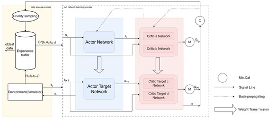
Figure 5.
Algorithm framework. Specifically, the algorithm is mainly divided into two parts: the yellow part represents the environment (simulator) and experience replaying, and the dotted line part represents the AC network.
In terms of updating the parameters, the critic network parameter update is as follows:
The Actor network updates the strategy according to the feedback of the critic network, that is, the gradient of the Q-value function:
where represents the output action of the Actor network to the state .
In addition, the Actor Target network and Target network update is as follows:
where i is the index of the Critic Target network and is the hyperparameter representing the weight of the update.
3.3. Actor–Critic (AC) Network
In this section, we focus on the AC network, where the Actor and Critic structures are the same, so we only need to explain one network structure. In order to make the network lighter and have a stronger generalization ability, we initially considered the application of convolution. However, in general, convolution requires multi-layer stacking, and too many neural network layers can easily lead to performance degradation, which may lead to gradient disappearance or gradient explosion. In order to solve this challenge, we considered and adopted the ResNet method [27]. Since we are dealing with vibration control problems, we further considered the variant deep residual shrinkage network (DRSN) [30] using ResNets.
3.3.1. Classic ResNet Architecture
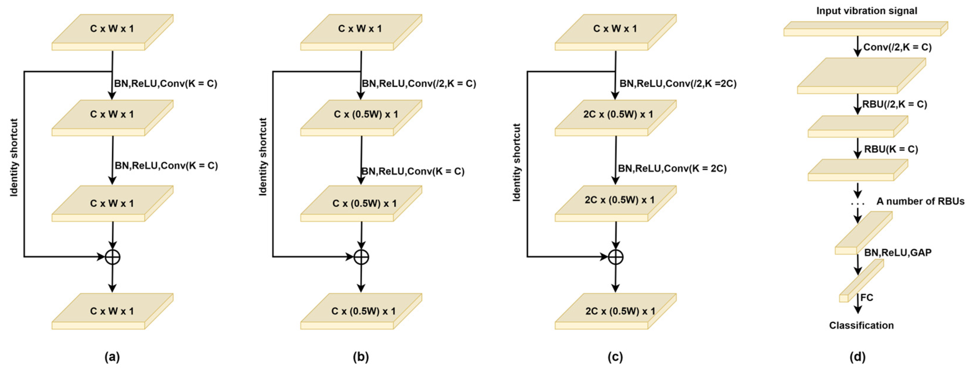
The ResNet approach an emerging deep learning method that has attracted much attention in recent years [27]. Remaining building units (RBUs) are the basic components. As shown in Figure 6a, an RBU consists of two BNs, two ReLUs, two convolutional layers, and a unit shortcut. The identity shortcut is the part that makes ResNets superior to convnets in general. In general, in convolutional neural networks, the cross-entropy error gradient is propagated backward layer by layer. Using the identity shortcut, the gradient can effectively flow to the earlier layer near the input layer, so that the parameters can be updated more effectively. Figure 6b,c shows the RBUs that produce output eigenmaps of different sizes. The aim of reducing the width of the output feature map is to reduce the amount of calculation for the next layer, and the aim of increasing the number of channels of the output feature map is to facilitate the integration of different features into discriminant features. Figure 6d shows the overall architecture of a ResNet, which consists of an input layer, a convolution layer, multiple RBUs, a BN, a ReLU, a GAP, and an output full-connection (FC) layer.
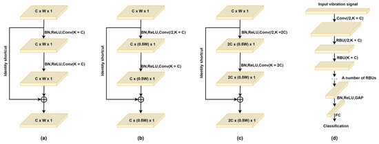
Figure 6.
Three kinds of remaining building units (RBUs), including (a) an RBU in which the output feature map is the same size as the input feature map; (b) an RBU with a stride of 2, in which the width of the output feature map is reduced to half of that of the input feature map; and (c) an RBU with a stride of 2 and a doubled number of convolutional kernels, in which the number of channels of the output feature map is doubled. (d) The overall architecture of a ResNet. In this figure, “/2” means to move the convolutional kernel with a stride of 2 to reduce the width of the output feature map; C, W, and 1 are the indicators of the number of channels, width, and height of the feature map, respectively; K is the number of convolutional kernels in the convolutional layer.
3.3.2. The Basic Architecture Design of DRSNs
In this section, the motivation for developing DRSNs is introduced, and the architecture of two developed DRSNs is described in detail, including a deep residual shrinkage network with channel-shared thresholds (DRSN-CS) and a deep residual shrinkage network with channel-wise thresholds (DRSN-CW).
- (1)
- Theoretical background
In the past 20 years, soft threshold segmentation has often been used as a key step in many signal denoising methods [37,38]. The advantage of this method is that it transforms the original signal into a domain where the number of near-zeros is not important, and then applies the soft threshold to convert the near-zero feature to zero. In order to ensure the good performance of signal denoising, a key task of the wavelet threshold method is to design a filter to transform useful information into very positive or negative features, and transform noise information into near-zero features. However, designing such filters requires a lot of signal processing expertise and has always been a challenging problem. Deep learning provides a new way to solve this problem. Deep learning is not designed by experts, but uses the gradient descent algorithm to automatically learn the filter. The formula for the soft threshold can be expressed as follows:
Within this formula is the input feature, the output feature, and the threshold, that is, the positive parameter. The soft threshold method does not set the negative features in the ReLU activation function to zero, but sets the features close to zero to zero, thereby retaining useful negative features.
It can be seen that the derivative of the output to the input is either 1 or 0, which can effectively prevent gradient disappearance and explosion problems. The derivative can be expressed as follows:
In a classical signal denoising algorithm, it is usually difficult to set an appropriate value for the threshold. In addition, the optimal value varies from case to case. To solve this problem, the threshold used in the developed DRSNs is automatically determined in the deep architecture, avoiding the trouble of manual operation. In the following chapters, the method of determining the threshold in the developed DRSNs will be introduced.
- (2)
- Developed DRSN-CS framework
The developed DRSN-CS is a variant of the ResNet, which uses soft thresholds to remove noise-related features. The soft threshold is inserted into the building unit as a nonlinear transformation layer. In addition, the value of the threshold can be learned in the building unit, as described below.
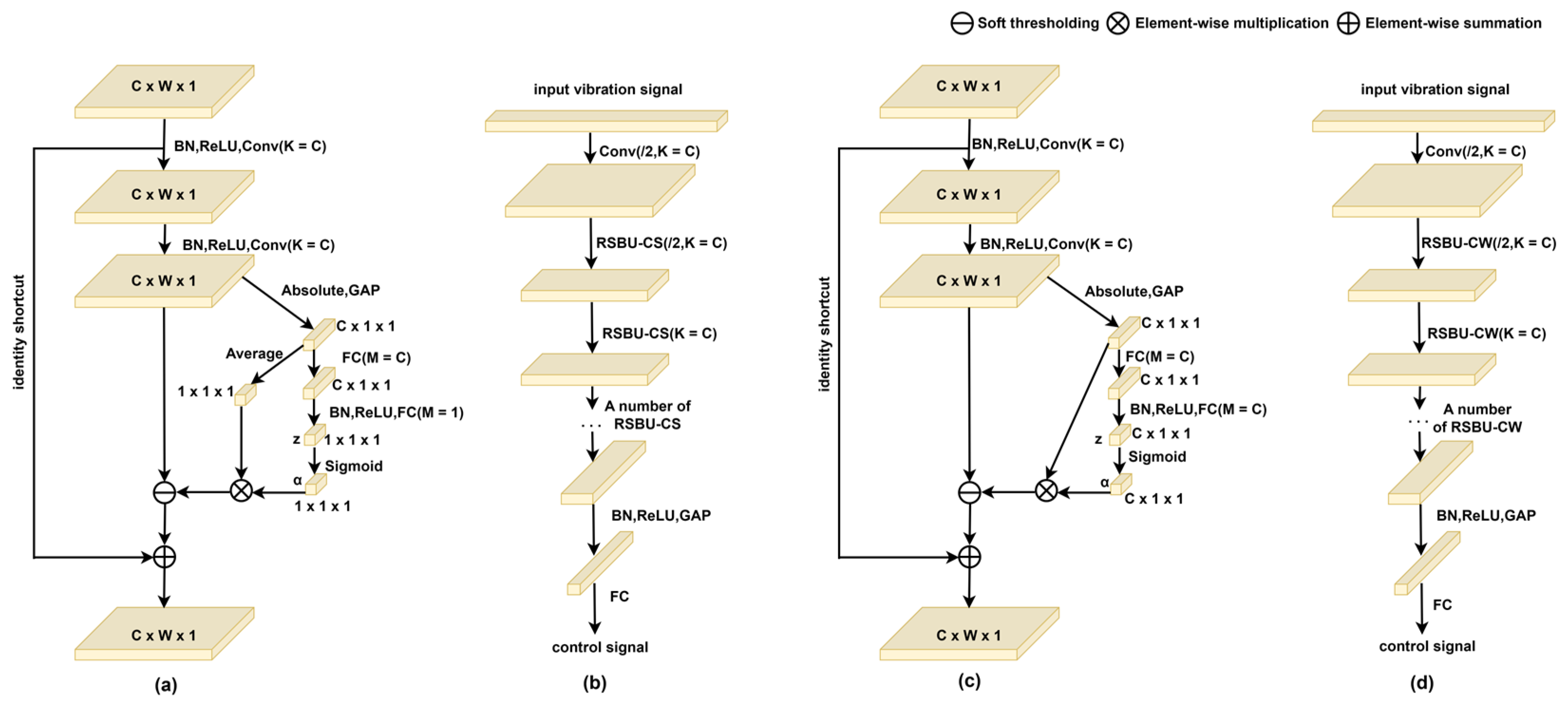
As shown in Figure 7a, unlike the RBU in Figure 6a, RSBU-CS has a dedicated module for soft threshold estimation. In this special module, Global Average Pooling (GAP) is performed on the absolute values of the feature map to obtain a one-dimensional vector. Then, the one-dimensional vector is propagated into a two-layer FC network to obtain a scaling parameter, similar to [39].
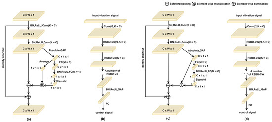
Figure 7.
(a) A residual shrinkage building unit with channel-shared thresholds (RSBU-CS). (b) DRSN-CS overall architecture. (c) A residual shrinkage building unit with channel-shared thresholds (RSBU-CW). (d) DRSN-CW overall architecture, where K is the number of convolution kernels in the convolutional layer; m is the number of neurons in the FC network; and the C, W, and 1 in C × W× 1 represent the number of channels, width, and height of the feature map, respectively. When determining the threshold, the index of the feature map to be used is .
The sigmoid function is applied at the end of the two-layer FC network so that the scaling parameters are scaled to the range of (0, 1), which can be expressed as follows:
From this equation, we can find the output of the two-layer FC network in the RSBU-CS, and the delay parameter is the corresponding scaling parameter. After that, the scaling parameter delay is multiplied by the average value of the score to obtain the threshold. The reason for this arrangement is that the threshold of the soft threshold should not only be positive, but also not too large. If the threshold is greater than the maximum absolute value of the feature map, the output of the soft threshold is zero. In summary, the thresholds used in the RSBU-CS are expressed as follows:
Here, is the threshold, and i, j, and c are the width, height, and channel index of the feature map, respectively. The threshold can be kept within a reasonable range so that the output of the soft threshold will not be all zeroes. The two-step RSBU-CS with a doubled number of channels can be constructed similar to the RBUs in Figure 6b,c.
The brief architecture of the developed DRSN-CS is shown in Figure 7b, which is similar to the classic ResNet in Figure 6d. The only difference is that the RSBU-CS is used as a building block instead of RBUs. Multiple RSBU-CSs are stacked in the DRSN-CS to gradually reduce noise-related features. Another advantage of the DRSN-CS is that the thresholds are automatically learned in the deep architecture, rather than being manually set by experts. Therefore, professional signal processing knowledge is not required to implement the developed DRSN-CS.
- (3)
- Developed DRSN-CW framework
The developed DRSN-CW is another variant of a ResNet. Unlike the DRSN-CS, it applies a separate threshold to each channel of the feature map, which will be introduced below. Figure 7c shows the RSBU-CW. Through absolute operation and the GAP layer, the upper and lower lines of the feature map are reduced to one-dimensional vectors, and they are propagated to the two-layer FC network.
Here, zc is the feature at the cth neuron, and is the cth scaling parameter. After that, the threshold can be calculated:
where i, j, and denote the width, height, and channel index of the feature map x, respectively. Similar to the DRSN-CS, the threshold can be positive and maintained within a reasonable range to prevent the output feature from being all zeros.
The overall architecture of the developed DRSN-CW is shown in Figure 7d. By superimposing multiple RSBU-CWs, through various nonlinear transformations, the soft threshold is used as the shrinkage function to learn the discriminant features and eliminate the noise-related information.
- (4)
- Detailed Network Architecture of the Actor
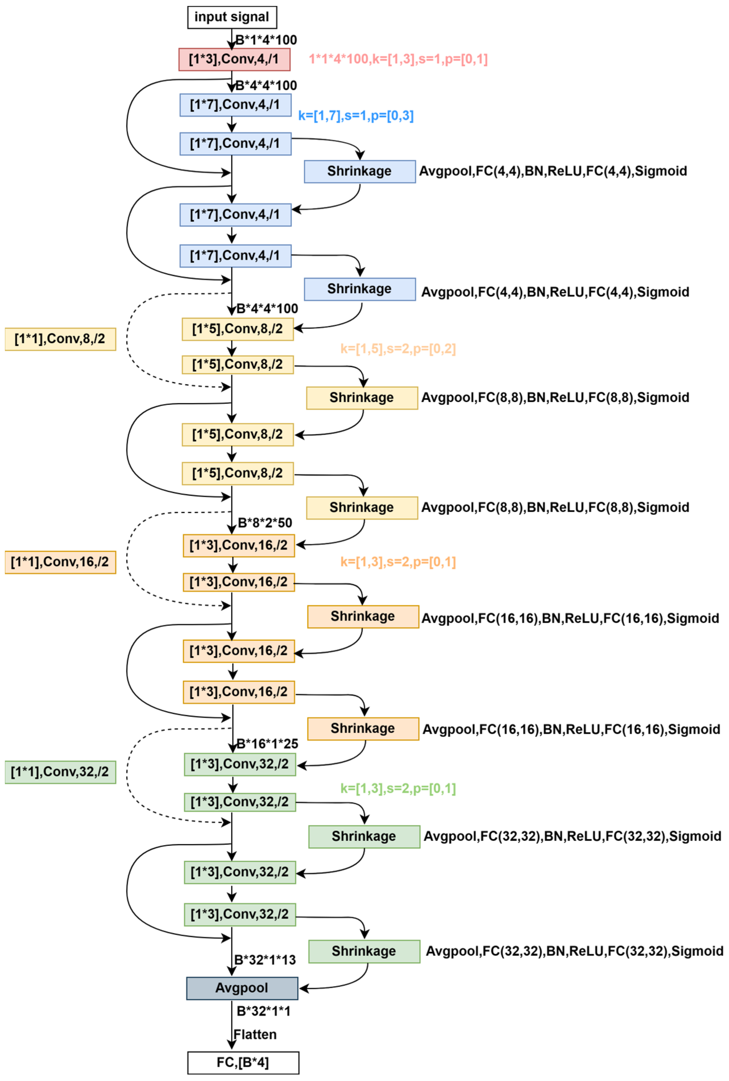
In Figure 8, there are dashed- and solid-line skips. When the input and output dimensions are the same (solid-line skips), residual learning is directly applied, i.e., , where represents the output result of the construction unit. In cases where the dimensions increase (dashed-line skips), matching dimensions occur (achieved by 1 × 1 convolution) with a stride of 2. Finally, through Avgpooling and flattening, we obtain [B, 32], which, via FC, leads to [B, 4] dimensions, representing the action signals from four sensors. The structure of the Critic’s four networks resembles that of the Actor network, differing only in the input and output. The input is = {[B, 1, 4, 100], [B, 4]}, and the output is [B, 1]. Here, the input data are preprocessed as [B, 1, 4, 101], signifying 100 dimensions for each sensor’s data and the action’s value.
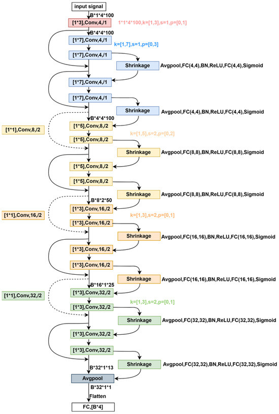
Figure 8.
The DRSN_CW with 18 layers. Our Actor network is influenced by the ResNet architecture, with differences in each layer’s convolutional kernels, stride, and channels, and an added shrinkage component. Specifically, the input data dimensions are [B, 1, 4, 100], where B represents the batch size, 4 indicates the four sensors, 100 signifies 100 time dimensions, and 1 denotes a reserved specific feature dimension. The data pass through a red-colored convolutional layer with a kernel size of [1, 3], a stride of 1, an input channel of 1, and an output channel of 4, resulting in data dimensions of [B, 4, 4, 100]. The setting for convolutional layers within the same-colored modules remains consistent. Every two convolutional modules combined with the shrinkage component form an RSBU-CW construction unit, where units of the same color share the same network settings.
3.4. Multi-Reward Mechanism
The multi-reward mechanism is a technology in reinforcement learning that is used to introduce and process multiple reward signals more effectively to enhance the learning and decision-making ability of agents. In some complex environments, a single reward signal may not fully express the diversity and complexity of the environment. Therefore, the introduction of multiple reward signals helps to provide more comprehensive and accurate training signals to improve the learning process and strategies. Compared with the previous method [26], the reward function is as follows:
We propose three other reward functions, as follows (34)–(36):
As shown in Formula (34), considering the mean square of four sensors over a period of time as the reward signal helps to reduce noise and fluctuations, making it smoother. This aids the agent to better understand the long-term trends of the environment, avoiding excessive interference from individual time-step rewards, and improving the stability and reliability of training. This approach also helps the agent to better consider long-term gains, reinforcing awareness of long-term planning and decision making rather than just focusing on immediate rewards. Averaging the reward signal also reduces the impact of environmental noise and randomness, enhancing the agent’s ability to handle complex situations. Overall, adopting the average value over a period of time as the reward function can improve training stability, smooth the reward signal, better consider long-term gains, and enhance the agent’s resistance to interference, effectively improving the training effectiveness of reinforcement learning models.
As shown in Formula (35), adopting the average of the root mean square (RMSE) of four sensors as the reward function has several advantages. Firstly, compared to extreme values, it exhibits higher robustness and stability. This means that the RMSE has less impact on the reward function when dealing with outliers, more evenly considers the overall characteristics of the data, and is less affected by extreme values. Additionally, the RMSE, being the square root of the mean square error, provides a more intuitive and understandable measurement. Compared to the mean square error, RMSE offers a more intuitive description of the error magnitude, emphasizing the size of the average error rather than the square of errors. It is noteworthy that the RMSE is less influenced by noise because it takes the square root of the mean error, resulting in a smoother signal. In certain situations, the RMSE better reflects real-world error scenarios, aligning more closely with the background and requirements of actual tasks. Lastly, due to its wide applicability, the RMSE as a reward function is suitable for various problems and scenarios and is commonly used in performance evaluation. In conclusion, selecting the RMSE as the reward function can provide a more robust, smooth, and understandable reward signal for training, helping the agent learn and adapt to the environment more effectively.
As shown in Formula (36), adopting the average of the variance of the four sensors as the reward function has unique advantages. It is a statistical measure of data dispersion, providing a metric for the diversity of behaviors exhibited by the agent in reinforcement learning. By evaluating the degree of behavioral variation, variance helps us to understand the consistency and diversity of the agent’s actions across different states. Additionally, variance also reflects the stability of the agent’s policy execution. A smaller variance may indicate more consistent and predictable behavioral patterns, while a larger variance implies more diversified actions taken across different states. Variance also indicates the agent’s sensitivity to environmental changes, and its adaptability to environmental changes can also be measured through variance. Overall, variance as a reward function provides a quantitative measure of the diversity, stability, and adaptability of the agent’s behavior in reinforcement learning. By assessing behavioral changes, variance helps us to gain insight into the agent’s learning process and strategy adjustments, guiding its optimization in complex environments.
We combine the influence of four different reward functions on the control strategy. Through comparative experiments, the optimal reward method is obtained, which can be seen in the subsequent analyses.
3.5. Priority Experience Replaying
The motivation of introducing priority experience replaying is to optimize the training process and solve the problems in traditional experience replaying. The traditional replaying method treats all empirical samples equally, but in fact, some experience is more important for model learning. Priority experience replaying introduces a mechanism that can focus more frequently on learning those experiences that have a greater impact on the model, thereby improving the efficiency of training and the performance of the model. In order to overcome these problems, we introduce a random sampling method [40] between pure greedy priority and uniform random sampling. We ensure that the probability of being sampled in the priority of a transition is monotonic, and that the probability is non-zero even for the transition of the lowest priority. Specifically, we define the probability i of the sampling transition as follows:
where > 0 is the priority of conversion i. The index determines how much priority is used, and = 0 corresponds to the uniform case.
The first variant we consider is a direct, proportional priority, where , and is a small positive constant that prevents the transition edge from not being revisited once the error is zero. The second variant is an indirect, rank-based priority, where , and is the level of data i sorted by in the experience pool. In this case, becomes a power-law distribution with exponent . In error, both distributions are monotonic, but the latter is more robust because it is not sensitive to outliers.
In order to effectively sample from the distribution in Equation (37), the complexity cannot depend on the capacity of the empirical pool. For rank-based variants, we can approximate the cumulative density function using a piecewise linear function with k equal probability segments. The segment boundaries can be calculated in advance (they only change when or changes). At runtime, we sample a fragment and then uniformly sample it in the transformation. This is especially effective when combined with minibatch-based learning algorithms: selecting as the size of the minibatch and sampling a transition from each segment precisely is a form of stratified sampling that has the additional advantage of balancing the minibatch. The proportional variables are different, and also allow effective implementation based on the “sum-tree” data structure (where each node is the sum of its child nodes, and the priority is the leaf node), which can be effectively updated and sampled.
4. Experimental Results and Discussion
This chapter mainly introduces some comparative experiments and ablation experiments, including lightweight comparative experiments, priority experience replaying comparative experiments, optimal reward function combination, demonstrating the feasibility of this lightweight method, alleviating overestimation experiments, and relevant comparative experiments.
4.1. Lightweight Comparative Experiment
Under narrowband white-noise excitation ranging from 0 to 100 Hz, with 0.3 s of data for root mean square calculation, Table 1 illustrates the setup of platform simulators for vibration control using our DRSL-MPER algorithm and under the DDPG framework using fully connected (FC), CNN, GoogleNet, and LSTM methods. The first column indicates various algorithms; the second column shows the values of the vibration signal before being controlled, measured in volts (V); the third column displays the values of the vibration signal after being controlled, also measured in volts (V); the fourth column indicates the parameter quantity, measured as a number (N), representing the total number of weight parameters and bias parameters in the neural network; and the fifth column represents the degree of vibration signal reduction, measured in decibels (dB).

Table 1.
Lightweight comparison experiment. Under the same experimental conditions, the method proposed in this paper achieves better control effectiveness with fewer parameters. The first row represents the algorithm, the second row displays the vibration signal values before being controlled, the third row shows the vibration signal values after being controlled, the fourth row indicates the parameter quantity, and the fifth row represents the reduction in vibration control, measured in dB.
Reference [26] proposed the fully connected network and DDPG framework as the primary points of comparison, detailing their parameters and vibration reduction levels. Considering the prevalent use of fully connected network methods in the current domain, we introduced methods such as convolutional neural networks (CNNs), GoogLeNet, and Long Short-Term Memory networks (LSTMs) to expand the experimental scope; relevant parameters and vibration reduction levels are listed in the table above. Under narrowband white-noise excitation ranging from 0 to 100 Hz, our DRSL-MPER method achieved a vibration reduction of up to 20.240 dB with a reduction in parameters by more than 7.5 times. A greater reduction indicates better vibration control effectiveness.
4.2. Comparison between Prioritized Experience Replaying and Non-Prioritized Experience Replaying
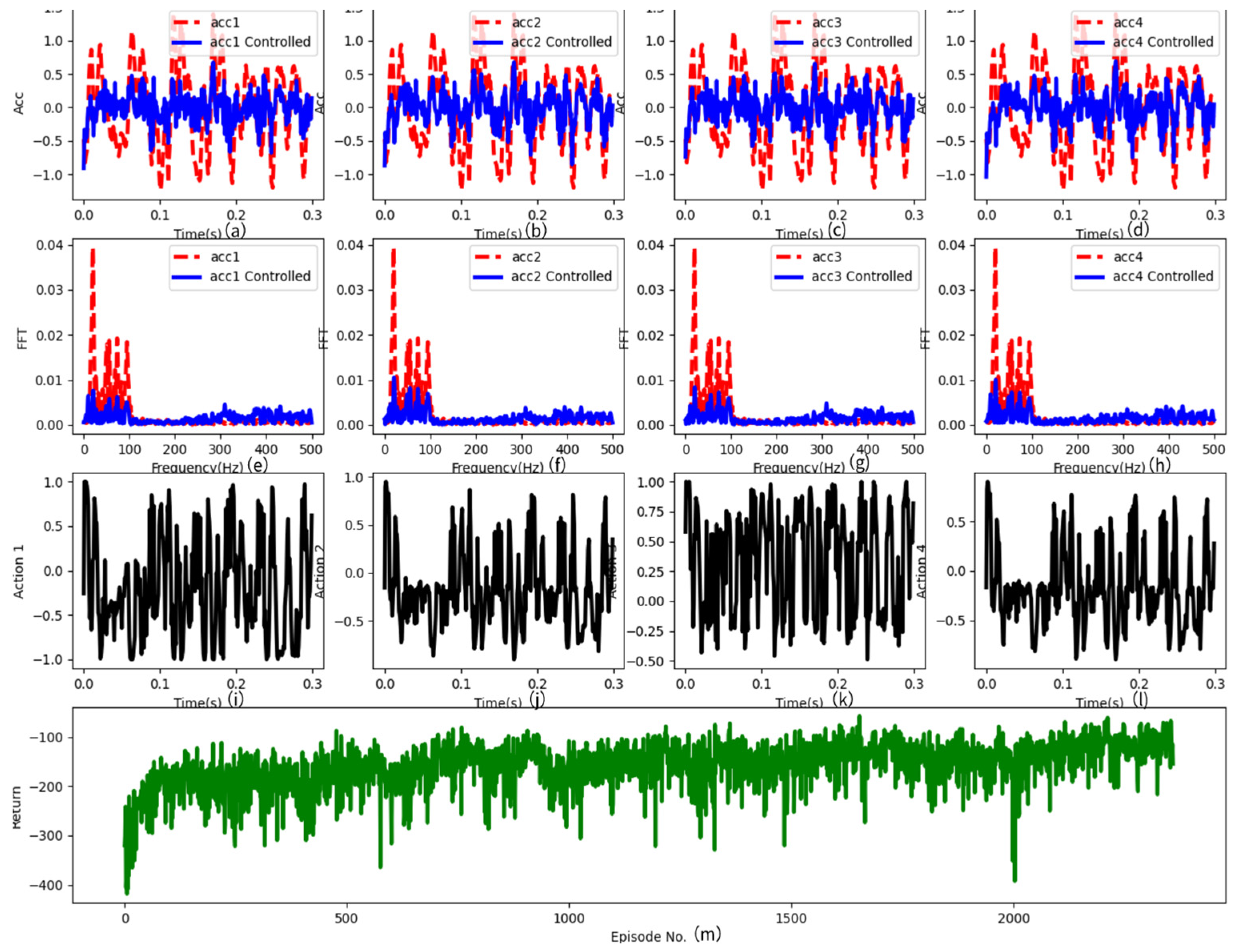
To clearly present the experimental results, we visualized the time-domain signals before and after the control, the frequency-domain signals obtained through Fourier transformation, the action-value signals, and the reward values. Similar experimental results are also summarized here for subsequent experiments. As shown in Figure 9, the first row (a)–(d) displays the time-domain control signals, where the x-axis represents time and the y-axis represents the control signal in volts (V); the second row (e)–(f) illustrates the frequency-domain control signals, with the x-axis representing the frequency range in Hz and the y-axis indicating the values after Fourier transformation (FFT); the third row (i)–(l) represents the action values of the agent; and the fourth row (m) represents the reward values. In the latter two rows, the x-axis represents time and the y-axis represents the magnitude of the action values or the number of rounds for the reward values. Although reward values may be negative, higher values indicate better control effectiveness, albeit not absolutely. These visualizations help demonstrate the performance of the algorithm during the control process and the variations in signals.
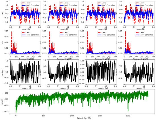
Figure 9.
The control signal, Fourier transform signal, action signal, and reward value obtained through experimentation. The first row (a–d) exhibits the time-domain signals from four sensors, where the x-axis denotes time steps (300 time points were captured in the experiment, scaled to the range [0.0, 0.3] by dividing by 1000), while the y-axis represents the original signal in red and the controlled signal in blue. Clearly, through effective algorithmic control, the blue signals gradually shift towards zero. The second row (e–h) displays the frequency-domain signals obtained by performing Fourier transforms on the data from the first row for each sensor. It is noticeable that the red non-controlled signals primarily concentrate within the range of [0–100] Hz, with fewer signals in other frequency domains. However, the controlled blue signals exhibit a significant reduction in the frequency domain. The third row (i–l) illustrates the control signals emitted by the controller. The x-axis corresponds to the same time steps as in the first row, while the y-axis represents control signal values within the range of [−1.0, 1.0], due to the final network layer of the controller utilizing the tanh activation function. The final row (m) represents the reward values, where the x-axis indicates the episode, and the y-axis depicts the reward value for each episode.
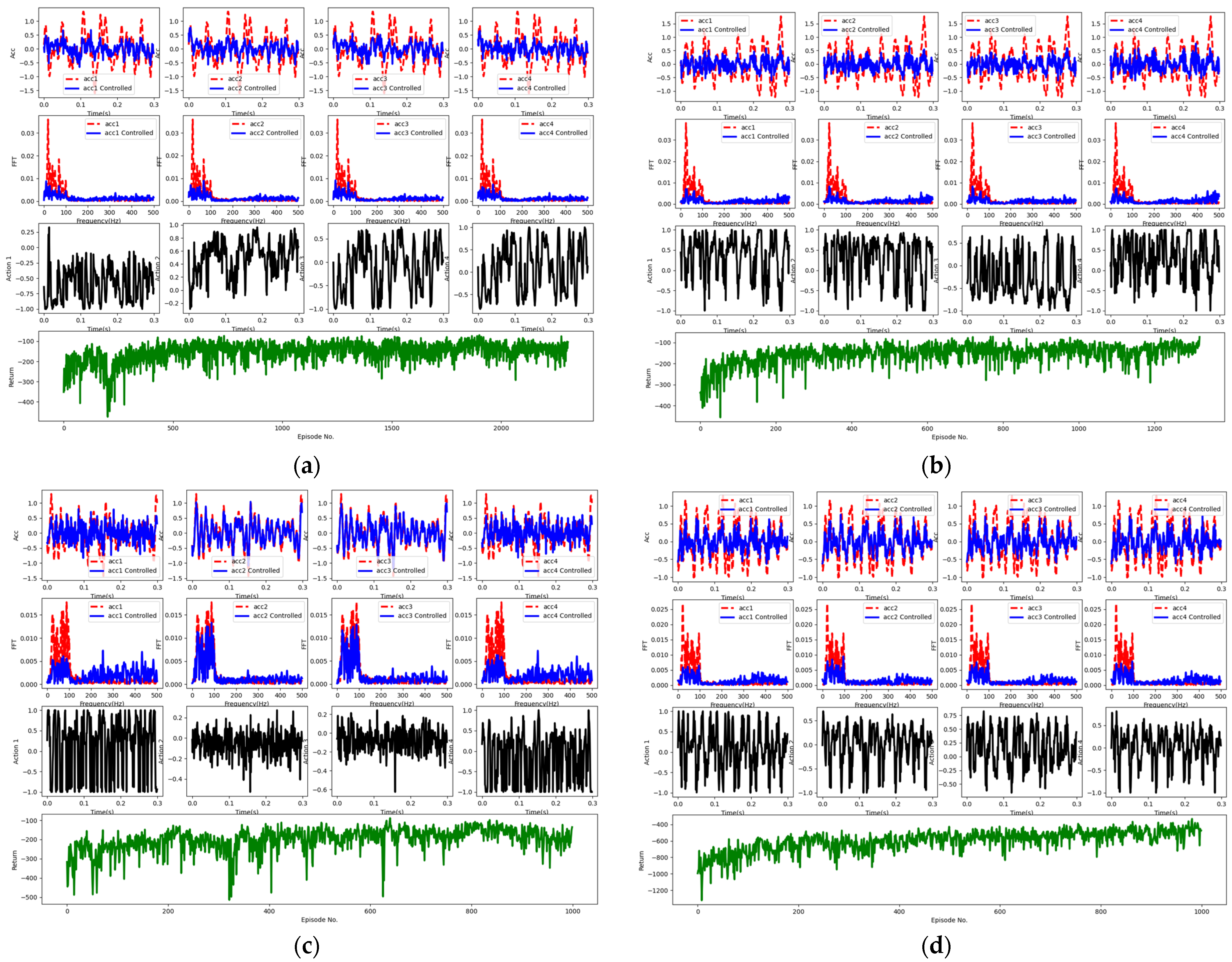
Figure 10 illustrates how the utilization of prioritized experience replay enhances the convergence speed and control effectiveness under both DRSN and TD3 reinforcement learning frameworks. Under narrowband white-noise excitation ranging from 0 to 100 Hz, Figure 10a shows that optimal performance is reached after approximately 2500 iterations, while Figure 10b shows that the same is achieved after only 1300 iterations, showcasing a convergence speed close to twice that of non-experience replay. To validate the effectiveness of prioritized experience replay, we conducted training with and without prioritized experience replay for 1000 episodes, as shown in Figure 10c,d, respectively. Through calculations, Figure 10c demonstrates a vibration reduction of 7.9 dB without prioritized experience replay, while Figure 10d indicates a reduction of up to 12.5 dB with prioritized experience replay. These contrasting experiments reveal that training with prioritized experience replay is more stable and exhibits higher data efficiency.
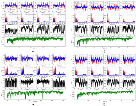
Figure 10.
In this figure, (a) depicts the network with DRSN and TD3 framework without prioritized experience replay, while (b) shows the network with DRSN and TD3 framework with prioritized experience replay; (c) represents training without prioritized experience replay for 1000 episodes, and (d) illustrates training with prioritized experience replay for 1000 episodes.
4.3. Optimal Reward Function Combination
To explore the most suitable combination of reward functions, we synthesized the original reward function, variance, root mean square, and mean from [26], as detailed in Table 2. Under the conditions of employing both DRSN methods in the Actor and Critic networks, along with the application of prioritized experience replay, we experimented with various combinations of reward functions and drew conclusions. When used individually, the original reward function performed the poorest compared to variance, root mean square, and mean. Among the combined functions, as highlighted in red, the combination with the root mean square exhibited the most favorable effects. However, the data highlighted in blue indicated that the original reward function might have a detrimental impact on the combination, often leading to decreased performance. Therefore, we recommend using the combination of root mean square and mean values, which performs better in most cases, resulting in the maximum reduction of up to 20.240 dB.

Table 2.
In the cases of TD3 and DRSN, with combinations of multiple reward functions, we denote the variance, mean square value, root mean square, and original method as V, MSV, RMS, and OM, respectively. In the same experimental setting, the OM reward function exhibits negative effects, while the root mean square generates positive impacts.
4.4. Demonstrating the Feasibility of This Lightweight Method
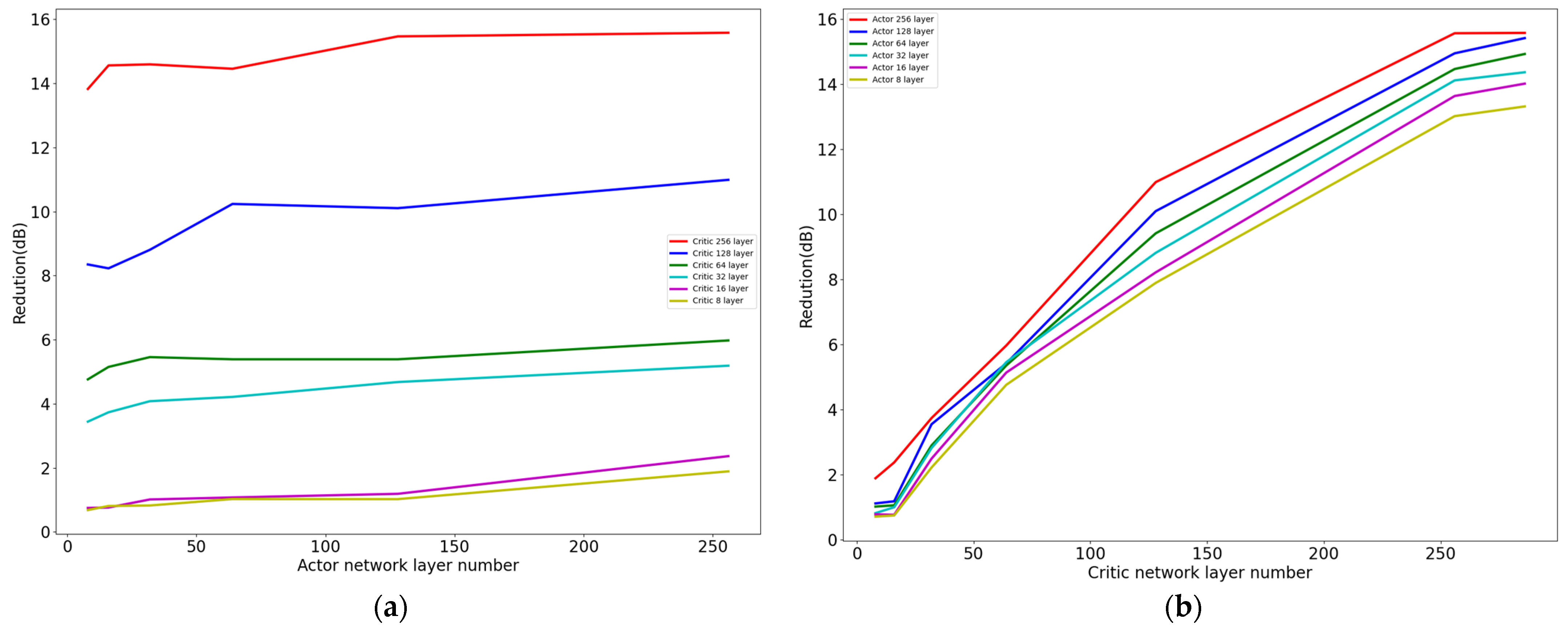
To verify the feasibility of the lightweight method, we compared the performance of the fully connected networks under different settings. In this experiment, the Actor network structure was [400, x, x, 4], and the Critic network structure was [400, x, x, 1], where x is an integer. For both Figure 11a,b, we gradually increased the size of the neural network’s intermediate layers from 8 to 16, to 32, to 64, to 128, doubling each layer. In Figure 11a, the different colors represent different numbers of intermediate layers in the Critic network. As the number of intermediate layers in the Actor network increased, the effectiveness of vibration control gradually improved. In Figure 11b, the different colors represent different numbers of intermediate layers in the Actor network. As the number of intermediate layers in the Critic network increased, the effectiveness of vibration control also increased. In our DRSL-MPER method, the Actor and Critic networks used the same network structure, with parameter counts of 22,584 and 44,970, respectively, achieving a control effect of 20.24 dB. In contrast, when the intermediate layer size was 64, the Actor had 30,084 parameters, the Critic had 59,906 parameters, and the control effect reached 5.358 dB, which is close to our method in terms of the parameter count. This indicates that DRSL-MPER increased the damping effect by 14.882 dB with fewer parameters. In comparison, the best control effect occurred when the intermediate layers of both the Actor and Critic were 256, achieving a control effect of 15.57 dB. The Actor had 169,476 parameters, the Critic had 337,922 parameters, and DRSL-MPER improved the control effect by 4.67 dB with only 13% of the parameters of the 256-layer network. These results clearly demonstrate the significant advantages of our lightweight network in relation to both its effectiveness and its parameter count.
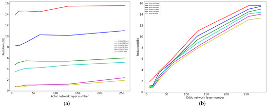
Figure 11.
Impact diagrams of different Actor/Critic parameters on vibration control. Through experiments with varying numbers of FC layers in the Actor/Critic networks, this study demonstrates the superiority of the proposed method in terms of both the parameter efficiency and control effectiveness. (a) With fixed Critic parameters, the effect of Actor parameter variation on vibration control. Here, the Actor network structure is [400, x, x, 4], where the horizontal x-axis represents a reduction in Actor network layers, and the vertical axis denotes the control rate (percentage), the ratio of controlled to uncontrolled states before and after the control process. (b) With fixed Actor parameters, the effect of Critic parameter variation on vibration control. The Critic network structure is [400, x, x, 1], where the horizontal x-axis represents a reduction in Critic network layers, and the vertical axis denotes the control rate (percentage), the ratio of controlled to uncontrolled states before and after the control process.
4.5. Alleviating Overestimation Experiments
This study adopts the TD3 algorithm, aiming to alleviate the common problem of value function overestimation in the Actor–Critic architecture. The Actor–Critic algorithm combines value function approximation (Critic) and policy approximation (Actor), where the Critic is responsible for estimating state-value or action-value functions, and the Actor updates the policy based on these estimates. However, due to errors in function approximation, nonlinear approximations, and limited sample sizes, the Critic network in the Actor–Critic algorithm often overestimates the true value, leading to suboptimal or even unstable policies. This experiment compared the DDPG framework with the TD3 framework. We recorded their Q-values and true values across 10,000 episodes. In Figure 12, the horizontal axis represents the episodes, and the vertical axis represents the magnitude of Q-values. Figure 12a shows the Q-values and true values of DDPG. It is observed that the Q-values are consistently higher than the true values, which also proves the existence of overestimation in the AC framework. Next, we introduced the TD3 framework, and in Figure 12b, it is shown that the Q-values of TD3 overlap significantly with the true values, indicating that the TD3 framework effectively alleviates the overestimation problem.


Figure 12.
Comparison between the DDPG and TD3 frameworks, confirming the overestimation phenomenon in DDPG. The TD3 framework leverages the minimum value from two networks, mitigating the overestimation issue inherent in the DDPG framework. (a) The Q-values and ground-truth values for DDPG. (b) The Q-values and ground-truth values for TD3.
4.6. Relevant Comparative Experiments
4.6.1. Relevant Comparative Experiments for Lightweightness
In Section 4.1, we emphasized the feasibility and advantages of the lightweighting approach. To gain further insights into the impact of lightweighting experiments on different modules and parameter quantities, we conducted comparative experiments specifically focusing on the Actor, Critic, and reinforcement learning frameworks. The baseline model comprised Actor and Critic networks with fully connected layers of a 256 size (FC256), utilizing the DDPG reinforcement learning framework. In Table 3, the first column represents the Actor network structure, the second column denotes the Critic network structure, the third column indicates the reinforcement learning framework, the fourth column details the total parameter count, and the fifth column presents the reduction, where smaller values are preferred. The experimental findings reveal that the DRSN performs better than FC256 in both the Actor and Critic networks. Additionally, despite the TD3 algorithm increasing the parameter count under the same network structure, there is a significant enhancement in the control effectiveness, and the increased parameter count remains within an acceptable range. Furthermore, we observed that improvements in the Critic network have a more pronounced impact on control effectiveness compared to improvements in the Actor network. The best vibration reduction can reach up to 20.240 dB.

Table 3.
The impact of Actor and Critic networks as well as the reinforcement learning framework in the lightweighting comparative experiments. By controlling the Actor network, Critic network, RL framework, and parameter count, it was observed that in both the DDPG and TD3 frameworks, the influence of the Critic network on control effectiveness outweighs that of the Actor network.
4.6.2. Relevant Comparative Experiments for Prioritized Experience Replay
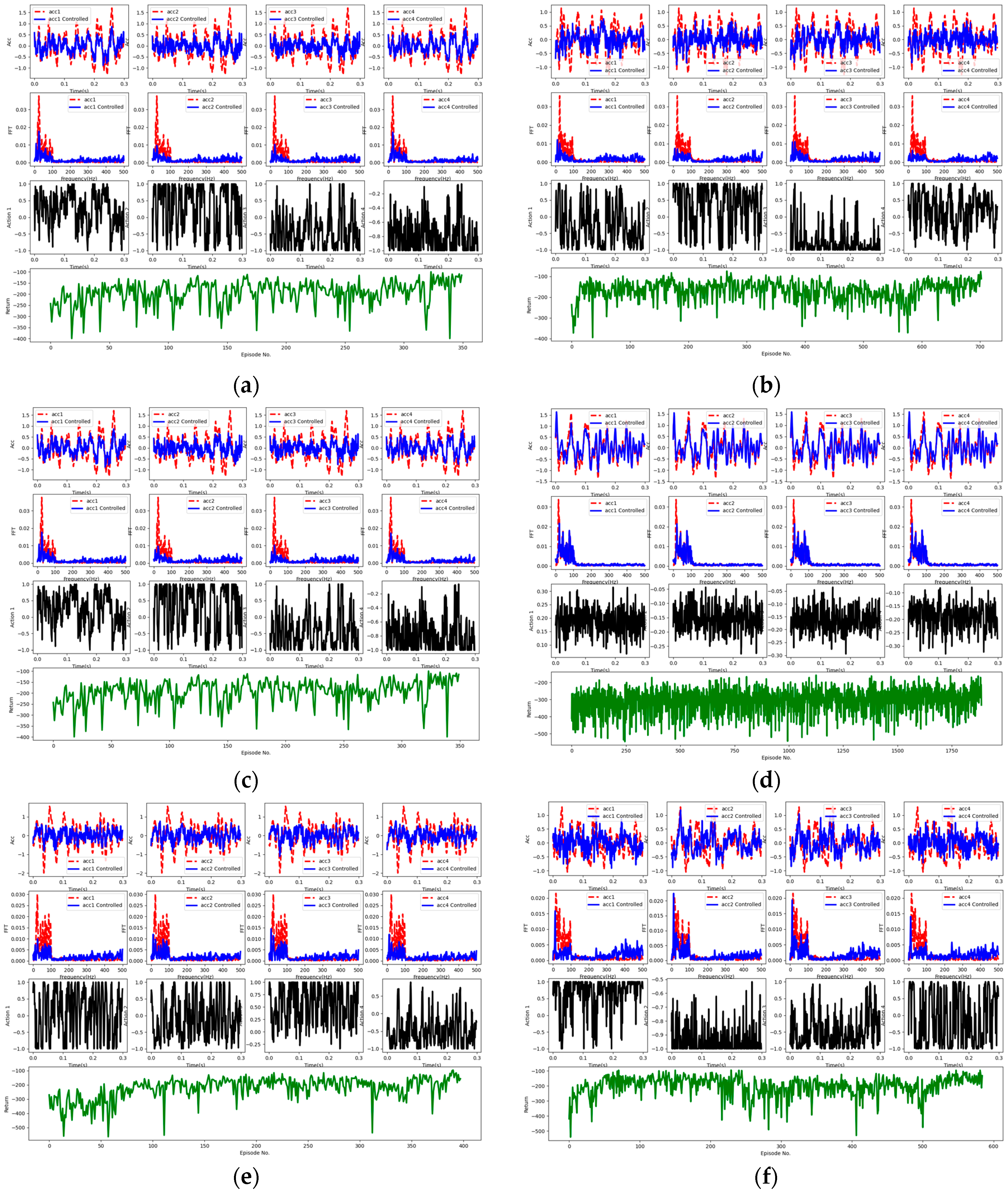
In Section 4.2, we emphasized the superiority of prioritized experience replay under the DRSN and TD3 reinforcement learning frameworks. To further demonstrate its generalizability, we conducted multiple experiments. Figure 13a–f demonstrate the enhanced data utilization efficiency by prioritized experience replay under both fully connected and DRSN conditions. Both (a) and (b) adopt the DDPG framework under the DRSN. In (a), the number of rounds taken to reach convergence under prioritized experience replay is around 350, while in (b), convergence is achieved at approximately 700 rounds. Both (c) and (d) utilize the TD3 framework under the fully connected network. In (c), the number of rounds taken to achieve convergence under prioritized experience replay is approximately 350, while in (f), convergence is not reached even after 1750 rounds. Both (e) and (f) adopt the DDPG framework under the fully connected network. In (e), the number of rounds taken to reach convergence under prioritized experience replay is approximately 400, with a vibration reduction of 9.25 dB, while in (f), convergence is achieved at approximately 600 rounds, with a vibration reduction of 3.53 dB. Both the DDPG and TD3 reinforcement learning algorithms exhibit effectiveness, highlighting that prioritized experience replay is not constrained by specific neural network architectures or reinforcement learning frameworks. It fundamentally enhances data utilization efficiency, proving its generalizability. While Figure 13a–f differ in the network structures, Figure 13 showcases more pronounced control effects, indirectly validating the feasibility of the DRSN method.

Figure 13.
(a) Prioritized experience replay with the DRSN under the DDPG framework. (b) Non-prioritized experience replay with the DRSN under the DDPG framework. (c) Prioritized experience replay with the fully connected network under the TD3 framework. (d) Non-prioritized experience replay with fully connected network under the TD3 framework. (e) Prioritized experience replay with the fully connected network under the DDPG framework. (f) Non-prioritized experience replay with the fully connected network under the DDPG framework.
4.6.3. Relevant Comparative Experiments for the Optimal Reward Functions
In Section 4.3, we discussed the optimal reward function combinations within the DRSN and TD3 frameworks. To further investigate the applicability of these reward functions, we conducted additional studies under baseline experimental conditions, namely within the FC256 and DDPG frameworks. In Table 2 and Table 4, similar trends can be observed. The data points highlighted in red indicate the superior effectiveness of combining the root mean square function. Conversely, the data points highlighted in blue suggest that the original reward function may adversely impact the combined performance, often resulting in inferior outcomes. Therefore, we recommend employing a combination of the root mean square and mean square value functions.

Table 4.
In the cases of DDPG and FC256, with combinations of multiple reward functions, we denote the variance, mean square value, root mean square, and original method as V, MSV, RMS, and OM, respectively. We assign a rating to the reward functions, utilizing measurements before and after the control process.
4.6.4. Ablation Experiments
In this section, ablation experiments were conducted on a narrowband white-noise excitation dataset ranging from 0 to 100 Hz to verify the effectiveness of the proposed modules. Table 5 illustrates the various methods studied alongside average convergence episodes, parameters, and reduction levels. We noticed that compared to the baseline, the introduction of the DRSN not only reduced the parameters by approximately 6.5 times but also increased the damping effect by 2.6 dB. Furthermore, the inclusion of the RMSV+RMS reward function resulted in an additional damping improvement of 0.882 dB. Subsequently, the introduction of prioritized experience replay reduced the average convergence rounds to 634 times. Lastly, the integration of the TD3 framework, although it increased the parameters and rounds slightly, did not affect the overall performance, yet achieved the peak control effectiveness of 20.240 dB.

Table 5.
In the ablation experiments, OM, MSV, RMS, and PER, respectively, represent the original method, mean square value, root mean square, and prioritized experience replay. The ablation experiments demonstrated the efficiency of DRSN lightweighting and the MSV + RMS combination function, with a faster convergence speed for PER.
5. Conclusions
This work introduces a multi-reward mechanism to assist lightweight networks in finding nearly optimal control strategies. Additionally, a prioritized experience replay mechanism is introduced to assign priority to data, accelerating the convergence speed of neural networks and enhancing data utilization efficiency. The incorporation of a deep residual contraction network achieves adaptive denoising and lightweighting of the neural networks, making it currently one of the most preferable methods under real-world conditions. In these experiments, we utilized a continuous length of 100 time points from each sensor as the state, and our plans for future research involve further exploration of appropriate time point lengths for the sensors. Furthermore, the consideration of convolutional hyperparameters is also deemed worthwhile. Future research directions should encompass migrating this method to force control and magnetic control, as well as registration and classification tasks in medical imaging. Through these efforts, we aim to continuously optimize and advance the application of this method in various domains.
Author Contributions
Conceptualization, Y.S. and C.H.; methodology, Y.S.; software, C.H.; valiadation, L.Q., B.X. and W.L.; formal analysis, L.Q.; investigation, B.X.; resources, W.L.; data curation, Y.S.; writing—original draft preparation, C.H.; writing—review and editing, Y.S.; visualization, C.H.; supervision, L.Q.; project administration, W.L.; funding acquisition, B.X. All authors have read and agreed to the published version of the manuscript.
Funding
This research was funded in part by the National Natural Science Foundation of China 62276040, 62331008, National Major Scientific Research Instrument Development Project of China 62027827, National Natural Science Foundation of Chongqing CSTB2022NSCQ-MSX0436.
Institutional Review Board Statement
Not applicable.
Informed Consent Statement
Not applicable.
Data Availability Statement
The original contributions presented in the study are included in the article, further inquiries can be directed to the corresponding authors.
Conflicts of Interest
The authors declare no conflicts of interest.
References
- Ab Talib, M.H.; Mat Darus, I.Z.; Mohd Samin, P.; Mohd Yatim, H.; Ardani, M.I.; Shaharuddin, N.M.R.; Hadi, M.S. Vibration control of semi-active suspension system using PID controller with advanced firefly algorithm and particle swarm optimization. J. Ambient. Intell. Humaniz. Comput. 2021, 12, 1119–1137. [Google Scholar] [CrossRef]
- Li, W.; Yang, Z.; Li, K.; Wang, W. Hybrid feedback PID-FxLMS algorithm for active vibration control of cantilever beam with piezoelectric stack actuator. J. Sound Vib. 2021, 509, 116243. [Google Scholar] [CrossRef]
- Wang, L.; Liu, J.; Yang, C.; Wu, D. A novel interval dynamic reliability computation approach for the risk evaluation of vibration active control systems based on PID controllers. Appl. Math. Model. 2021, 92, 422–446. [Google Scholar] [CrossRef]
- Zhang, Q.; Yang, Z.; Wang, C.; Yang, Y.; Zhang, R. Intelligent control of active shock absorber for high-speed elevator car. Proc. Inst. Mech. Eng. Part C J. Mech. Eng. Sci. 2019, 233, 3804–3815. [Google Scholar] [CrossRef]
- Tian, J.; Guo, Q.; Shi, G. Laminated piezoelectric beam element for dynamic analysis of piezolaminated smart beams and GA-based LQR active vibration control. Compos. Struct. 2020, 252, 112480. [Google Scholar] [CrossRef]
- Takeshita, A.; Yamashita, T.; Kawaguchi, N.; Kuroda, M. Fractional-order LQR and state observer for a fractional-order vibratory system. Appl. Sci. 2021, 11, 3252. [Google Scholar] [CrossRef]
- Lu, X.; Liao, W.; Huang, W.; Xu, Y.; Chen, X. An improved linear quadratic regulator control method through convolutional neural network–based vibration identification. J. Vib. Control. 2021, 27, 839–853. [Google Scholar] [CrossRef]
- Niu, W.; Zou, C.; Li, B.; Wang, W. Adaptive vibration suppression of time-varying structures with enhanced FxLMS algorithm. Mech. Syst. Signal Process. 2019, 118, 93–107. [Google Scholar] [CrossRef]
- Puri, A.; Modak, S.V.; Gupta, K. Modal filtered-x LMS algorithm for global active noise control in a vibro-acoustic cavity. Mech. Syst. Signal Process. 2018, 110, 540–555. [Google Scholar] [CrossRef]
- Seba, B.; Nedeljkovic, N.; Paschedag, J.; Lohmann, B. H∞ Feedback control and Fx-LMS feedforward control for car engine vibration attenuation. Appl. Acoust. 2005, 66, 277–296. [Google Scholar] [CrossRef]
- Carlucho, I.; de Paula, M.; Wang, S.; Petillot, Y.; Acosta, G. Adaptive low-level control of autonomous underwater vehicles using deep reinforcement learning. Robot. Auton. Syst. 2018, 107, 71–86. [Google Scholar] [CrossRef]
- Pane, Y.P.; Nageshrao, S.P.; Kober, J.; Babuška, R. Reinforcement learning based compensation methods for robot manipulators. Eng. Appl. Artif. Intell. 2019, 78, 236–247. [Google Scholar] [CrossRef]
- Silver, D.; Hubert, T.; Schrittwieser, J.; Antonoglou, I.; Lai, M.; Guez, A.; Lanctot, M.; Sifre, L.; Kumaran, D.; Graepel, T.; et al. A general reinforcement learning algorithm that masters chess, shogi, and Go through self-play. Science 2018, 362, 1140–1144. [Google Scholar] [CrossRef]
- Ye, D.; Liu, Z.; Sun, M.; Shi, B.; Zhao, P.; Wu, H.; Yu, H.; Yang, S.; Wu, X.; Guo, Q.; et al. Mastering complex control in MOBA games with deep reinforcement learning. arXiv 2020, arXiv:1912.09729. [Google Scholar] [CrossRef]
- Degrave, J.; Felici, F.; Buchli, J.; Neunert, M.; Tracey, B.; Carpanese, F.; Ewalds, T.; Hafner, R.; Abdolmaleki, A.; de las Casas, D.; et al. Magnetic control of tokamak plasmas through deep reinforcement learning. Nature 2022, 602, 414–419. [Google Scholar] [CrossRef] [PubMed]
- Li, Z.; Chu, T.; Kalabić, U. Dynamics-enabled safe deep reinforcement learning: Case study on active suspension control. In Proceedings of the 2019 IEEE Conference on Control Technology and Applications (CCTA), Hong Kong, China, 19–21 August 2019; pp. 585–591. [Google Scholar]
- Zhao, F.; You, K.; Song, S.; Zhang, W.; Tong, L. Suspension regulation of medium-low-speed maglev trains via deep reinforcement learning. IEEE Trans. Artif. Intell. 2021, 2, 341–351. [Google Scholar] [CrossRef]
- Ding, Z.; Song, C.; Xu, J.; Dou, Y. Human-Robot Interaction System Design for Manipulator Control Using Reinforcement Learning. In Proceedings of the 2021 36th Youth Academic Annual Conference of Chinese Association of Automation (YAC), Nanchang, China, 28–30 May 2021; pp. 660–665. [Google Scholar]
- Baselizadeh, A.; Khaksar, W.; Torresen, J. Motion Planning and Obstacle Avoidance for Robot Manipulators Using Model Predictive Control-based Reinforcement Learning. In Proceedings of the 2022 IEEE International Conference on Systems, Man, and Cybernetics (SMC), Prague, Czech Republic, 9–12 October 2022; pp. 1584–1591. [Google Scholar]
- Vatsal, V.; Purushothaman, B. Reinforcement Learning of Whole-Body Control Strategies to Balance a Dynamically Stable Mobile Manipulator. In Proceedings of the 2021 Seventh Indian Control Conference (ICC), Virtually, 20–22 December 2021; pp. 335–340. [Google Scholar]
- Park, J.-E.; Lee, J.; Kim, Y.-K. Design of model-free reinforcement learning control for tunable vibration absorber system based on magnetorheological elastomer. Smart Mater. Struct. 2021, 30, 055016. [Google Scholar] [CrossRef]
- Yuan, R.; Yang, Y.; Su, C.; Hu, S.; Zhang, H.; Cao, E. Research on vibration reduction control based on reinforcement learning. Adv. Civ. Eng. 2021, 2021, 7619214. [Google Scholar] [CrossRef]
- Qiu, Z.; Chen, G.; Zhang, X. Trajectory planning and vibration control of translation flexible hinged plate based on optimization and reinforcement learning algorithm. Mech. Syst. Signal Process. 2022, 179, 109362. [Google Scholar] [CrossRef]
- Qiu, Z.; Chen, G.; Zhang, X. Reinforcement learning vibration control for a flexible hinged plate. Aerosp. Sci. Technol. 2021, 118, 107056. [Google Scholar] [CrossRef]
- Qiu, Z.; Yang, Y.; Zhang, X. Reinforcement learning vibration control of a multi-flexible beam coupling system. Aerosp. Sci. Technol. 2022, 129, 107801. [Google Scholar] [CrossRef]
- Feng, X.; Chen, H.; Wu, G.; Zhang, A.; Zhao, Z. A New Vibration Controller Design Method Using Reinforcement Learning and FIR Filters: A Numerical and Experimental Study. Appl. Sci. 2022, 12, 9869. [Google Scholar] [CrossRef]
- He, K.; Zhang, X.; Ren, S.; Sun, J. Deep residual learning for image recognition. In Proceedings of the IEEE Conference on Computer Vision and Pattern Recognition, Las Vegas, NV, USA, 27–30 June 2016; pp. 770–778. [Google Scholar]
- Howard, A.G.; Zhu, M.; Chen, B.; Kalenichenko, D.; Wang, W.; Weyand, T.; Andreetto, M.; Adam, H. Mobilenets: Efficient convolutional neural networks for mobile vision applications. arXiv 2017, arXiv:1704.04861. [Google Scholar]
- Zhang, X.; Zhou, X.; Lin, M.; Sun, J. Shufflenet: An extremely efficient convolutional neural network for mobile devices. In Proceedings of the IEEE Conference on Computer Vision and Pattern Recognition, Salt Lake City, UT, USA, 18–23 June 2018; pp. 6848–6856. [Google Scholar]
- Zhao, M.; Zhong, S.; Fu, X.; Tang, B.; Pecht, M. Deep residual shrinkage networks for fault diagnosis. IEEE Trans. Ind. Inform. 2019, 16, 4681–4690. [Google Scholar] [CrossRef]
- Sutton, R.S.; McAllester, D.; Singh, S.; Mansour, Y. Policy gradient methods for reinforcement learning with function approximation. Adv. Neural Inf. Process. Syst. 1999, 12, 1057–1063. [Google Scholar]
- Watkins, C.J.; Dayan, P. Q-learning. Mach. Learn. 1992, 8, 279–292. [Google Scholar] [CrossRef]
- Konda, V.; Tsitsiklis, J. Actor-critic algorithms. Adv. Neural Inf. Process. Syst. 1999, 13, 1008–1014. [Google Scholar]
- Lillicrap, T.P.; Hunt, J.J.; Pritzel, A.; Heess, N.; Erez, T.; Tassa, Y.; Silver, D.; Wierstra, D. Continuous control with deep reinforcement learning. arXiv 2015, arXiv:1509.02971. [Google Scholar]
- Haarnoja, T.; Zhou, A.; Hartikainen, K.; Tucker, G.; Ha, S.; Tan, J.; Kumar, V.; Zhu, H.; Gupta, A.; Abbeel, P. Soft actor-critic algorithms and applications. arXiv 2018, arXiv:1812.05905. [Google Scholar]
- Fujimoto, S.; Hoof, H.; Meger, D. Addressing function approximation error in actor-critic methods. In Proceedings of the International Conference on Machine Learning, Vienna, Austria, 10–15 July 2018; pp. 1587–1596. [Google Scholar]
- Hayes, M.H. Statistical Digital Signal Processing and Modeling; John Wiley & Sons: Hoboken, NJ, USA, 1996. [Google Scholar]
- Donoho, D.L. De-noising by soft-thresholding. IEEE Trans. Inf. Theory 1995, 41, 613–627. [Google Scholar] [CrossRef]
- Isogawa, K.; Ida, T.; Shiodera, T.; Takeguchi, T. Deep shrinkage convolutional neural network for adaptive noise reduction. IEEE Signal Process. Lett. 2017, 25, 224–228. [Google Scholar] [CrossRef]
- Schaul, T.; Quan, J.; Antonoglou, I.; Silver, D. Prioritized experience replay. arXiv 2015, arXiv:1511.05952. [Google Scholar]
Disclaimer/Publisher’s Note: The statements, opinions and data contained in all publications are solely those of the individual author(s) and contributor(s) and not of MDPI and/or the editor(s). MDPI and/or the editor(s) disclaim responsibility for any injury to people or property resulting from any ideas, methods, instructions or products referred to in the content. |
© 2024 by the authors. Licensee MDPI, Basel, Switzerland. This article is an open access article distributed under the terms and conditions of the Creative Commons Attribution (CC BY) license (https://creativecommons.org/licenses/by/4.0/).

