Article

Design and Experimentation of Tensegrity Jumping Robots

by
Guoxin Tang
,
Qi Yang
* and
Binbin Lian
Key Lab for Mechanism Theory and Equipment Design of Ministry of Education, Tianjin University, Tianjin 300350, China
*
Author to whom correspondence should be addressed.
Appl. Sci. 2024, 14(9), 3947; https://doi.org/10.3390/app14093947
Submission received: 15 April 2024 / Revised: 2 May 2024 / Accepted: 3 May 2024 / Published: 6 May 2024
(This article belongs to the Section Robotics and Automation)

Abstract

:
Jumping robots possess the capability to surmount formidable obstacles and are well-suited for navigating through complex terrain environments. However, most of the existing jumping robots face challenges in achieving stable jumping and they also have low energy utilization efficiency, which limits their practical applications. In this work, a two-module jumping robot based on tensegrity structure is put forward. Firstly, the structural design and jumping mechanism of the robot are elaborated in the article. Then, dynamic models, including the two modules’ simultaneous jumping and step-up jumping process of the robot, are established utilizing the Lagrange dynamic modeling method. On this basis, the effects of parameters, including the stiffness of elastic cables and the initial tilt angle of the robot, on the jumping performance of the robot can be obtained. Finally, simulations are carried out and a prototype is developed to verify the rationality of the tensegrity-based jumping robot proposed in this work. The experiment results show that our jumping robot can achieve a stable jumping process and the step-up jumping of each module of the prototype can have higher energy efficiency than that of simultaneous jumping of each module, which enables the robot a better jumping performance. This research serves as a valuable reference for the design and analysis of jumping robots.

1. Introduction

In recent years, the rapid development of science and technology has ushered in an unprecedented boom in robotics in a variety of fields [1,2,3,4,5]. Robots, as intelligent devices capable of simulating and replacing humans in performing diverse tasks, have been widely used in manufacturing, healthcare, military defense, and many other fields [6,7,8,9,10].
Most traditional mobile robots rely on wheels or leg structures for mobility but in some specific conditions, these mobility methods are out of reach [11,12,13]. In complex in conditions such as irregular terrain, steep mountains, or disaster sites, the mobility of conventional robots is greatly limited due to rugged terrain and obstacles all over the place [14,15,16]. Among them, jumping robots attracted many researchers due to their excellent mobility and adaptability [17]. Jumping robots excel in complex environments due to their unique locomotion. They are widely used in fields like space exploration, disaster rescue, and military applications, which makes jumping robots an important development direction for future robotics technology with a broad application outlook [18,19,20].
Jumping robots, a special type in the field of robotics, are endowed with high maneuverability and obstacle-crossing capabilities due to aerial jumping ability. Yan He and Zhu Xingyue of Shanghai Jiao Tong University have recently developed a small lunar surface jumping robot to study robotic jumps in lunar surface situations [21]. Ruide Yun, Zhiwei Liu, and others at Beihang University have recently developed a millimeter-sized jumping micro-robot to study the crawling and jumping of the robot [22,23]. However, research in this area has been facing two major challenges. First, after completing a jump, jumping robots often need to make tedious and complex postural adjustments to prepare for the next jump, which greatly limits their ability to operate continuously [24]. Next, jumping robots are relatively inefficient in their energy utilization, which not only affects their working hours but also limits their wide application in several fields [25]. To overcome these challenges, we have innovatively introduced tensegrity into the design of jumping robots. This structure was introduced to improve the stability of the jumps, to reduce the complexity of the operations required for position adjustment, and to improve the efficiency of energy utilization.
Tensegrity is a kind of building structure theory proposed by the American architect Buckminster Fuller. This kind of structure mainly consists of pre-stressed tension cables and gussets. Through reasonable arrangement, the whole structure reaches a state of equilibrium under the action of external forces [26]. This structural system provides excellent flexibility and deformation capacity through precise tension design. It can also maintain the stability of the monolithic structure. Due to its unique mechanical properties and excellent adaptability, tensegrity is widely used in many fields such as construction, aerospace, and so on [27]. Traditional robotic motion is limited by rigid connections, which can constrain performance in specific environments [28]. The tensegrity drives the robot with a flexible tensile mechanism, adapting more freely to complex terrain. Compared to traditional designs, tensegrity breaks new ground for jumping robots by increasing mobility and energy efficiency compared to traditional designs [29,30]. In addition, adjusting the tensile force makes it easy to change the robot’s shape and attitude for more flexible and efficient movement, demonstrating excellent stability and adaptability. The tensegrity has significant advantages of solid support and excellent elasticity [31]. When jumping robots move, they can effectively absorb and disperse the ground reaction force to protect the robot from damage. They can also achieve a smooth transition when landing to reduce impact and noise and optimize performance [32,33].
Jumping robots have significant application potential in the field of scientific exploration and survey. In planetary exploration, its unique jumping ability enables it to easily cope with the complex terrain of planetary surfaces, thus realizing efficient movement. In addition, they have high autonomy and adaptability, can work under extreme environmental conditions, and synergize with other exploration equipment to form a planetary exploration network [34]. In the field of exploration, field exploration work is often faced with complex and variable terrain conditions. Traditional exploration equipment is limited to moving in these terrains, while small tensile jumping robots, with their unique jumping ability, can easily cross obstacles and realize efficient movement. These robots can carry a variety of sensors and exploration equipment for surface and subsurface data acquisition and analysis. By jumping and moving, the robots are able to cover a wider area, collect more data, and improve the efficiency and accuracy of exploration [35].
In this article, we propose a modular tensegrity-based jumping robot, which can achieve a stable jumping process. Based on that, dynamic models of the jumping robot are established, which include dynamic modeling of the simultaneous jumping process and step-up release process of the robot. Afterward, the effect of structural parameters on the jumping performance of the robot is analyzed in detail. In particular, we find that releasing each module of the robot sequentially is better than releasing modules of the robot simultaneously in terms of jumping height and distance. Finally, simulation and experimentation are conducted to demonstrate the jumping performance of the robot proposed in this article.
The organization of this article is as follows. In Section 2, we cover the design of the jumping robot based on tensegrity structure, which includes the structure design of the jumping robot and the jumping mechanism of the robot. In Section 3, we delve into the dynamic-based performance analysis of the jumping robot. Section 4 presents the results of the experimental study. Finally, in Section 5, we draw our conclusions.

2. Jumping Robot Design

In this section, the structural design of a tensegrity jumping robot based on a tensegrity structure is explored, which is the key to ensuring the robot’s stability, flexibility, and jumping performance. Excellent structural design can enhance the overall performance and guarantee safety and reliability in practical applications.

2.1. Robot Structural Design

The tensegrity is unique in that it connects the components with a prestressing mechanism to achieve both rigidity and flexibility. In the construction of the jumping robot, the tensegrity jumping robot is firmly supported to ensure stability and reliability and at the same time, it demonstrates excellent elasticity to optimize the power response and energy conversion to enhance the jumping performance.
Based on the above design, we start with the basic tensegrity unit 2-Strut 4-Cable as shown in Figure 1. One of the cables was converted into an elastic energy storage mechanism by splicing it to the tensegrity module as shown in Figure 1b. By varying the length of the flexible cords, we are able to control the shape change in the robot to achieve the desired stretching and bending motions as shown in Figure 1c. This design solution allows the deformation capability of the basic unit to be dependent on only two actuators, enabling simplified and efficient operation. Based on the above design, two identical modules are spliced axially to obtain the complete robot mechanism and the robot can be deformed by elongation, compression, and bending, as shown in Figure 1d.

2.2. Jumping Mechanism

Our designed robot is initially in the initial state shown in Figure 2. By manipulating the drive motors, the robot continuously shortens the length of the rope, effectively increasing the stored energy of the spring and gradually increasing the strain energy of the spring. When the stored energy reaches an appropriate level, the overall structure is tensioned, allowing the jumping robot to realize the compressed state. Immediately after that, the stored energy is released by the trigger mechanism we designed, see Figure 2. The released energy is converted into the kinetic energy of the robot, causing it to leap up, and the robot returns to its initial state in the air. Through this mechanism, the tensegrity jumping robot is able to realize a precisely controlled jumping action under specific conditions with flexibility and adaptability.
Similarly, we can design the tensegrity jumping robot in such a way that during the compression process, it produces a differentiated length of rope on both sides, thereby creating a tilting effect on the robot’s body. Then, we release the stored energy by triggering the device; the robot will quickly vacate with the kinetic energy above the incline to realize the goal of jumping to the top of the incline.
The design enables us to synergistically combine multiple basic units, which then collaborate in the compression activity to form a monolithic structure. This can enable the realization of a tensegrity jumping robot to store more energy and provide greater propulsion for the robot to jump.
We refer to the step-up release of energy during rocket launching and the first release of one module of energy to complete the first jump, obtaining the state shown in Figure 2c. Subsequently, in the air phase, other module energies are released one by one to realize multi-stage jumps. This step-up energy release breaks the traditional single mode and allows the robot to show complex and diversified actions in jumping, such as adjusting direction in the air, avoiding obstacles, or executing tasks.

3. Dynamic Modeling and Simulations Analysis

3.1. Dynamic Modeling

3.1.1. Dynamic Modeling of Two Modules’ Simultaneous Jump

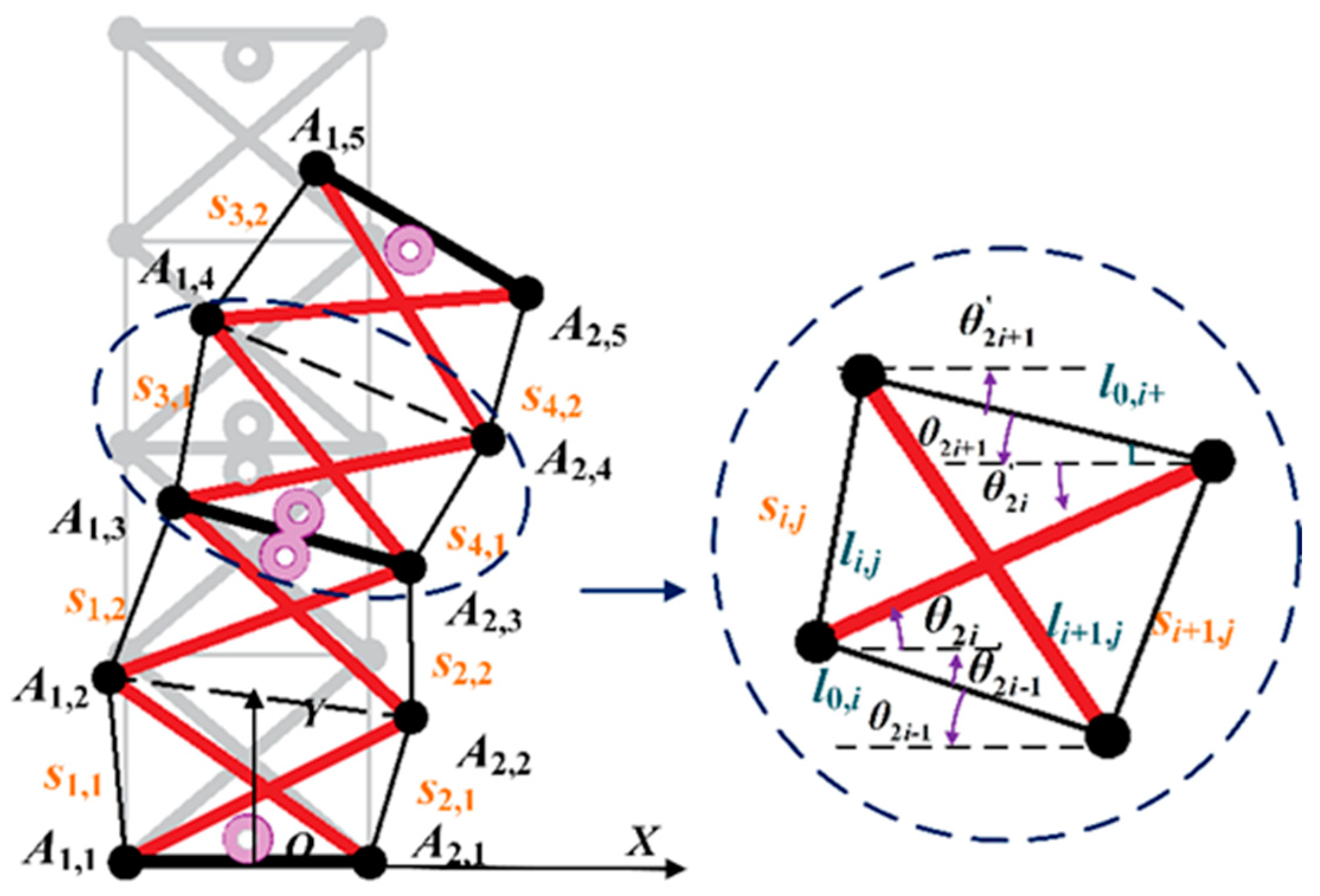
Since our tensegrity jumping robot has a symmetrical layout, we can simplify the configuration diagram of our robot as shown in Figure 3. The dimensions of the mechanism of the tensegrity jumping robot remain unchanged after the equivalence. At the same time, the mass and the moment of inertia of the mechanism after the equivalence show a superposition property, i.e., their values are equal to the sum of the corresponding parameters before the equivalence. We establish the plane rectangular coordinate system O-XY in Figure 3 and set the midpoint of the rack A1,1A2,1 as the origin. The X-axis is horizontally to the right and the Y-axis is vertically up. The X-axis is horizontally to the right and the Y-axis is vertically up.
Given that the main masses of the tensegrity jumping robot are concentrated on the geometric centers of the racks L0,1(A1,1A2,1), L0,3(A1,3A2,3), and L0,5(A1,5A2,5), we focus the masses mainly on these three key components to simplify the model and to highlight the main influencing factors during the kinematic modeling. In addition, considering that the friction between the sliding rope and each node has a relatively small effect on the overall motion, we chose to ignore this factor during the modeling process to ensure the accuracy and computational efficiency of the model.
It is worth noting that due to the uniqueness of the structural design of the tensegrity jumping robot, the magnitude of the axial force exerted on each portion of the broken ropes at nodes A1,2, A1,4, A2,2, and A2,4 remains the same. This property makes the lengths of the ropes on both sides of the above nodes equal, thus simplifying our analytical process. Thus, the equal lengths of the ropes on both sides of the above node can be expressed by us as
s k , 1 = s k , 2 = s k , 1 0 + φ k R k 4 , k = 1 ~ 4
where si,j (i = 1~4 and j = 1~2) are the lengths between the critical points of the two phases, respectively, and s i , j 0 is the length of the sliding rope in the initial state. φi (i = 1~4) denotes the input angles of the four main drive motors and Ri (i = 1~4) denotes the radii of the four winding disks of the tensegrity jumping robot.
Also from the geometric relations, we obtain
s 1 , 1 + l 0 , 1 + l 2 , 1 = 0 s 2 , 1 + l 0 , 1 + l 1 , 1 = 0 s 1 , 1 + l 1 , 1 + l 0 , 2 = 0
s 4 , 1 + l 0 , 5 + l 4 , 2 = 0 s 3 , 1 + l 0 , 5 + l 3 , 2 = 0 s 4 , 2 + l 3 , 2 + l 0 , 4 = 0
According to Equations (2) and (3) we can obtain
θ 1 , i = arccos l 1 , 1 2 i 2 s 1 , 1 4 2 I + l 0 , 1 2 s 2 , 1 2 i 2 l 2 , 1 4 2 i 2 l 1 , 1 i 1 s 1 , 1 2 i l 0 , 1 θ 2 , i = arccos s 4 , 2 2 i 2 l 3 , 2 4 2 i + l 0 , 5 2 l 4 , 2 2 i 2 s 3 , 2 4 2 i 2 s 4 , 2 i 1 l 3 , 2 2 i l 0 , 5 i = 1 , 2
θ 3 , i = θ 1 , i θ 2 , i i = 1 , 2
where θ1,1 represents the angle between rod A1,2A1,1 and rod A1,1A2,2, θ1,2 represents the angle between rod A1,2A1,1 and rod A1,1A2,2, θ2,1 represents the angle between rod A2,4A2,5 and rod A2,5A1,5, and θ2,2 represents the angle between rod A1,4A2,5 and rod A2,5A1,5. θ3,1 is the angle between rod A1,2A1,1 and rod A1,1A2,2 and θ3,2 is the angle between rod A1,4A2,5 and rod A2,5A2,4. Therefore, according to the cosine theorem, the lengths l0,2 and l0,4 of the racks L0,2 and L0,4 can be expressed, respectively, as
l 0 , 2 = l 1 , 1 2 + s 1 , 1 2 2 l 1 , 1 s 1 , 1 cos θ 3 , 1 1 2
l 0 , 4 = s 4 , 2 2 + l 3 , 2 2 2 s 4 , 2 l 3 , 2 cos θ 3 , 2 1 2
As shown in Figure 3, the structure formed by the rods, springs, and four sections of ropes in the tensegrity is taken as the basic unit for kinematic analysis and the several closed loops contained in it can be expressed as follows
l 1 , 1 + l 0 , i + s 3 i , 1 = 0 l 1 , 2 + l 0 , i + 1 + s 3 i , 2 = 0 l 3 , 1 + l 0 , i + 2 + s 5 i , 1 = 0 l 3 , 2 + l 0 , i + 3 + s 5 i , 2 = 0 i = 1 , 2
According to Formula (8) and the geometric relationship in the figure, we can obtain the angle of each rod and spring with the X-axis
θ i = arccos l 1 , 1 2 + l 0 , i 2 s 3 i , 1 2 2 l 1 , 1 l 0 , i θ i 1 θ i + 2 = arccos l 1 , 2 2 + l 0 , i + 1 2 s 3 i , 2 2 2 l 1 , 2 l 0 , i + 1 θ i + 1 θ i + 4 = arccos l 3 , 1 2 + l 0 , i + 2 2 s 5 i , 1 2 2 l 3 , 1 l 0 , i + 2 θ i + 3 θ i + 6 = arccos l 3 , 2 2 + l 0 , i + 3 2 s 5 i , 2 2 2 l 3 , 2 l 0 , i + 3 θ i + 5 i = 1 , 2
where we let θ 1 = 0. From the geometric relation, we know that θi = θ i (i = 1~7). From this, we know that the center of mass positions X0,3, Y0,3, and X0,5, Y0,5 of rack L0,3, and rack L0,5, respectively, can be denoted as
Y 0 , 3 = l 1 · η 1 X 0 , 3 = 0.5 l 0 , 1 + l 1 · η 2
Y 0 , 5 = l 1 · η 1 + l 2 · η 3 X 0 , 5 = 0.5 l 0 , 1 + l 1 · η 2 + l 2 · η 4
where the expressions of l1, l2, η1, η2, η3, and η4 can be found in Appendix A.
Since a functional relationship between the motor’s rotational angle φi (i = 1, 2, 3, 4) exists, at the time t, we can learn that the velocities at the center-of-mass positions of racks L0,3 and racks L0,5 can be expressed as
v Y 0 , 3 = l 1 · Q 1 v X 0 , 3 = l 1 · P 1
v Y 0 , 5 = l 1 · Q 1 + l 2 · Q 2 v X 0 , 5 = l 1 · P 1 + l 2 · P 2
where the expressions of Q1, Q2, P1, and P2 can be found in Appendix A.
The acceleration to the center of mass position of rack L0,3 and rack L0,5 at the same time can be expressed as
a Y 0 , 3 = l 1 · Q 3 + H 1 a X 0 , 3 = l 1 · P 3 + I 1
a Y 0 , 5 = l 1 · Q 3 + H 1 + l 2 · Q 4 + H 2 a X 0 , 5 = l 1 · P 3 + I 1 + l 1 · P 4 + I 2
where the expressions of Q3, Q4, P3, P4, H1, H2, I1, and I2 can be found in Appendix A. And the length variations Δl0,2 and Δl0,4 of rack L0,2 and rack L0,4 can be expressed as
Δ l 0 , 2 i = l 0 , 2 i l 0 , 2 i 0 i = 1 , 2
where l 0 , 2 0 denotes the original length of spring L0,2 and l 0 , 4 0 denotes the original length of spring L0,4.
In our study, we conducted in-depth kinematic analysis to examine the mathematical relationship between the input angle φi (i = 1, 2, 3, 4) of the four drive motors of the tensioning mobile robot and the position, velocity, and acceleration of the center of mass of the key rods. The establishment of this mathematical model not only provides us with the possibility to accurately describe the robot attitude but also provides an important basis for the subsequent motion plan and control strategy formulation of the robot. Through this model, we are able to understand the motion characteristics of the robot under different input angles more deeply, predict its trajectory and velocity changes, and then optimize its performance and improve its work efficiency.
On the basis of robot kinematic modeling, we further carried out the dynamic modeling of the tensegrity jumping robot. The construction of this model aims to deeply study the dynamic characteristic parameters such as kinetic energy and potential energy of the robot in the process of movement. From Equations (12) and (13), we can learn that the total kinetic energy E of the system during the jumping process is
E = 0.5 i = 1 2 m 0 , 2 i + 1 v Y 0 , 2 i + 1 2 + v X 0 , 2 i + 1 2
The potential energy of the system, on the other hand, can be expressed as
U = i = 1 2 m 0 , 2 i + 1 g Y 0 , 2 i + 1 + 0.5 k 2 i Δ l 0 , 2 i 2
where U represents the total potential energy of the system, k2 denotes the stiffness of the spring L0,2, and k4 denotes the stiffness of the spring L0,4. Thus, the tensegrity jumping robot Lagrangian quantity can be expressed as
L = i = 1 2 0.5 m 0 , 2 i + 1 v Y 0 , 2 i + 1 2 + v X 0 , 2 i + 1 2 m 0 , 2 i + 1 g Y 0 , 2 i + 1 0.5 k 2 i Δ l 2 i 2 = m = 1 4 n = 1 4 f m , n φ ˙ m φ ˙ n 0.5 i = 1 2 k 2 i Δ l 2 i 2 i = 1 2 m 0 , 2 i + 1 g Y 0 , 2 i + 1
where the expression of fi,j can be found in Appendix A.
Then, its Lagrangian equation can be expressed as
d d t L φ ˙ i L φ i = j = 1 4 d f j , i d t φ ¨ i + d f i , i d t φ ¨ i m = 1 4 n = 1 4 f m , n φ i φ ˙ m φ ˙ n + m = 1 2 k 2 m Δ l 2 m φ i + n = 1 2 m 0 , 2 n + 1 g Y 0 , 2 n + 1 φ i = 0 i = 1 ~ 4
where φi ∈ [0, φe] and φe is the limit driving angle of the robot. In particular, we can express it as
φ e = f e X e , Y e
where Xe and Ye are the coordinates of the center of mass of L0,5 when the robot moves to the limit position. We can define
Y e 2 + X e 2 = 1 4 i = 1 4 j = 1 2 s i , j 2 2

3.1.2. Dynamic Modeling of Two Modules’ Step-Up Jump

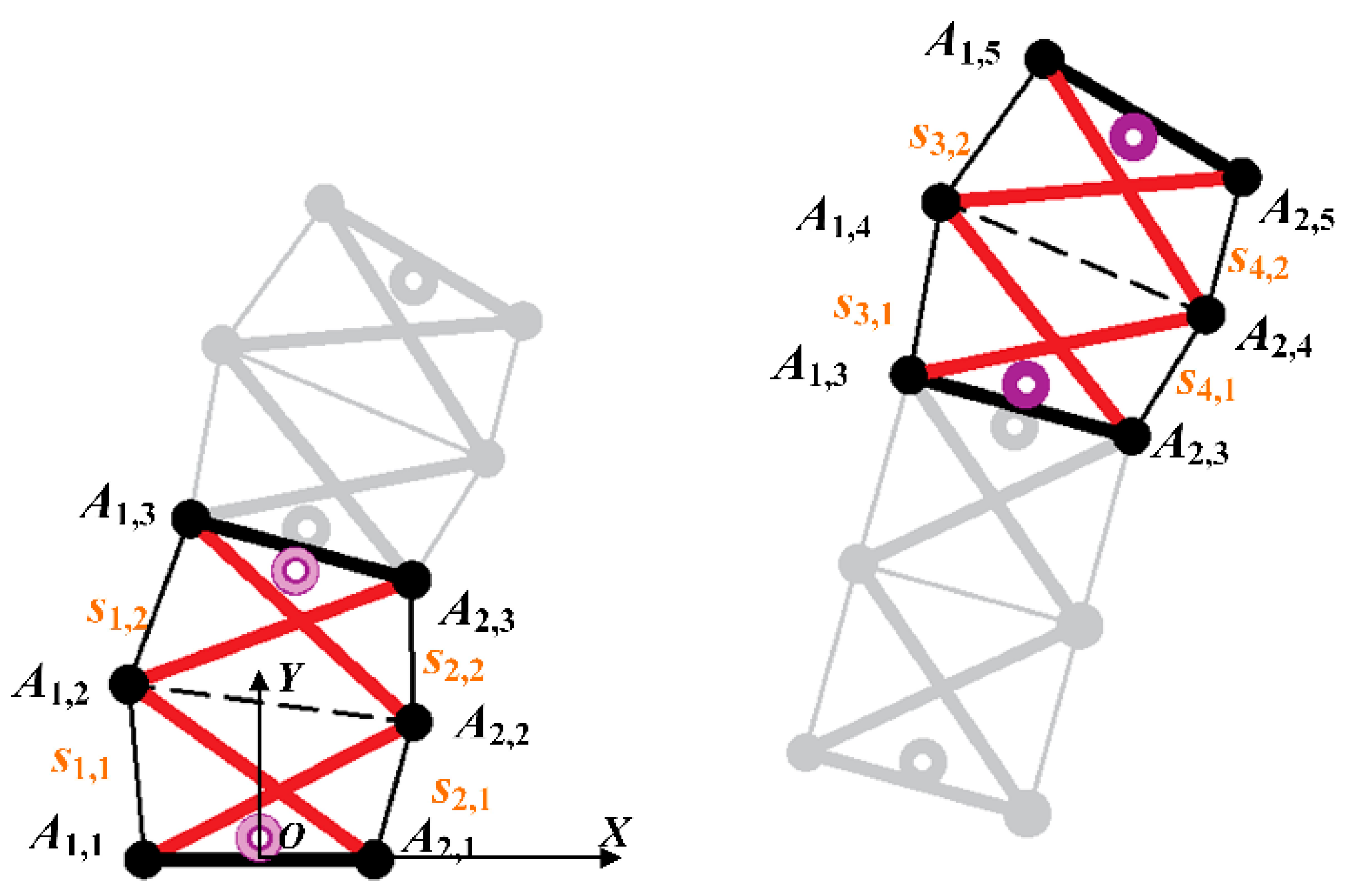
During the step-up process of the tensegrity jumping robot, we choose the module below the robot to release energy in priority, so in the process of releasing energy in the first module, we can accordingly establish the corresponding planar Cartesian coordinate system the Planar Cartesian Coordinate System O-XY and set the mid-point of the rod A1,1 A2,1 as the origin. The X-axis is horizontally to the right and the Y-axis is vertically up, as shown in Figure 4.
At this time, θi (i = 1~4) can be seen in Equation (9), the center of mass position Y 0 , 3 0 , X 0 , 3 0 of L0,3 can be seen in Equation (10) and the velocities v Y 0 , 3 0 and v X 0 , 3 0 and accelerations a Y 0 , 3 0 and a X 0 , 3 0 of the center of mass position of the rack L0,3 can be seen in (12) and (14). After the time Δt has elapsed, the tensegrity jumping robot makes a parabolic motion in the air. At this time, we can obtain (i = 5~8) (refer to Equation (9)). At this time, the velocity of the robot can be expressed as
v Y 0 , 3 = v Y 0 , 3 0 + a Y 0 , 3 0 Δ t v X 0 , 3 = v X 0 , 3 0 + a X 0 , 3 0 Δ t
The displacement of the robot during this time period can be represented as
x Y 0 , 3 = v Y 0 , 3 0 t Δ + 0.5 a Y 0 , 3 0 Δ t 2 X X 0 , 3 = v X 0 , 3 0 t Δ + 0.5 a X 0 , 3 0 Δ t 2
At this point, the center of mass position of the rack L0,3 can be represented as
Y 0 , 3 = Y 0 , 3 0 + x Y 0 , 3 X 0 , 3 = X 0 , 3 0 + x X 0 , 3
At this point, the center of mass position of the rack L0,1 can be represented as
Y 0 , 1 = X 0 , 3 2 Y 0 , 3 + Y 0 , 3 3 Y 0 , 3 2 s a v 2 X 0 , 3 2 + Y 0 , 3 2 X 0 , 3 2 + Y 0 , 3 2 X 0 , 1 = Y 0 , 3 2 X 0 , 3 + X 0 , 3 3 X 0 , 3 2 s a v 2 X 0 , 3 2 + Y 0 , 3 2 X 0 , 3 2 + Y 0 , 3 2
where the expressions of sav can be found in Appendix A.
Then, at this point, it is known that the velocity at the center of mass position of rack L0,1 is the same as that of L0,3. The center of mass position of rack L0,5 can refer to Equation (11). The velocity at the center of mass position of L0,5 at this time can be referred to as Equation (13). The kinetic energy and potential energy of the robot are
E = 1 2 i = 1 3 m 0 , i v Y 0 , i 2 + v X 0 , i 2
U = k 4 Δ l 4 2 2 + k = 1 3 m 0 , 2 i 1 g Y 0 , 2 i 1
At this point, it is known that the Lagrangian quantity is
L = m = 1 4 n = 1 4 z m , n φ ˙ m φ ˙ n k 4 l 4 2 2 i = 1 3 m 0 , 2 i 1 g Y 0 , 2 i 1
where the expressions of zi,j can be found in Appendix A.
Thus, the Lagrange equation is
d d t L φ ˙ i L φ i = j = 1 4 d z j , i d t φ ¨ i + d z i , i d t φ ¨ i m = 1 4 n = 1 4 z m , n φ i φ ˙ m φ ˙ n + k 4 Δ l 4 φ i + n = 1 3 m 0 , 2 n 1 g Y 0 , 2 n 1 φ i = 0 i = 1 ~ 4
where φi ∈ [0, φe] and the expression of φe are referred to in Equations (21) and (22).

3.2. Performance Analysis

3.2.1. Performance Analysis of Simultaneous Jumps

Based on the known Lagrangian equations, we can derive the jump case using programming tools. With a stiffness of the elastic cable of [0, 40] N/mm and an initial tilt angle of the robot body of [0, 18]°, we obtain Figure 5.
According to Figure 5, we can conclude that under the same conditions, the jump height of the robot increases significantly with the increase in stiffness. In particular, when the stiffness is 40 N/mm and the inclination angle is 0, the jump height of the robot is 679.42 mm. Meanwhile, the lateral jump distance of the robot increases with the increase in stiffness. When the stiffness is 40 N/mm and the inclination angle is 18°, the jump distance of the robot is 59.75 mm. This is because the greater the stiffness of elastic cables of the robot, the greater the potential energy stored by the robot, which enables the robot a higher jumping performance. Also, as the tilt angle of the robot increases, the jump height of the robot decreases but the lateral jump distance increases. This is due to the fact that the larger the tilt angle, the more kinetic energy the robot shares in the transverse direction and the less kinetic energy in the longitudinal direction. In this case, we select the jumping schematic of the robot with a stiffness of 16 N/mm and a tilt angle of 18°, as shown in the right section of Figure 5, where the robot’s jumping height is 80.84 mm and the jumping distance is 3.83 mm. Therefore, to enhance the jumping performance of the robot effectively, it is advisable to moderately augment the stiffness of the elastic cables.

3.2.2. Performance Analysis of A Step-Up Jump

Using the same method, it is possible to obtain the jumping performance of the step-up jumping process of the robot, as shown in Figure 6. We analyzed the jump performance of the robot step-up release after four Δt time periods. In particular, the change ranges of stiffness of the elastic cable and the initial tilt angle, which are consistent with those observed during the simultaneous jumping process of the robot, are significant factors.
According to Figure 6, we can see that the robot can achieve better jumping performance if the release timing is chosen appropriately. In particular, the robot can achieve greater energy utilization by releasing the energy of the second module when the kinetic energy in the vertical direction is about to be zero, following the release of the first module, specifically during the Δt3 period depicted in Figure 6. At this time, we obtained the maximum jump height of 782.14 mm and the jump distance of 85.26 mm, which is better than the performance of simultaneous jumping of the two modules (Figure 6). This is due to the fact that step-up jumping can improve the efficiency of energy utilization and reduce energy loss. Therefore, for a modular jumping robot, step-up jumping of each module can enable the robot a better jumping performance.

3.3. Simulations Analysis

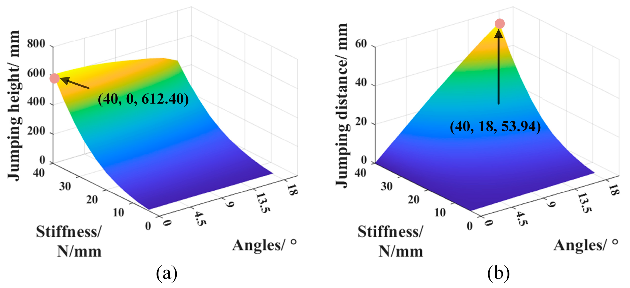
In this section, dynamic simulations of the robot are carried out to verify the feasibility of robot design and performance analysis. The simulation of simultaneous jumping performance for different parameter cases was tested, as shown in Figure 7.
The maximum jump height obtained from our simulation is 612.40 mm and the maximum jump distance is 53.94 mm. The comparison shows that the jumping performance of the robot increases as the stiffness of the spring increases for the same case. This is due to the fact that the higher the stiffness, the more energy the robot stores. The higher the tilt angle of the robot, the jumping performance of the robot decreases but the distance traveled to the side increases.
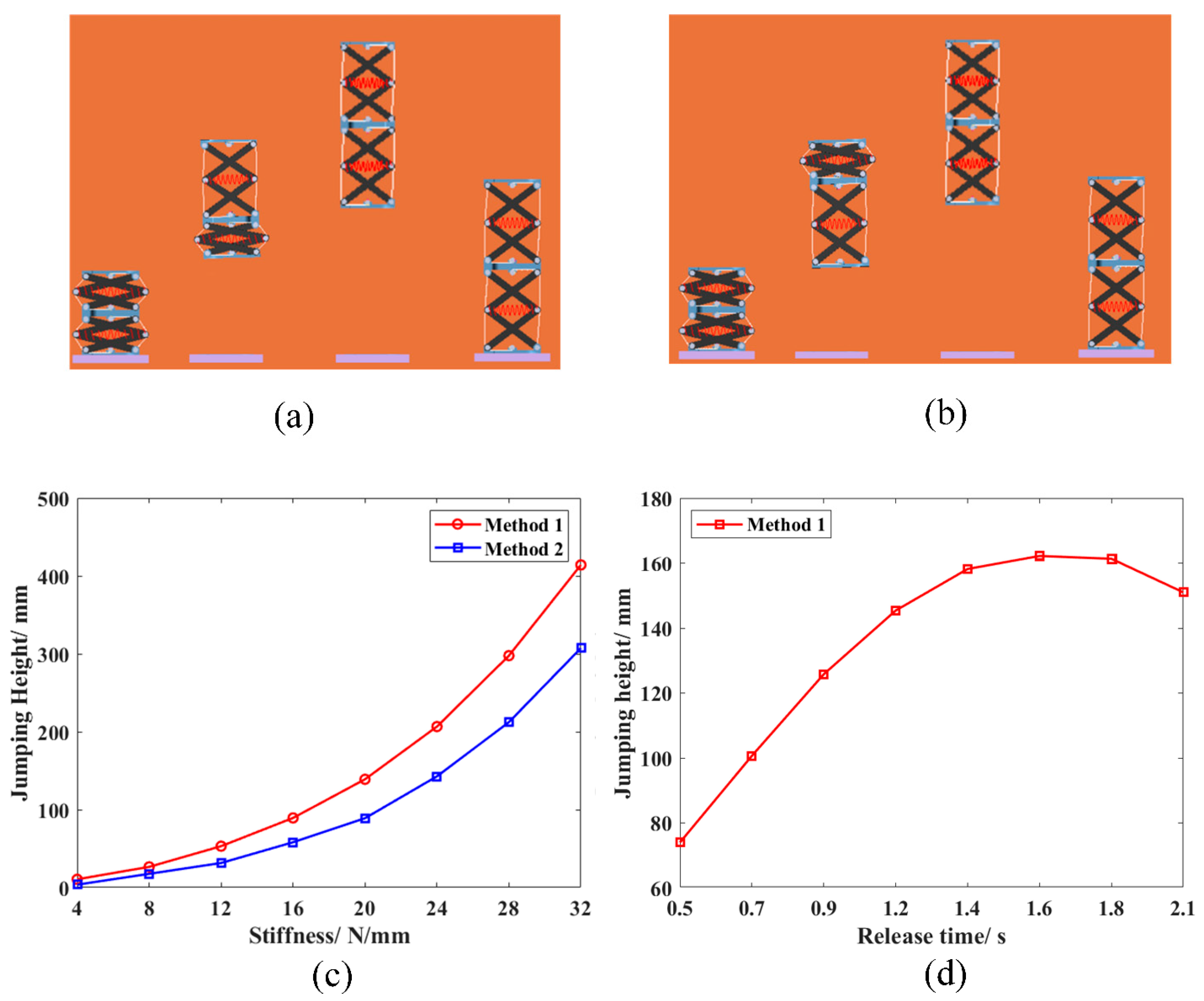
During the step-up jumping performed by the tensegrity jumping robot, it is theoretically known that differing sequences of energy release and the choice of specific energy release moments will affect the jumping results of the robot. We tested several groups of jumping performance of energy release methods with different stiffness cases. The two jumping methods in each group had the same conditions except for the jumping mode. As shown in Figure 8, the first way is to release the energy of the module below the robot first and then release the energy of the module above the robot after the robot is airborne; as shown in Figure 8, the second way is the opposite. Taking the release time of Δt3 as an example, the simulation results are shown in Figure 8. It can be found that the energy utilization of the first way is better than the second one. When the stiffness of elastic cable is 28 N/m, the jumping height of the two ways are 276.15 mm and 297.36 mm, respectively.
Secondly, the choice of energy release moment in the second module also affects the robot’s jump result parameters. As shown in Figure 8, taking the first way for releasing the energy as an example, eight moments are selected to analyze the efficiency of energy release under different moment choices. We can see that the robot energy utilization efficiency shows a trend of increasing and then decreasing as time moves backward. When the release time is 0.5 s, the jumping height is 73.15 mm, and when the release time is 2.1 s, the jumping height is 150.76 mm.
On the basis of the above analysis, we tested the jumping height and diagonal jumping distance of the tensegrity jumping robot when the robot is tilted at different angles for two-module step-up jumping within a certain stiffness range. Taking the release time of 1.6s and the first way for releasing the energy as an example, the jumping performance of the robot is shown in Figure 9.
The maximum jump height obtained from our simulation is 712.16 mm and the maximum jump distance is 63.67 mm. According to Figure 9, we can see that when other conditions are the same, the larger the stiffness is, the robot’s jumping height and jumping distance will increase. The larger the tilt angle is, the robot’s jumping performance in the vertical direction will be reduced accordingly and the jumping distance in the horizontal direction will be increased.

4. Experiment Verification

4.1. Prototype of the Robot

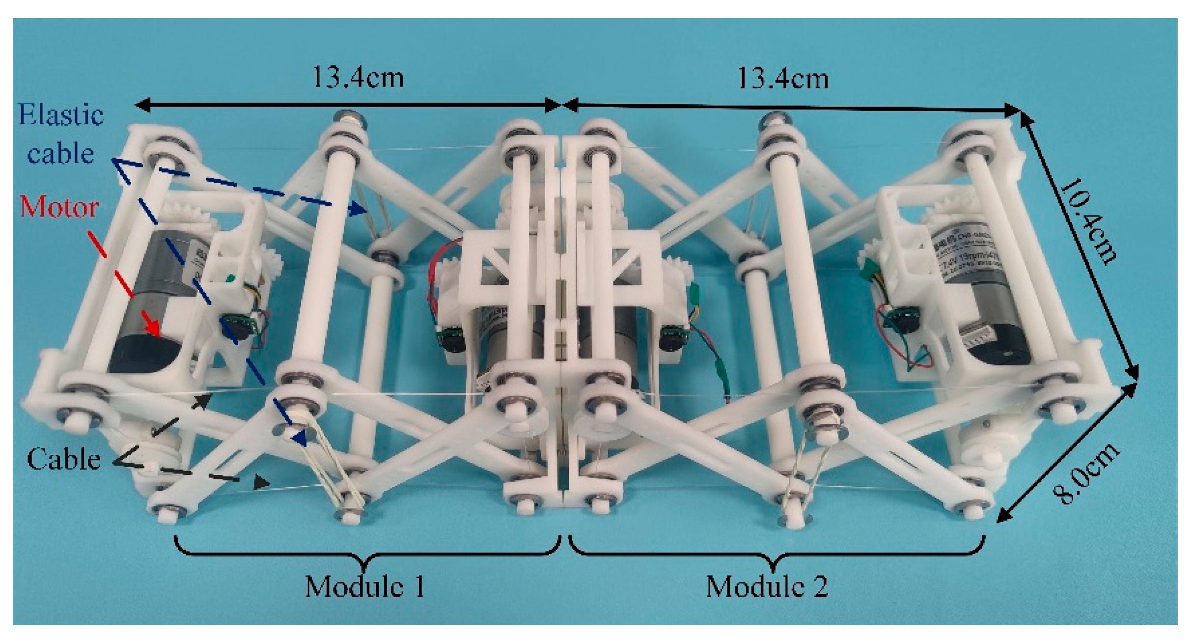
In order to validate the proposed kinematic modeling approach, we built a two-module robot prototype for experimentation, as shown in Figure 10. The driving laws of the motors and the values of all parameters of the prototype, including the stiffness coefficients and the original lengths of the elastic cables, agree with the theoretical optimization results. Each module consists of two elastic storage mechanisms and four elastic cables. Each module consists of two elastic storage mechanisms and four elastic cables. The robot’s individual module measures 8.0 cm × 10.4 cm × 13.4 cm and weighs 470 g. The robot is designed for use in a variety of applications. The main structure of the robot is made of 3D-printed photosensitive resin material. The control system of each module consists of a controller (Model: STM32F103ZET6) and two motor drivers (Model: L298N), two geared motors with large reduction ratios (Model: 25GA310), and two small geared motors (Model: GM12-N20).
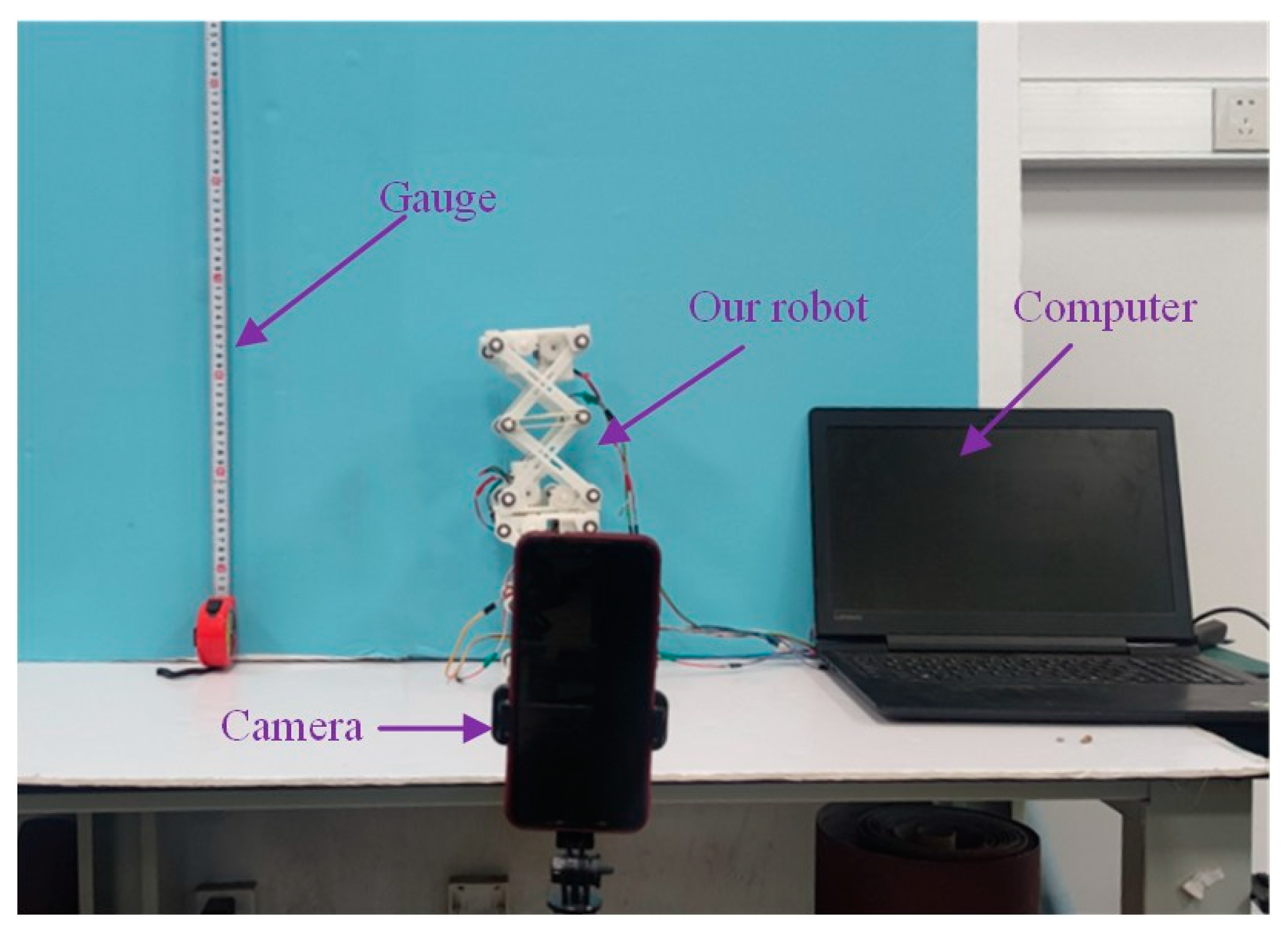
In order to ensure the smooth running of the experiment and to obtain accurate and reliable data, it is crucial to build an appropriate experimental environment. We built the experimental environment as shown in Figure 11; the specific parameters of the device camera are the customized 48-megapixel sensor OV48C from Howell Technologies as the main camera (f/1.9, 1/1.32”). Among other things, it is important to make sure that the lab bench stays level and is not tilted. Before the experiment is formally carried out, the robot model, power supply, measurement equipment, and so on should be thoroughly checked to avoid accidents during the experiment.

4.2. Experimental Results

This experiment aims to evaluate the performance of the jumping robot in a real environment and compare it with the simulation results. The objective is to verify the accuracy of the theoretical model and provide practical data support for further optimization of the robot. By analyzing the role of stiffness, it provides data support for design optimization and, by comparing the simulation results under different stiffness, it provides a comprehensive understanding of the role of stiffness in jumping robots and guides the actual design and control optimization.
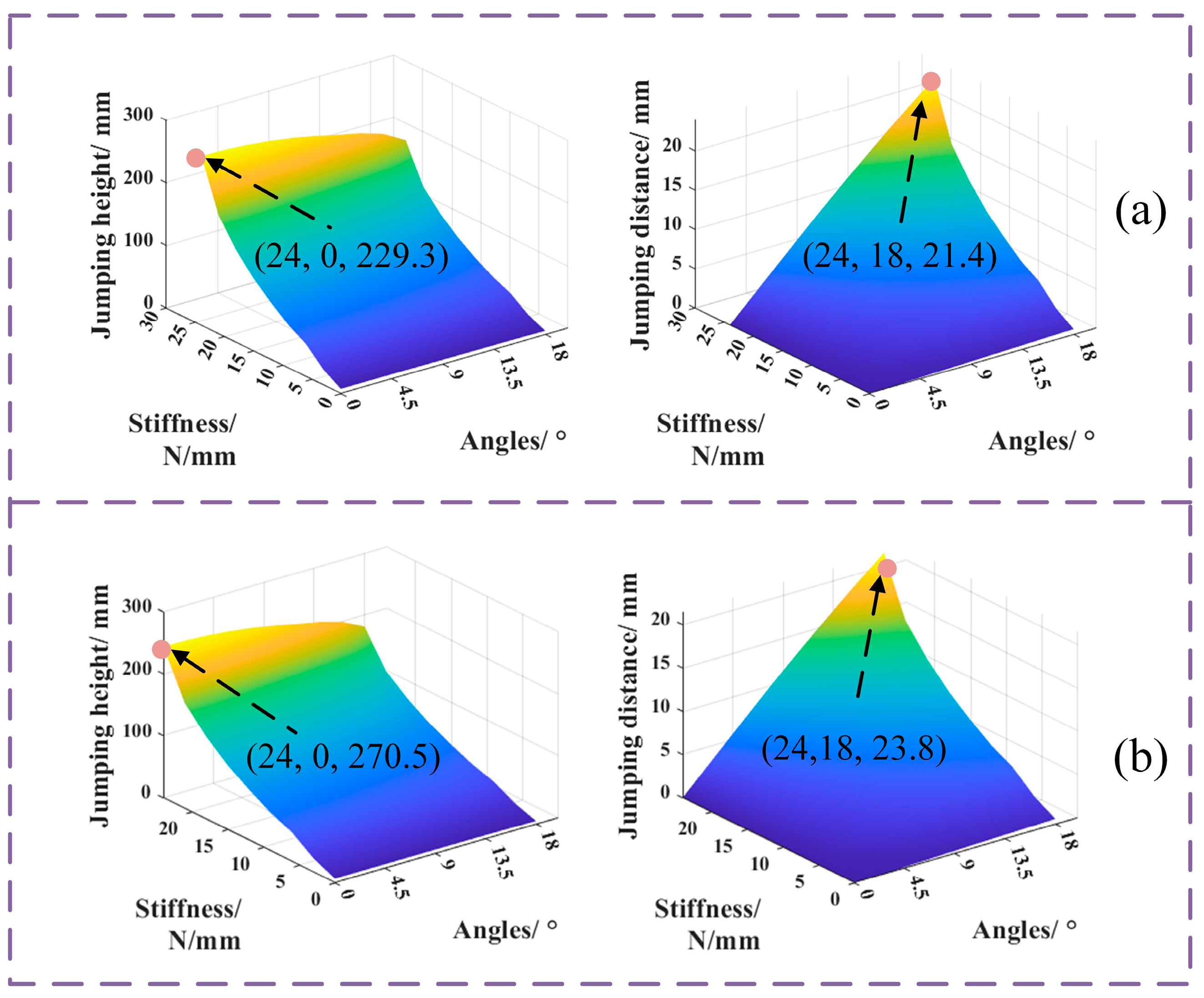
We tested the jumping performance of the prototype for stiffnesses ranging from 0 to 24 N/mm and tilt angles ranging from 0 to 18°, as shown in Figure 12 and Figure 13. We summarized the experimental data we obtained, as shown in Figure 14. When the robots were released at the same time, we experimentally measured a maximum jump height of 229.32 mm and a maximum jump distance of 21.42 mm. When the step-ups were released, we experimentally measured a maximum jump height of 270.59 mm and a maximum jump distance of 23.86 mm. We choose the position Δt3 above to release the energy of the second module. Moreover, it can be seen from the experimental results (Figure 12 and Figure 13) that the robot can achieve a stable jumping process on the two occasions, which benefits from the stable tensegrity structure.
For the experiments with simultaneous jumping, the maximum error between our measured data and the simulated data is 9.1%, while the maximum difference between the experimental data and the simulated data for step-up jumping is 13.2%. The overall experimental results match the results of the simulation. A better jumping effect can be obtained by increasing the stiffness and a larger lateral travel distance can be obtained by tilting the fuselage. At maximum, the jumping performance of step-up jumping was approximately 24% higher than the jumping height of simultaneous jumping. A higher energy utilization efficiency can be obtained by step-up jumping and a higher jumping distance can be obtained under the same conditions.

5. Conclusions

Most of the existing jumping robots cannot achieve stable jumping and they also have low energy utilization efficiency, which limits their practical applications. To this end, a tensegrity-based jumping robot is proposed in this work, which is composed of two identical modules. Dynamic models of the robot are established to overcome the abovementioned problems. Simulations and experiments are conducted to verify the rationality of the proposed robot.
(1)
The design process of the tensegrity-based jumping robot is elaborated in the context and the jumping mechanism of the robot is analyzed;
(2)
Dynamic models of the robot are established, which include two modules’ simultaneous jumping and step-up jumping processes. Performance analysis for different jumping processes is conducted and the interrelation between parameters and performance is established;
(3)
The simulation and experiment results show that our jumping robot can achieve a stable jumping process and the step-up jumping of each module of the prototype can have higher energy efficiency than that of simultaneous jumping of each module, which enables the robot a better jumping performance.
In the field of jumping robot design, a general rule exists: the smaller and lighter the size of the robot and the higher the output torque of the motors, the better its jumping performance tends to be. However, the robots we have designed so far are limited by the performance of the motors, resulting in their relatively large size and mass. This undoubtedly affects the jumping performance of the robot to a certain extent, making it difficult to reach the desired level. In order to further improve the jumping performance of the robot, we plan to look for motors with smaller sizes and higher output torque in our future research. Such motors will allow us to design a more compact robot with better jumping ability.
A further extension to this work could include the design and control of a spatial jumping robot based on the spatial tensegrity structure, such as a 3-strut and 9-cable structure or a 4-strut and 12-cable structure, to endow the jumping robot with more redundant jumping patterns, to make it possible to tilt jump in multiple directions. In addition to this, we subsequently propose to build at least three modules of jumping robots to obtain a better jumping effect.

Author Contributions

Conceptualization, Q.Y., B.L. and G.T.; methodology, G.T. and Q.Y.; software, G.T.; validation, G.T. and Q.Y.; investigation, G.T. and Q.Y.; writing—original draft preparation, G.T.; writing—review and editing, G.T., Q.Y. and B.L.; funding acquisition, B.L. All authors have read and agreed to the published version of the manuscript.

Funding

This research was funded by the National Natural Science Foundation of China, grant number 52275028.

Institutional Review Board Statement

Not applicable.

Informed Consent Statement

Not applicable.

Data Availability Statement

The original contributions presented in the study are included in the article, further inquiries can be directed to the corresponding author.

Conflicts of Interest

The authors declare no conflicts of interest.

Appendix A

A i = X 0 , 1 φ i / φ ˙ i B i = X 0 , 1 φ i / φ ˙ i C i = X 0 , 3 φ i / φ ˙ i D i = Y 0 , 3 φ i / φ ˙ i E i = X 0 , 5 φ i / φ ˙ i F i = Y 0 , 5 φ i / φ ˙ i i = 1 ~ 4
Q i , j = sin θ i d d t θ i j
P i , j = cos θ i d d t θ i j
H i , j = sin θ i d 2 d t 2 θ i j
I i , j = cos θ i d 2 d t 2 θ i j
f i , j = m 0 , 3 2 ( C i C j + D i D j ) + m 0 , 5 2 ( E i E j + F i F j )
z i , j = m 0 , 1 2 ( A i A j + B i B j ) m 0 , 3 2 ( C i C j + D i D j ) + m 0 , 5 2 ( E i E j + F i F j )
s a v = s 1 , 1 0 + s 1 , 2 0 + s 2 , 1 0 + s 2 , 2 0 2
l 1 = l 1 , 1 l 0 , 2 l 1 , 2 0.5 l 0 , 3 T
l 2 = 0.5 l 0 , 3 l 3 , 1 l 0 , 4 l 3 , 2 0.5 l 0 , 5 T
η 1 = sin θ 1 sin θ 2 sin θ 3 sin θ 4
η 2 = cos θ 1 cos θ 2 cos θ 3 cos θ 4
η 3 = sin θ 4 sin θ 5 sin θ 6 sin θ 7 sin θ 8
η 4 = cos θ 4 cos θ 5 cos θ 6 cos θ 7 cos θ 8
Q 1 = Q 1 , 1 Q 2 , 1 Q 3 , 1 0.5 Q 4 , 1
Q 2 = 0.5 Q 4 , 1 Q 5 , 1 Q 6 , 1 Q 7 , 1 0.5 Q 8 , 1
Q 3 = Q 1 , 2 Q 2 , 2 Q 3 , 2 Q 4 , 2
Q 4 = Q 4 , 2 Q 5 , 2 Q 6 , 2 Q 7 , 2 Q 8 , 2
P 1 = P 1 , 1 P 2 , 1 P 3 , 1 0.5 P 4 , 1
P 2 = 0.5 P 4 , 1 P 5 , 1 P 6 , 1 P 7 , 1 0.5 P 8 , 1
P 3 = P 1 , 2 P 2 , 2 P 3 , 2 P 4 , 2
P 4 = P 4 , 2 P 5 , 2 P 6 , 2 P 7 , 2 Q 8 , 2
H 1 = H 1 , 1 H 2 , 1 H 3 , 1 H 4 , 1
H 2 = P 4 , 2 P 5 , 1 , 2 P 6 , 1 , 2 P 7 , 1 , 2 P 8 , 1 , 2
I 1 = I 1 , 1 I 2 , 1 I 3 , 1 I 4 , 1
I 2 = I 4 , 1 I 5 , 1 I 6 , 1 I 7 , 1 I 8 , 1

References

  1. Elena, G.; Jimenez, M.A.; De Santos, P.G.; Armada, M. The Evolution of Robotics Research—From Industrial Robotics to Field and Service Robotics. IEEE Robot. Autom. Mag. 2007, 14, 90–103. [Google Scholar]
  2. Sun, T.; Zhai, Y.; Song, Y.; Zhang, J. Kinematic Calibration of a 3-Dof Rotational Parallel Manipulator Using Laser Tracker. Robot. Comput.-Integr. Manuf. 2016, 41, 78–91. [Google Scholar] [CrossRef]
  3. Sun, T.; Yang, S.-F.; Huang, T.; Dai, J.S. A Finite and Instantaneous Screw Based Approach for Topology Design and Kinematic Analysis of 5-Axis Parallel Kinematic Machines. Chin. J. Mech. Eng. 2018, 31, 44. [Google Scholar] [CrossRef]
  4. Ma, T.; Xu, X.; Chai, Z.; Wang, T.; Shen, X.; Sun, T. A Wearable Biofeedback Device for Monitoring Tibial Load During Partial Weight-Bearing Walking. IEEE Trans. Neural Syst. Rehabil. Eng. 2023, 31, 3428–3436. [Google Scholar] [CrossRef] [PubMed]
  5. Sun, T.; Liang, D.; Song, Y. Singular-Perturbation-Based Nonlinear Hybrid Control of Redundant Parallel Robot. IEEE Trans. Ind. Electron. 2017, 65, 3326–3336. [Google Scholar] [CrossRef]
  6. Sun, T.; Xiang, X.; Su, W.; Wu, H.; Song, Y. A Transformable Wheel-Legged Mobile Robot: Design, Analysis and Experiment. Robot. Auton. Syst. 2017, 98, 30–41. [Google Scholar] [CrossRef]
  7. Chen, K.; Wang, M.; Huo, X.; Wang, P.; Sun, T. Topology and Dimension Synchronous Optimization Design of 5-Dof Parallel Robots for in-Situ Machining of Large-Scale Steel Components. Mech. Mach. Theory 2023, 179, 105105. [Google Scholar] [CrossRef]
  8. Sun, T.; Yang, S. An Approach to Formulate the Hessian Matrix for Dynamic Control of Parallel Robots. IEEE/ASME Trans. Mechatron. 2019, 24, 271–281. [Google Scholar] [CrossRef]
  9. Liu, C.; Song, Y.; Ma, X.; Sun, T. Accurate and Robust Registration Method for Computer-Assisted High Tibial Osteotomy Surgery. Int. J. Comput. Assist. Radiol. Surg. 2023, 18, 329–337. [Google Scholar] [CrossRef]
  10. Sun, T.; Huo, X. Type Synthesis of 1t2r Parallel Mechanisms with Parasitic Motions. Mech. Mach. Theory 2018, 128, 412–428. [Google Scholar] [CrossRef]
  11. Bruzzone, L.; Quaglia, G. Locomotion Systems for Ground Mobile Robots in Unstructured Environments. Mech. Sci. 2012, 3, 49–62. [Google Scholar] [CrossRef]
  12. Francisco, R.; Valero, F.; Llopis-Albert, C. A Review of Mobile Robots: Concepts, Methods, Theoretical Framework, and Applications. Int. J. Adv. Robot. Syst. 2019, 16, 1729881419839596. [Google Scholar]
  13. Li, J.; Liu, Y.; Yu, Z.; Guan, Y.; Zhao, Y.; Zhuang, Z.; Sun, T. Design, Analysis, and Experiment of a Wheel-Legged Mobile Robot. Appl. Sci. 2023, 13, 9936. [Google Scholar] [CrossRef]
  14. Yang, Q.; Liu, X.; Wang, P.; Song, Y.; Sun, T. Multi-Locomotion Transition of Tensegrity Mobile Robot under Different Terrains. Sci. China Technol. Sci. 2023, 67, 536–557. [Google Scholar] [CrossRef]
  15. Li, J.; Liu, Y.; Yu, Z.; Guan, Y.; Zhao, Y.; Zhuang, Z.; Sun, T. A Low-Energy Consumption Planning Method for Multi-Locomotion Wheel-Legged Mobile Robots. Machines 2024, 12, 98. [Google Scholar] [CrossRef]
  16. Aravind, S.; Schäfer, B.; Hirzinger, G. Robot Mobility Systems for Planetary Surface Exploration–State-of-the-Art and Future Outlook: A Literature Survey. Aerosp. Technol. Adv. 2010, 492, 189–208. [Google Scholar]
  17. Zhang, C.; Zou, W.; Ma, L.; Wang, Z. Biologically Inspired Jumping Robots: A Comprehensive Review. Robot. Auton. Syst. 2020, 124, 103362. [Google Scholar] [CrossRef]
  18. Gal, R. Insect-Inspired Jumping Robots: Challenges and Solutions to Jump Stability. Curr. Opin. Insect Sci. 2020, 42, 32–38. [Google Scholar]
  19. Zhang, Y.; Li, P.; Quan, J.; Li, L.; Zhang, G.; Zhou, D. Progress, Challenges, and Prospects of Soft Robotics for Space Applications. Adv. Intell. Syst. 2023, 5, 2200071. [Google Scholar] [CrossRef]
  20. Paolo, F.; Burdick, J. The Development of Hopping Capabilities for Small Robots. Auton. Robot. 2003, 14, 239–254. [Google Scholar]
  21. Yan, H.; Zhu, X.; Hou, Z.; Wang, W.; Zhang, Z. Design and Motion Modeling of a Small-Scale Lunar Jumping Robot. J. Shanghai Jiaotong Univ. 2023, in press. [Google Scholar]
  22. Yun, R.; Liu, Z.; Leng, J.; Huang, J.; Yan, X.; Qi, M. A Millimeter-Scale Multilocomotion Microrobot Capable of Controlled Crawling and Jumping. Soft Robot. 2024, 11, 361–370. [Google Scholar] [CrossRef] [PubMed]
  23. Wu, M. Robotics Applications in Natural Hazards. Highlights Sci. Eng. Technol. 2023, 43, 273–279. [Google Scholar] [CrossRef]
  24. Yin, Z.; Yang, Z.; Van De Panne, M.; Yin, K. Discovering Diverse Athletic Jumping Strategies. ACM Trans. Graph. (TOG) 2021, 40, 1–17. [Google Scholar] [CrossRef]
  25. Umberto, S.; Stefanini, C.; Dario, P. A Bioinspired Concept for High Efficiency Locomotion in Micro Robots: The Jumping Robot Grillo. In Proceedings of the 2006 IEEE International Conference on Robotics and Automation (ICRA), Orlando, FL, USA, 15–19 May 2006. [Google Scholar]
  26. Tibert, A.G.; Pellegrino, S. Review of Form-Finding Methods for Tensegrity Structures. Int. J. Space Struct. 2011, 26, 241–255. [Google Scholar] [CrossRef]
  27. Donato, R.; Donati, E.; Benelli, G.; Stefanini, C. A Review on Animal–Robot Interaction: From Bio-Hybrid Organisms to Mixed Societies. Biol. Cybern. 2019, 113, 201–225. [Google Scholar]
  28. Tur Mirats, J.M.; Juan, S.H. Tensegrity Frameworks: Dynamic Analysis Review and Open Problems. Mech. Mach. Theory 2009, 44, 1–18. [Google Scholar] [CrossRef]
  29. Yang, Q.; Yu, Z.; Liu, X.; Lian, B.; Sun, T. A Small-Scale Untethered Tensegrity Robot with High Velocity and Multi Locomotion Modes. IEEE Robot. Autom. Lett. 2023, 8, 7503–7510. [Google Scholar] [CrossRef]
  30. Yang, Q.; Liu, X.; Wang, P.; Song, Y.; Sun, T. A Multi-Locomotion Clustered Tensegrity Mobile Robot with Fewer Actuators. Robot. Auton. Syst. 2023, 168, 104504. [Google Scholar] [CrossRef]
  31. Hiroshi, F. Concept of Deployable Tensegrity Structures in Space Application. Int. J. Space Struct. 1992, 7, 143–1451. [Google Scholar]
  32. Skelton, R.E.; Helton, J.W.; Adhikari, R.; Pinaud, J.-P.; Chan, W. An Introduction to the Mechanics of Tensegrity Structures. In The Mechanical Systems Design Handbook; CRC Press: Boca Raton, FL, USA, 2017; pp. 315–388. [Google Scholar]
  33. Brian, S.; Choxi, H.; Salamon, A.; Drewes, P. Advancing Robotics: The Urban Challenge Effect. J. Aerosp. Comput. Inf. Commun. 2008, 5, 530–542. [Google Scholar]
  34. Hendrik, K.; Breitenstein, M.; Gehring, C.; Hutter, M. Scalability Analysis of Legged Robots for Space Exploration. In Proceedings of the Unlocking Imagination, Fostering Innovation and Strengthening Security: 68th International Astronautical Congress (IAC 2017), Adelaide, Australia, 25–29 September 2017. [Google Scholar]
  35. Wang, Y.; Du, X.; Zhang, H.; Zou, Q.; Law, J.; Yu, J. Amphibious Miniature Soft Jumping Robot with on-Demand in-Flight Maneuver. Adv. Sci. 2023, 10, 2207493. [Google Scholar] [CrossRef] [PubMed]
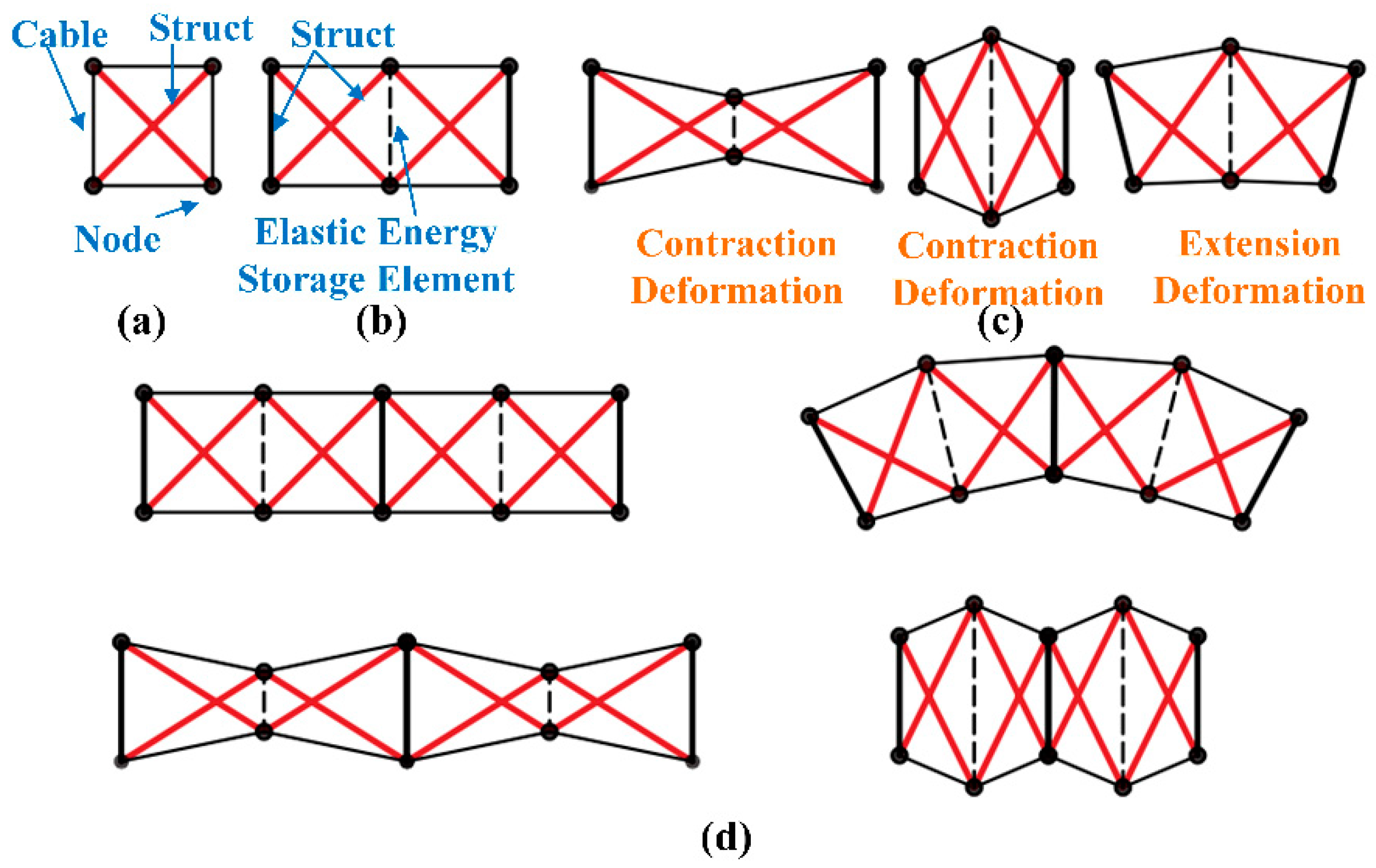
Figure 1. Tensegrity jumping robot design process. (a) 2-Strut 4-Cable. (b) Basic unit of tensegrity. (c) Tensegrity jumping robot basic unit. (d) Robot’s deformation forms.
Applsci 14 03947 g001
Figure 2. Three-dimensional models. (a) Initial state. (b) Compressed state. (c) Step-up state. (d) Trigger device.
Applsci 14 03947 g002
Figure 3. Diagram of the simultaneous jump.
Applsci 14 03947 g003
Figure 4. Diagram of the step-up jump.
Applsci 14 03947 g004
Figure 5. Dual module simultaneous jump. (a) Vertical jump height. (b) Horizontal jump distance. (c) Schematic diagram of jumps at 8° and 16 N/mm.
Applsci 14 03947 g005
Figure 6. Dual module step-up jump. (a) Jump height and jump distance at four moments. (b) Choice of jumping moments; (c) Schematic diagram of jumps at 8° and 16 N/mm.
Applsci 14 03947 g006
Figure 7. Simultaneous jump simulation. (a) Vertical jump height. (b) Horizontal jump distance.
Applsci 14 03947 g007
Figure 8. Release order and time. (a) Method 1; (b) Method 2; (c) Release order; (d) Release time.
Applsci 14 03947 g008
Figure 9. Step-up jumping simulation. (a) Vertical jump height. (b) Horizontal jump distance.
Applsci 14 03947 g009
Figure 10. Prototype of the robot with two modules.
Applsci 14 03947 g010
Figure 11. Environment of the experiment.
Applsci 14 03947 g011
Figure 12. Experiments with simultaneous jumping.
Applsci 14 03947 g012
Figure 13. Experiments with step-up jumping.
Applsci 14 03947 g013
Figure 14. Data from experiments. (a) Simultaneous jumping. (b) Step-up jumping.
Applsci 14 03947 g014
Disclaimer/Publisher’s Note: The statements, opinions and data contained in all publications are solely those of the individual author(s) and contributor(s) and not of MDPI and/or the editor(s). MDPI and/or the editor(s) disclaim responsibility for any injury to people or property resulting from any ideas, methods, instructions or products referred to in the content.