Autoencoder-Based DIFAR Sonobuoy Signal Transmission and Reception Method Incorporating Residual Vector Quantization and Compensation Module: Validation Through Air Channel Modeling

Abstract

This paper proposes a novel autoencoder-based neural network for compressing and reconstructing underwater acoustic signals collected by Directional Frequency Analysis and Recording sonobuoys. To improve both signal compression rates and reconstruction performance, we integrate Residual Vector Quantization and a Compensation Module into the decoding process to effectively compensate for quantization errors. Additionally, an unstructured pruning technique is applied to the encoder to minimize computational load and parameters, addressing the battery limitations of sonobuoys. Experimental results demonstrate that the proposed method reduces the data transmission size by approximately 31.25% compared to the conventional autoencoder-based method. Moreover, the spectral mean square errors are reduced by 60.58% for continuous wave signals and 55.25% for linear frequency modulation signals under realistic air channel simulations.

1. Introduction

Sonobuoys are disposable devices designed to detect and analyze underwater acoustic signals generated in the ocean. Primarily employed for military purposes, they are used to detect underwater targets, such as enemy submarines, and play a pivotal role in Anti-Submarine Warfare (ASW) [1]. Sonobuoys are typically employed in multi-static detection systems, where multiple sonobuoys operate collaboratively to enhance detection capabilities. In this setup, the transmitter and receiver are positioned separately, providing a wider detection range and improved operational confidentiality compared to monostatic configurations. Notably, the bistatic mode is a simplified version of multi-static detection, involving a single transmitter and receiver operating from separate locations, embodying the basic principles of multi-static systems [2].

This equipment comprises a buoy and an acoustic collection device. The acoustic collection device gathers acoustic signals generated underwater, and the collected signals are transmitted via the buoy to platforms such as Maritime Patrol Aircraft (MPA) [3]. The platform analyzes the received signals to detect and classify underwater targets. Figure 1. illustrates the underwater acoustic collection scenario in a bistatic environment using active and passive sonobuoys in ASW, where the collected acoustic signals are transmitted through wireless communication to the MPA.

During the wireless communication process, fading phenomena can occur during signal transmission due to factors such as reflection, refraction, diffraction, and scattering along the propagation path [4]. Fading refers to temporal fluctuations in signal strength and quality, which can adversely impact communication performance. In Figure 1, the schematic visualizes these fading phenomena by depicting a 2-Ray Propagation scenario encompassing both LOS and NLOS conditions.

Conventionally, acoustic signals collected by sonobuoys are typically transmitted via wireless communication by modulating the converted signals using Frequency Division Multiplexing (FDM) [5]. However, the FDM approach has several significant limitations. First, a large amount of data transmission is required because the entire acoustic signal is transmitted, which can lead to inefficient consumption of communication resources. Second, multiplexed signals can be relatively easily identified within the frequency band, presenting vulnerabilities in terms of information security [6]. Due to these limitations, relying solely on conventional FDM methods makes it difficult to ensure efficient and secure data transmission between sonobuoys and MPA. Therefore, the introduction of new data transmission methods is required.

In this regard, audio compression techniques can be an alternative and various techniques for audio compression have been explored for decades [7,8,9,10,11,12,13,14]. Traditional audio data compression techniques are broadly categorized into waveform codecs [7] and parametric codecs [8], each focusing on either high-fidelity reconstruction or low bit-rate efficiency. These codecs are designed through signal processing pipelines and meticulous engineering [9]. Recently, advancements in deep learning technologies have led to the introduction of neural network-based approaches in audio codecs, garnering attention for end-to-end codecs that learn complex patterns of input signals and enable high-quality signal reconstruction [9,10,11]. These codecs, referred to as neural codecs, extract key features of the signals and perform efficient compression and reconstruction, demonstrating outstanding performance across various types of audio. In particular, a prominent neural codec is SoundStream [9]. SoundStream employs a quantization technique known as Residual Vector Quantization (RVQ) [9,10,12] to compress 24 kHz audio to a minimum of 3 kbps in an end-to-end method, demonstrating high-quality reconstruction performance. Based on the SoundStream approach, the performance of neural codecs has been further enhanced, leading to advancements in the field of audio compression and reconstruction [10,11].

However, neural codecs have the disadvantage of requiring substantial computational resources because they use the entire acoustic signal as input to artificial neural networks [13,14]. Consequently, the most lightweight neural codec, LightCodec [14], has recently been proposed. LightCodec is designed to operate in low-complexity environments by dividing the input signal into sub-bands to efficiently extract features [15,16] and incorporating a Compensation Module (CM) that corrects quantization errors through a shallow network. This approach reduces the high computational complexity of conventional codecs while maintaining performance. Nonetheless, even these neural codecs still demand significant computational power, making them unsuitable for inferior sonobuoy data transmission environments, which are battery-powered with limited power availability. Therefore, there is a need for neural codecs that are specifically tailored to the sonobuoy environment.

Therefore, an autoencoder-based signal compression neural network [6] tailored for acoustic signals collected by Directional Frequency Analysis and Recording (DIFAR) sonobuoys has been investigated. Unlike conventional methods that utilize the entire acoustic signal unchanged, this approach is designed to adjust the length of the acoustic signals input into the artificial neural network, enabling data compression with reduced computational requirements. Leveraging the characteristics of autoencoders [17], the encoder mounted on the sonobuoy compresses the signal, and the compressed data is transmitted to the MPA, where a decoder mounted on the MPA reconstructs the acoustic signal. This method addresses the issues of transmission efficiency and security inherent in the conventional FDM signal transmission method used in DIFAR sonobuoys. However, it presents the drawback of degraded reconstruction performance with a relatively large Mean Squared Error (MSE).

Accordingly, this study proposes a novel autoencoder-based signal compression model for the DIFAR sonobuoy environment to improve signal reconstruction performance. The contributions of our research are threefold, as outlined below. First, we introduce RVQ [9,10] and a CM [14], which are representative techniques used in conventional acoustic signal neural network codecs, to develop a neural network tailored for the DIFAR sonobuoy environment. This approach maintains a high compression ratio while improving the accuracy of signal reconstruction. Second, to accommodate the battery-operated sonobuoy environment, we lighten the proposed neural network by reducing the required parameters and computational load, thereby achieving superior signal reconstruction compared to the existing DIFAR sonobuoy-based neural network. Lastly, we validate the effectiveness of the proposed method by establishing an air channel [18] simulation environment that considers the wireless communication between the actual MPA and sonobuoys.

2. Related Works

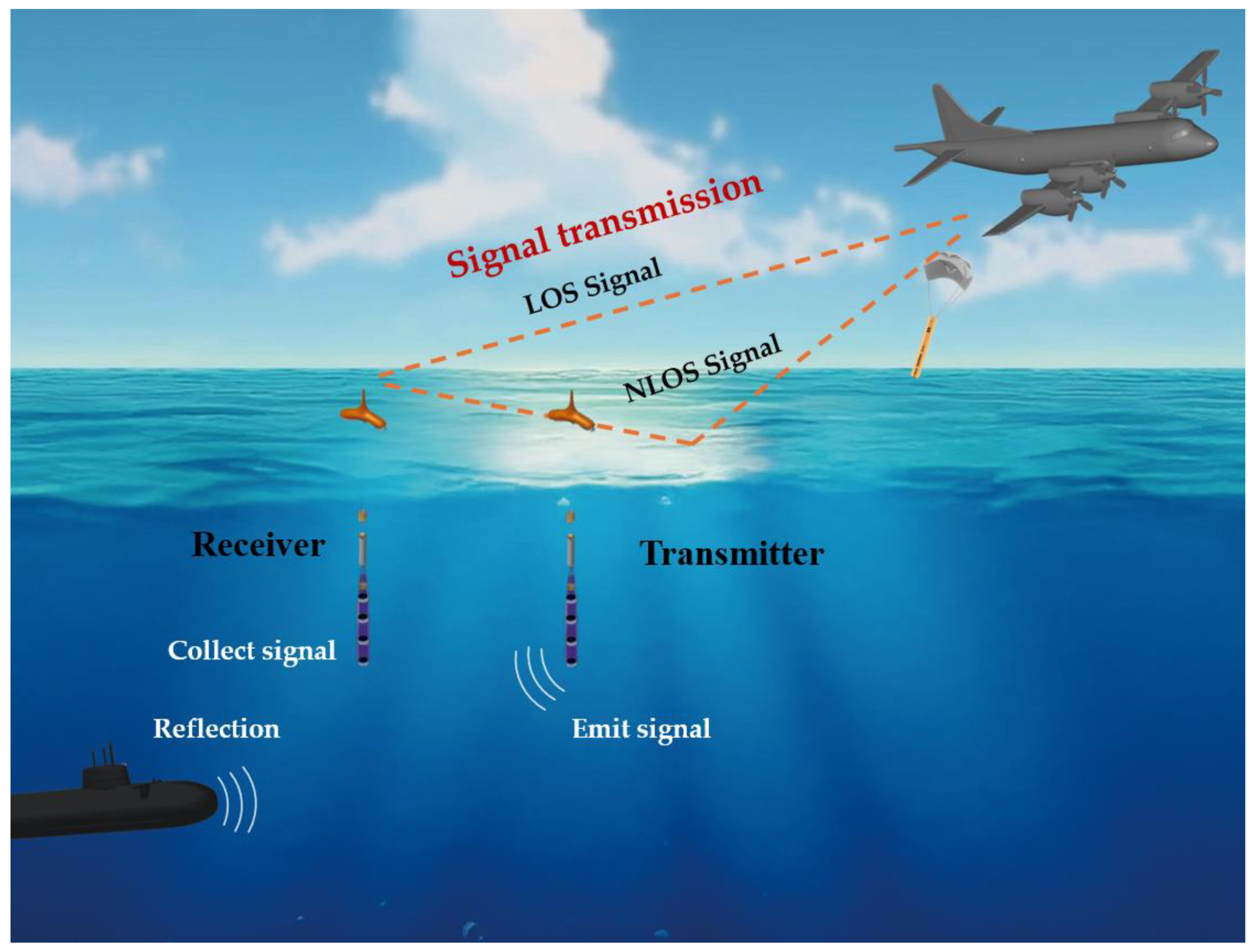
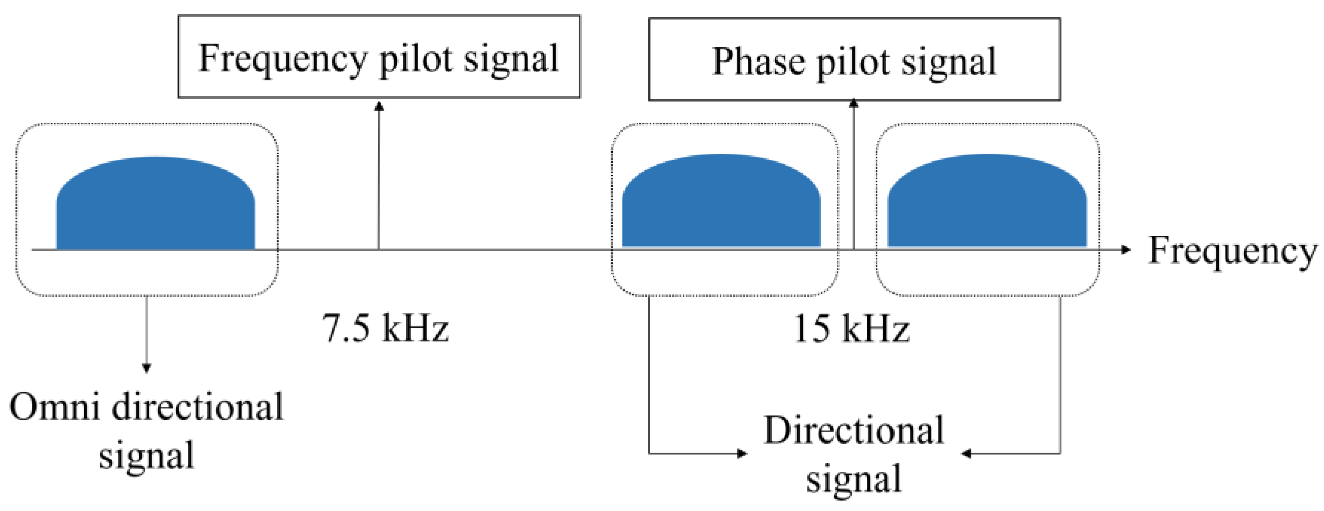
2.1. Traditional DIFAR Sonobuoy Transmission and Reception Technique Based on FDM

DIFAR sonobuoys employ FDM to convert various signals into a single composite signal for transmission. As illustrated in Figure 2, DIFAR sonobuoys collect both omnidirectional acoustic signals and two-channel directional signals. The collected omnidirectional signals are modulated to occupy the low-frequency band, whereas the directional signals are modulated to reside in the vicinity of the 15 kHz band. However, the single channel resulting from FDM requires a relatively large data amount of data transmission, and the transmitted signals are distinguishable within the predetermined frequency band, thereby exhibiting low security [6].

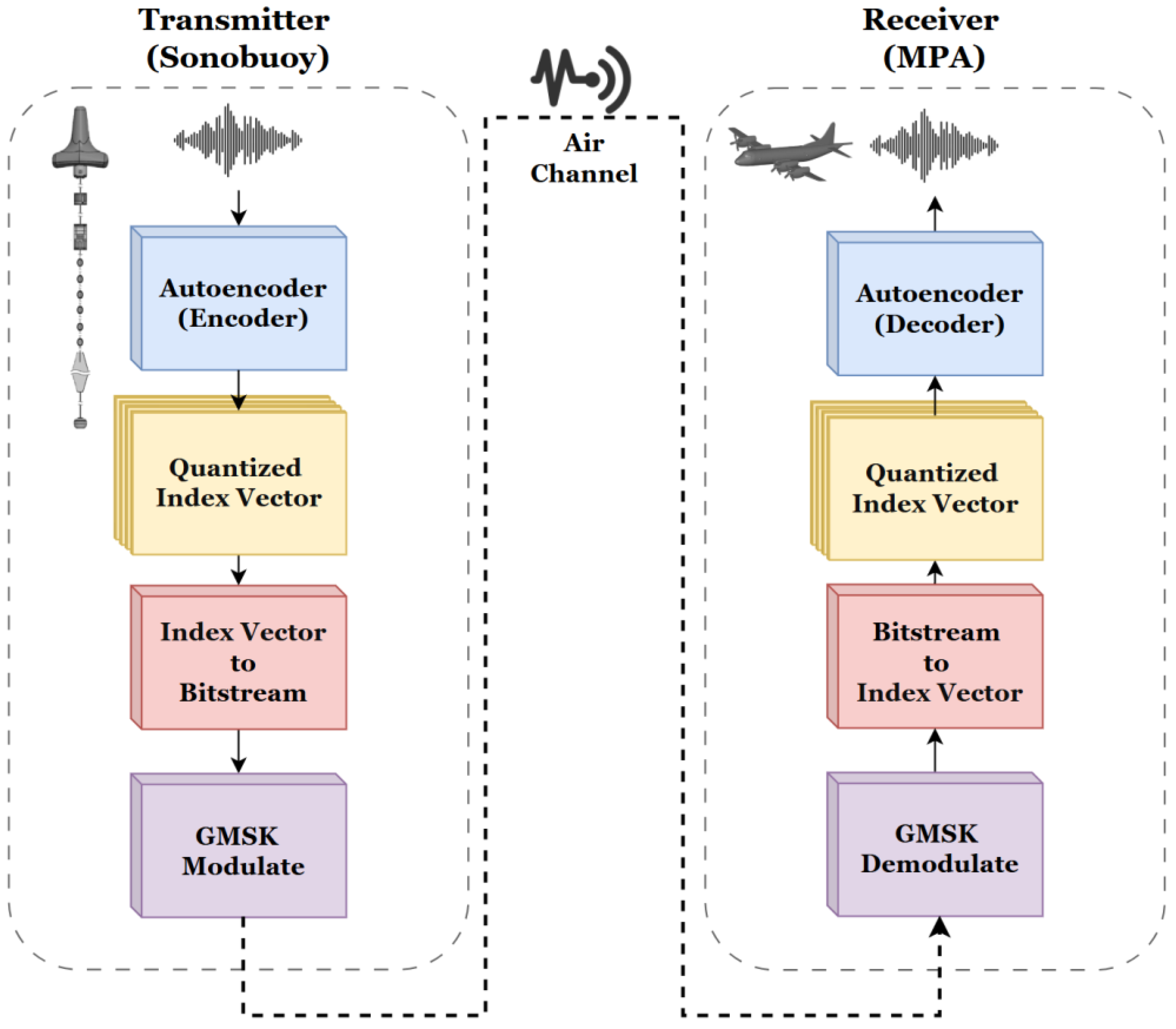
2.2. DIFAR Sonobuoy Transmission and Reception System Based on Autoencoder

An autoencoder is a representative neural network architecture in unsupervised learning, primarily utilized for data compression and reconstruction. Fundamentally, an autoencoder processes input data through two stages: an encoder and a decoder. The encoder compresses the input data into a latent vector, and the decoder reconstructs an output that is similar to the original data based on this latent vector. Additionally, because reconstructing the signal from the latent vector requires knowledge of the decoder structure used during training, even if a third party acquires the transmitted latent vector, they cannot decode the original signal. The structure of the DIFAR sonobuoy transmission and reception system utilizing the advantages of the autoencoder can be described as follows:

• Encoder (Sonobuoy): Maps the collected acoustic signal to a low-dimensional latent space, extracting essential features of the data. The encoder compresses the data, transforming the input into a latent vector that is trained to encapsulate the critical information of the data.
• Latent Vector (Wireless Communication): The latent vector generated by the encoder is a compressed representation of the original data’s key information. This compressed latent vector, requiring minimal data for transmission, is sent wirelessly from the sonobuoy to the MPA, enabling secure and effective data transfer for further analysis and reconstruction.
• Decoder (MAP): The decoder reconstructs an acoustic signal similar to the original from the latent vector. By performing the inverse process of the encoder, it reconstructs the structure of the input data and restores the original signal based on the received latent vector.

By integrating autoencoder techniques, previous studies [6] demonstrated that the amount of data transmitted could be reduced by approximately 130-fold compared to conventional 8-bit quantization methods while maintaining comparable signal reconstruction performance. Furthermore, this approach enhances data security since reconstructing the original signal requires access to the decoder structure used during training. The model structure of the existing autoencoder-based method for enhancing the DIFAR sonobuoy transmission and reception system is presented in

Table 1. Model structure of the conventional DIFAR sonobuoy autoencoder [6].

Encoder (Dim)	Decoder (Dim)
Noisy input (3125)	Latent vector (10)
Linear (3125–1000)	Linear (10–100)
ReLU	ReLU
Linear (1000–500)	Linear (100–500)
ReLU	ReLU
Linear (500–100)	Linear (500–1000)
ReLU	ReLU
Linear (100–10)	Linear (1000–3125)
ReLU	Tanh
Latent vector (10)	Output (3125)

.

2.3. Residual Vector Quantization (RVQ)

RVQ is a technique proposed to efficiently compress high-dimensional data. The core idea of RVQ initially involves quantizing the data vector in the first stage, calculating the resulting residual, and then using this residual as the input for the subsequent quantization stage. In subsequent stages, the residuals are continuously quantized in the same manner, with the magnitude of the residuals progressively decreasing at each stage. This iterative process ultimately achieves quantization performance that closely approximates the original data vector. When applied to neural network-based audio codecs, RVQ is effectively utilized for high-quality audio reconstruction. The quantization process of RVQ is outlined in Algorithm 1 [9,10,12].

Algorithm 1: Residual vector quantization (RVQ)

1: RVQ(y, $Q_1$, $Q_2$, …, $Q_{N_q}$) 2: Input: $y=enc\left(x\right)$, where $y$ is the encoder output vector 3: Input: $Q_i$ for $i=1, \dots , N_q$ (vector quantizers or codebooks) 4: Output: Quantized Vector $\widehat{y}$ 5: Initialize: $\widehat{y}\leftarrow 0.0$, $residual\leftarrow y$ 6: for $i$ = 1 to $N_q$ do 7:       $\widehat{y}+=Q_i\left(residual\right)$ 8:        $residual-=Q_i\left(residual\right)$ 9: return $\widehat{y}$

2.4. Quantization Compensation Module

Recent studies have focused on developing compensation modules to predict and correct errors that occur during the quantization process. These compensation modules are trained in conjunction with the encoder and decoder, with an emphasis on minimizing errors arising from quantization. Specifically, quantization inevitably results in the loss of detailed signal information, leading to discrepancies between the original and reconstructed signals. Consequently, a method capable of compensating for these losses is essential.

The quantization–compensation module proposed in LightCodec [14] employs a shallow convolutional neural network to predict and reduce errors that occur during the quantization process. This module is positioned immediately after the quantization layer to correct errors arising from the quantized latent vectors. Specifically, the quantization–compensation module consists of two shallow convolutional layers and takes the reconstructed latent vector as input to calculate the expected quantization error. The predicted error is then added to the reconstructed latent vector before being transmitted to the decoder. Through this process, the decoder can minimize the losses caused by quantization, thereby restoring signals that are closer to the original. Furthermore, to enable the LightCodec compensation module to accurately predict and correct quantization errors, a loss function is defined. In general, MSE loss is utilized to train the system in a way that minimizes the difference between the encoder’s output and the quantization results processed by the compensation module. This MSE loss allows the quantization–compensation module to more precisely predict and correct quantization errors, ultimately contributing to enhanced reconstruction quality for the decoder.

2.5. Pruning to Lighten Neural Network Models

Artificial neural network models are typically over-parameterized, resulting in inefficient use of memory and computational resources. To address this inefficiency, various research efforts have been proposed. In this study, we reference the model pruning technique developed by Han et al. [19]. This method significantly reduces memory usage and computational load by eliminating non-essential connections through pruning techniques after network training, achieving a ninefold reduction in the number of parameters for AlexNet [20] and a thirteenfold reduction for VGG-16 [21], all while maintaining the accuracy of the original models. The core of this approach consists of three main stages: network training, removal of non-essential connections, and retraining of the pruned network. Through pruning and retraining, the final network adopts a sparse structure, thereby substantially enhancing the network’s efficiency.

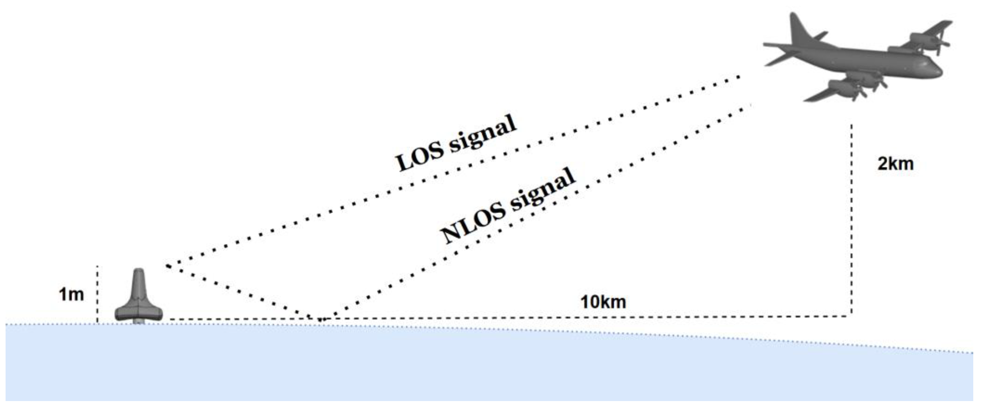
2.6. Airchannel Modelling for Realistic Communication Experiments

To accurately imitate realistic communication environments within the communication system between sonobuoys and MPA, air channel modeling that reflects actual environmental conditions is essential. Extensive research has been conducted on air channel modeling [22,23,24], with the free-space path loss and two-ray models being prominent examples. These models offer the advantage of incorporating signal reflections from the ground surface, thereby capturing the effects of signal propagation more effectively.

Recent studies have extended the traditional two-ray model to develop the Curved-Earth Two-Ray Model [23,24], which accounts for the curvature of the earth and facilitates precise channel modeling in both terrestrial and aerial communication environments. The Curved-Earth Two-Ray Model was primarily developed to analyze air–ground communications in unmanned aerial systems (UAS). This model assesses the attenuation characteristics of the communication channel by including both the direct path and the ground-reflected path, effectively reflecting path differences due to the curvature of the earth and the conditions of ground reflections. Research in [23,24] has demonstrated that this model effectively simulates complex phenomena, such as reflection effects caused by path differences over land and water surfaces, thereby providing a more accurate representation of signal behavior in real-world scenarios.

3. Proposed Method for Autoencoder-Based DIFAR Sonobuoy Signal Transmission and Reception Systems Considering Air Channel Modeling

In this paper, we propose a signal compression autoencoder tailored for the transmission and reception environment of DIFAR sonobuoys, along with an air channel model communication system to validate its effectiveness. The overall system flow is as follows. As illustrated in Figure 3, the sonobuoy collects underwater acoustic signals, which are then converted into QIV (Quantized Index Vectors) through an encoder mounted on the sonobuoy. These vectors are subsequently transformed into bit-streams and modulated into signals suitable for wireless communication using GMSK (Gaussian low-pass-filtered Minimum Shift Keying) digital modulation. The modulated signals are transmitted to an MPA, where the received GMSK signals are demodulated to restore the bitstreams back into QIV. Then QIV are processed by a decoder to reconstruct the original acoustic signals.

Performance improvement of the proposed system is influenced by the improved design of the deep learning model, which will be discussed in detail in Section 3.1. Additionally, since sonobuoys are battery-operated devices, minimizing computational load and reducing the number of parameters is essential to overcome operational time constraints. Consequently, the encoder of the proposed system has been optimized using pruning techniques, and the optimization algorithms and specific methodologies employed are elaborated in Section 3.2. Furthermore, considering the communication environment between sonobuoys and MPA, we have designed an air channel model that accurately reflects the signal characteristics during actual wireless transmission. Detailed aspects of the air channel model design are addressed in Section 3.3.

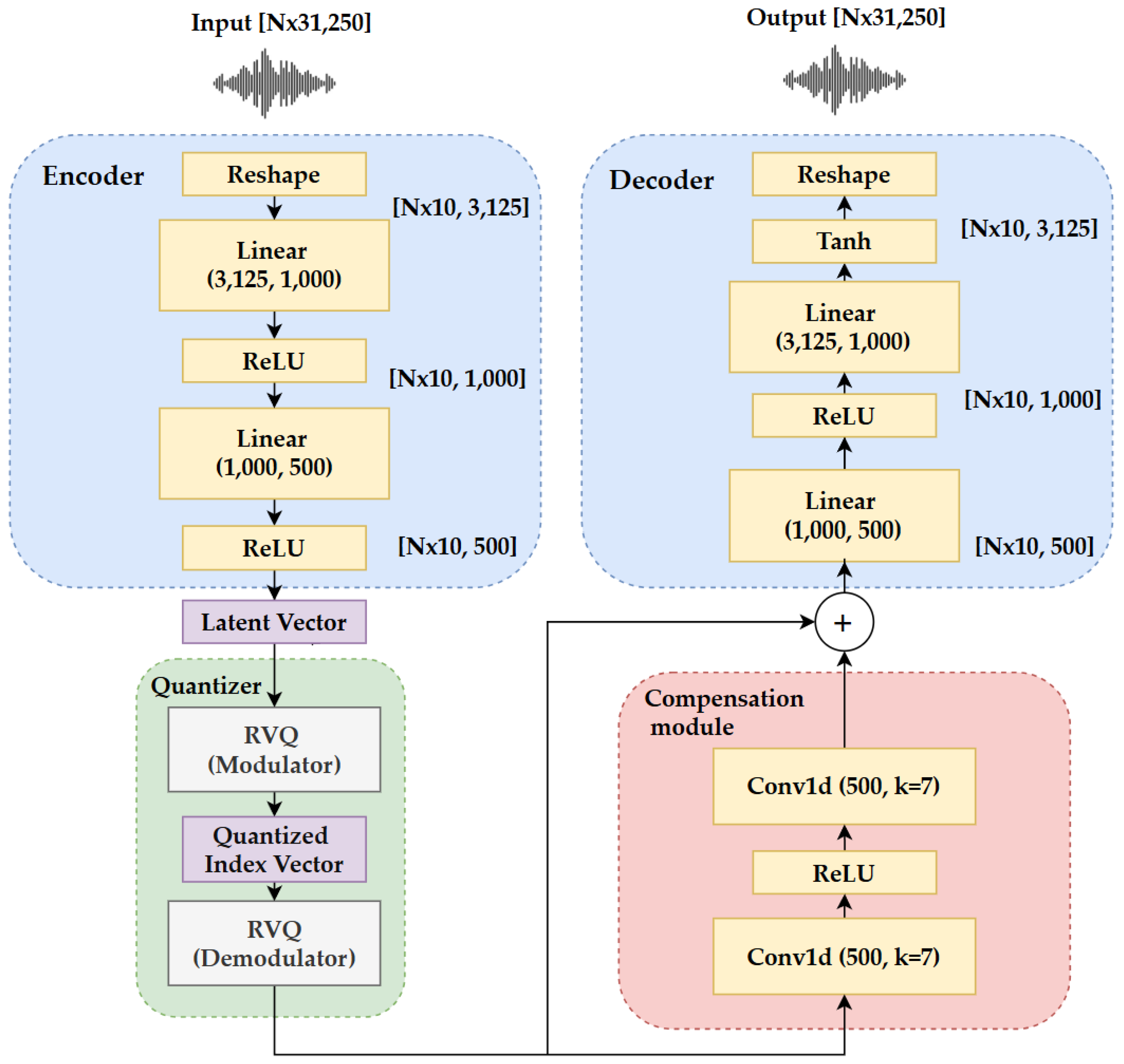
3.1. Enhanced Autoencoder-Based Neural Network Architecture Combining RVQ and CM

In this study, to efficiently compress and transmit underwater acoustic signals collected by DIFAR sonobuoys, we propose a novel autoencoder-based neural network that integrates RVQ and a CM with the autoencoder architecture in [6]. Figure 4 illustrates the structure of the proposed autoencoder-based system.

The proposed model is tailored for the characteristics of sonobuoy signals, which differ significantly from general acoustic signals, such as music or speech. General acoustic signals exhibit complex and dense time-frequency patterns, requiring neural codecs [9,10,11,13,14] with convolutional neural network (CNN)-based architectures to capture intricate features across the entire signal. Accordingly, general acoustic signal compression and reconstruction models often utilize multi-layer CNNs with strided convolutions to progressively reduce the temporal resolution while extracting features across multiple channels. Although effective for general audio signals, these architectures demand high computational resources and power, making them unsuitable for environments with limited power availability, such as sonobuoy systems.

In contrast, the signals used by sonobuoys, such as Continuous Wave (CW) and Linear Frequency Modulation (LFM), have simple and sparse time-frequency characteristics. CW signals concentrate energy at specific frequencies, while LFM signals exhibit linear frequency changes over time. Leveraging these properties, the proposed model avoids complex CNN layers and instead uses linear layers to process the signals. The input is divided into 0.1-second segments (3125 samples at a sampling frequency of 31,250 Hz), resulting in low-dimensional input due to the short signal length. This enables efficient compression and feature extraction by processing the data in parallel through linear layers.

Furthermore, the proposed model integrates RVQ and a CM to enhance compression and reconstruction performance. Unlike general audio codecs that rely on deep and complex architectures, the proposed model is lightweight and tailored to address the power and computational constraints of battery-operated sonobuoy systems. By focusing on the simplicity and sparsity of sonobuoy signals, the proposed model achieves efficient signal processing with a much lower computational load than conventional CNN-based codecs.

The proposed model consists of an encoder, quantizer, compensation module, and decoder. First, the encoder compresses the collected acoustic signal into a low-dimensional feature vector. The encoder architecture utilizes multiple linear layers and the ReLU activation function to transform the input signal into a latent vector. While the process is similar to previous approaches, the proposed model differs in that it does not directly reduce the latent space to 10 dimensions. Instead, it first compresses the input to 500 dimensions and then converts it into a 10-dimensional QIV through RVQ. This intermediate step of reducing to 500 dimensions offers an advantage over the conventional method [6], which compresses the input directly to 10 dimensions using stacked linear layers. By maintaining a 500-dimensional latent space, the model can preserve critical information in the signal more effectively.

RVQ is a multi-stage quantization technique that iteratively reduces residual errors to improve quantization accuracy. Through this process, the 500-dimensional latent vector generated by the encoder is represented as a compressed 10-dimensional QIV. This approach prevents the loss of critical information that may occur in conventional methods [6], where the input signal is directly reduced to 10 dimensions using stacked linear layers, and ensures more stable compression. Subsequently, the QIV is reconstructed into a latent vector through the RVQ demodulator and then passed to the decoder for further processing.

The reconstructed latent vector is fed into the decoder, with an additional CM employed to correct errors introduced during the quantization process. The CM consists of shallow 1D convolution layers, designed to compensate for errors arising during the quantization and reconstruction stages, thereby improving the quality of the final reconstructed signal. The correction signal generated by the CM is integrated with the input to the decoder, allowing the decoder to ultimately reconstruct the signal in a form closely resembling the original acoustic signal.

Moreover, the proposed method achieves a higher compression ratio compared to the conventional approach [6]. In the conventional method, the latent vector in the latent space is represented using 16 bits, whereas the proposed RVQ method improves the compression ratio by representing the signal as a 10-bit QIV. RVQ sets the size of the index vector to 1024 (10 bits) at each stage and progressively reduces the residuals over a total of 10 stages. This facilitates more efficient acoustic signal transmission between DIFAR sonobuoys and MPAs.

3.2. Description of the Pruning Algorithm

Sonobuoys are battery-powered devices, making energy efficiency a critical factor directly linked to operational duration. To operate effectively within a limited power environment, this study aims to minimize the computational load and the number of parameters of the encoder mounted on the sonobuoy by applying an unstructured pruning technique that removes unnecessary weights. The proposed pruning technique consists of initial training stages, pruning and retraining stages, and iterative pruning with performance evaluation. It is designed to maximize efficiency while minimizing performance degradation through iterative pruning.

Furthermore, the acoustic signals collected by the sonobuoy are transmitted to an MPA for underwater target detection and analysis. Since the decoder is mounted on the MPA, which receives a continuous power supply, it is not constrained by energy consumption. Therefore, this study focuses on applying pruning techniques exclusively to the encoder, which is mounted on the battery-powered sonobuoy, to maximize energy efficiency and achieve high performance.

3.2.1. Early Learning Phase

In the initial training phase, the model is thoroughly trained without pruning to ensure stable learning of the data characteristics. During this process, the best evaluation loss is recorded and used as a benchmark for maintaining performance during the pruning process. Upon completion of this stage, the model becomes ready for the application of pruning.

3.2.2. Pruning and Retraining Steps

Upon completion of the initial training, the pruning phase commences in earnest. Pruning is carried out by unstructured removal of 10% of the model’s weights at each epoch. Following pruning, retraining is conducted to compensate for any performance degradation resulting from the pruning process. During the retraining phase, the evaluation loss after pruning is compared to the best evaluation loss recorded during the initial training, with the goal of restoring performance to a level comparable to that before pruning. If the evaluation loss remains within a certain permissible range (approximately 0.5%), the next pruning iteration may proceed. However, if the performance degradation caused by pruning exceeds the allowable range, pruning is temporarily halted, and additional retraining is performed to recover performance. Furthermore, if the evaluation loss measured during retraining is lower than the previously recorded best evaluation loss, the best evaluation loss is updated accordingly.

3.2.3. Pruning Iterations and Performance Evaluation

If the evaluation loss consistently remains within the permissible range during the pruning and performance recovery processes, pruning is performed iteratively. Following each pruning iteration and the subsequent performance recovery phase, if the performance no longer improves due to pruning or if stable performance cannot be maintained, the pruning process is halted, and the model from the preceding pruning stage is determined as the final model.

3.3. Air Channel Model Simulating a Maritime Communications Environment

To accurately replicate the realistic communication environment between sonobuoys and MPA, we employed an air channel model that combines free-space path loss and the Curved-Earth Two-Ray Model [23]. This model simulates multipath effects and signal attenuation by considering the curvature of the earth and ground surface reflections. Moreover, the model is advantageous for replicating the signal path characteristics that occur in maritime communication environments by incorporating various paths and surface reflection effects.

The free-space path loss model predicts signal attenuation in an ideal linear path between the transmitter and receiver, inversely proportional to the square of the distance, thereby estimating signal loss. However, this model does not sufficiently account for practical complexities, such as ground surface reflections, which occur in marine environments. To address these limitations, we incorporated the Curved-Earth Two-Ray Model.

The Curved-Earth Two-Ray Model divides the signal paths into two routes that account for the curvature of the earth: the LOS path and the NLOS ground reflection path. By considering the path differences caused by reflections, the model simulates multipath interference and signal attenuation. It calculates the characteristics of the signal path, including the time delays and phase differences of the two paths. The primary equations of the model are as follows:

$$h_{2Ray}\left(t,\tau \right)={\alpha }_0\left(t\right)\exp \left(j{\phi }_0\left(t\right)\right)\delta \left(\tau -{\tau }_0\left(t\right)\right)+{\alpha }_1\left(t\right)\exp \left(j{\phi }_1\left(t\right)\right)\delta \left(\tau -{\tau }_1\left(t\right)\right) ,$$

(1)

where $t$ represents the continuous time variable, describing the dynamic behavior of the signal over time, while $\tau$ refers to the delay time, which indicates the time it takes for the signal to travel along a specific path. Specifically, the delay times of the LOS path, ${\tau }_0\left(t\right)$ and the NLOS reflection path ${\tau }_1\left(t\right)$ are expressed as follows:

$${\tau }_0\left(t\right)={\displaystyle \frac{R_1}{c}} , {\tau }_1\left(t\right)={\displaystyle \frac{R_2}{c}},$$

(2)

where $R_1$ and $R_2$ represent the LOS and NLOS path distances and $c$ is the speed of light.

The amplitude of the LOS signal, ${\alpha }_0\left(t\right)$ is influenced by free-space path loss and is expressed as:

$${\alpha }_0\left(t\right)={\displaystyle \frac{c}{4\pi f_c{R}_1}},$$

(3)

where $f_c$ is the carrier frequency. In contrast, the amplitude of the reflected signal ${\alpha }_1\left(t\right)$ is influenced by a combination of the reflection coefficient $\mathsf{\Gamma }$, the surface roughness attenuation factor $r_F,$ and the divergence factor $D_k$, and is expressed as:

$${\alpha }_1\left(t\right)={\displaystyle \frac{c}{4\pi f_c{R}_2}} ·\mathsf{\Gamma }·r_F·D_k ,$$

(4)

where the reflection coefficient $\mathsf{\Gamma }$ accounts for the sea surface properties, specifically the relative permittivity of seawater $({ϵ}_r=81)$, the conductivity $(\sigma =5 \mathrm{S}/\mathrm{m}$, Siemens per meter) [25], and the incidence angle. Meanwhile, the surface roughness attenuation factor $r_F$ quantifies the signal loss caused by the roughness of the sea surface, while the divergence factor $D_k$ incorporates the geometric spreading effect of the curved reflection path [23,26]. The phase variations of the LOS and NLOS paths are represented as ${\phi }_0\left(t\right)$ and ${\phi }_1\left(t\right)$, respectively, and are calculated based on the path lengths $R_1$ and $R_2$. These phase shifts are expressed as follows:

$${\phi }_0\left(t\right)=-{\displaystyle \frac{2\pi f_c{R}_1}{c}}, {\phi }_1\left(t\right)=-{\displaystyle \frac{2\pi f_c{R}_2}{c}},$$

(5)

Together, these parameters delay times, amplitudes, and phase variations, enabling a more realistic representation of signal attenuation and multipath interference in maritime communication environments.

4. Experimental Results

4.1. Training Results of the Proposed Models With or Without Pruning (Techinique)

4.1.1. Experimental Setup for Deep Neural Network Model

In this study, training was conducted using acoustic signals from a bistatic sonobuoy environment employed in the previous DIFAR sonobuoy signal transmission and reception autoencoder model [6]. The experimental data were generated through bistatic simulations in an underwater environment, and the transmitted signals comprised two types: CW and LFM. The positions of the transmitter and receiver were fixed, and the maximum distance between the target and the sonobuoys was limited to 9 km. The maneuvering range of the target was set between 50 m and 150 m to model the characteristics of reflected signals occurring at various distances.

The additional conditions for generating simulation data are summarized in

Table 2. Parameters for the bistatic sonobuoy signal collection simulation.

	CW	LFM
Center frequency (Hz)	3500, 3600, 3700, 3800
Bandwidth (Hz)	-	400
Pulse duration (s)	0.1, 0.5, 1
Sampling frequency (Hz)	31,250
Total Time (h)	43	43

. Signal collection was organized into various scenarios, with each scenario featuring randomly set target positions. The collected data were stored as approximately 13s WAV files. The entire training dataset comprised approximately 86 h of data, and an additional evaluation set of approximately 14 h was used to assess the convergence of model training. The proposed autoencoder model was developed and trained using PyTorch 1.10.1 on an NVIDIA RTX A6000 GPU to handle the extensive dataset efficiently. A ray tracing technique was applied in data generation to reflect underwater acoustic propagation paths, adhering to the same conditions in [6].

The input signals used for training were normalized to a range of −1 to 1 for each file and then segmented into units of 3125 samples, corresponding to 0.1 s. These segmented input data were stacked to facilitate the effective learning of the model for the temporal patterns inherent in underwater acoustic signals during training. The optimizer employed in training was the Adam [27] optimization algorithm, configured to simultaneously update the parameters of the encoder, decoder, and quantizer. The Adam optimizer was initialized with a learning rate of 0.0003 and momentum coefficients $\left({\beta }_1.{\beta }_2\right)=(0.5, 0.9)$ to enhance training stability and promote rapid convergence, referencing the optimizer parameters from Encodec [10]. Furthermore, when the evaluation loss did not improve during the training process, the learning rate was adjusted to finely optimize the performance of the model. To achieve this, a learning rate decay factor of 0.9 was applied, reducing the learning rate by 10% each time the evaluation loss did not decrease. This learning rate adjustment strategy contributed to the stable convergence of the model and the attainment of improved performance. Subsequently, the loss function used for training was structured to enable the model to effectively learn signal reconstruction. The loss function comprised a total of three loss components, which are as follows:

• Reconstruction Loss: For signal reconstruction loss, the MSE loss function was utilized. This function is employed to minimize the discrepancy between the final output of the model and the input data. MSE is calculated by averaging the squared differences between the input signal and the reconstructed signal.
• Quantization Penalty: This component aims to minimize the error between the quantized vectors generated by RVQ and the original latent vectors. It is defined as the average of the cumulative errors across each quantization layer.
• CM Loss: To minimize errors arising during the quantization process, the loss is defined by comparing the original latent vectors with the output of the CM using MSE. A specific weight ($\alpha$ = 0.01) is multiplied with the compensation loss and added to the overall loss. This weight was set empirically.

The final loss function is defined as follows:

$$Total Loss=Reconstruction Loss+Quantization Penalty+\alpha CM Loss.$$

(6)

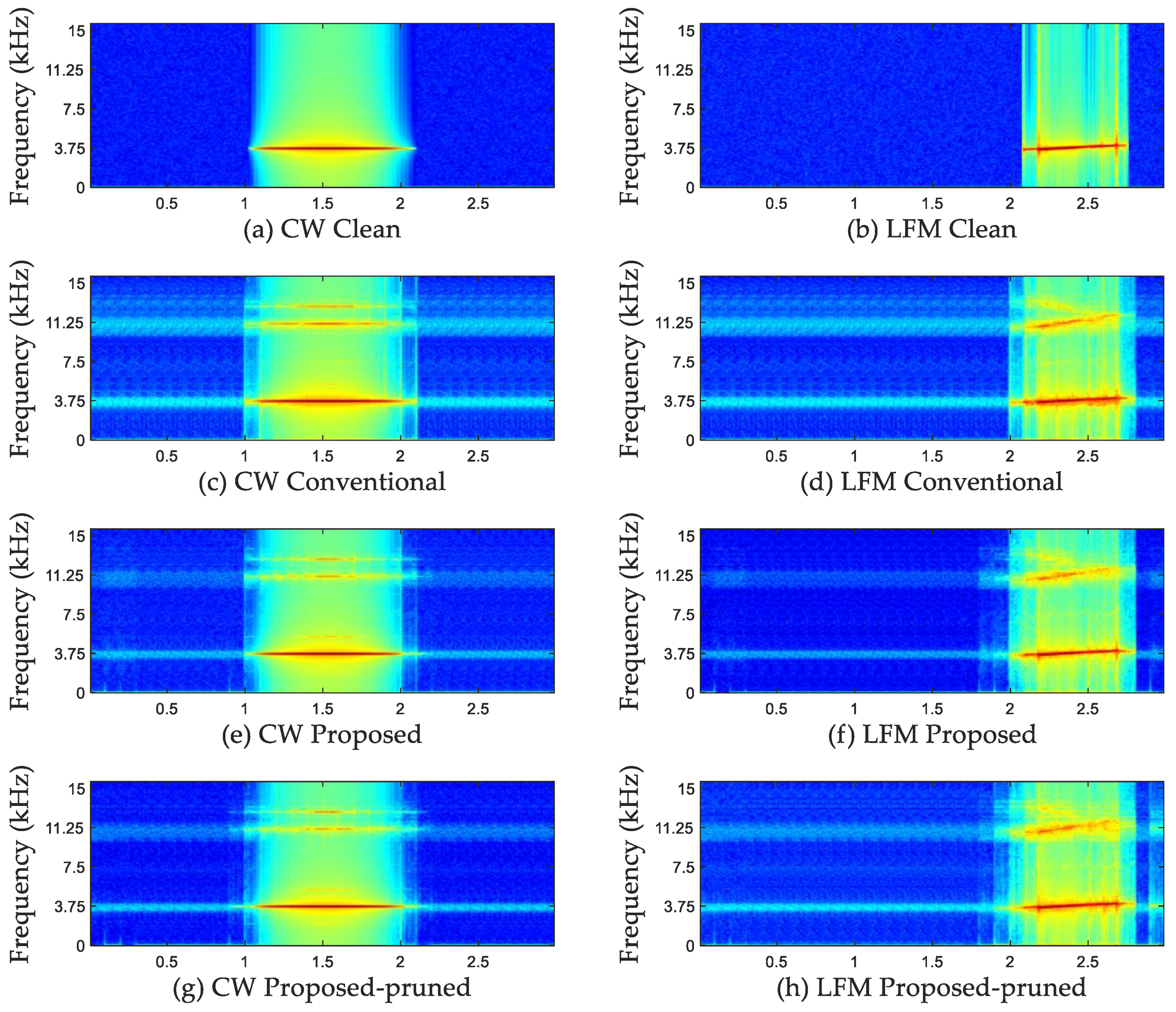
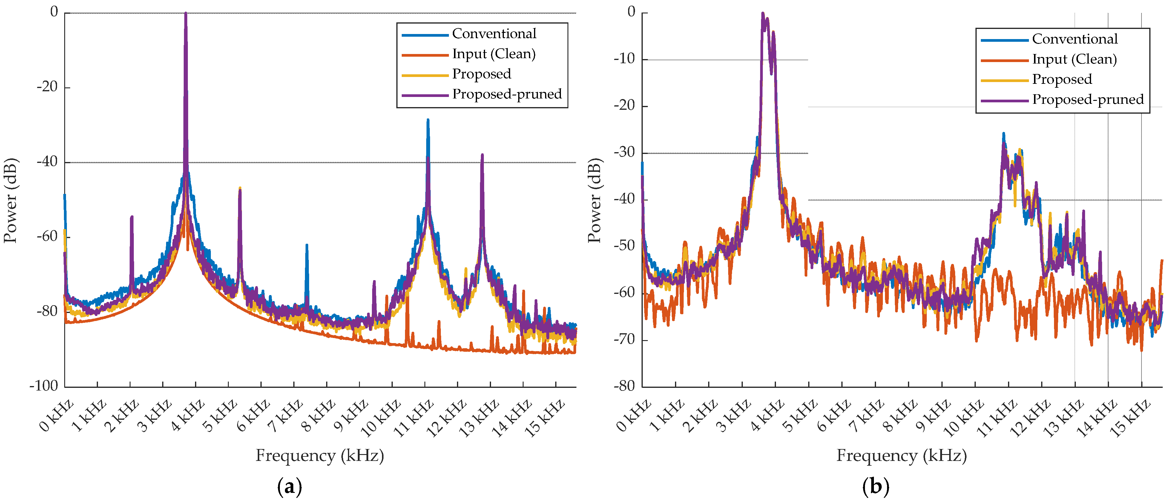
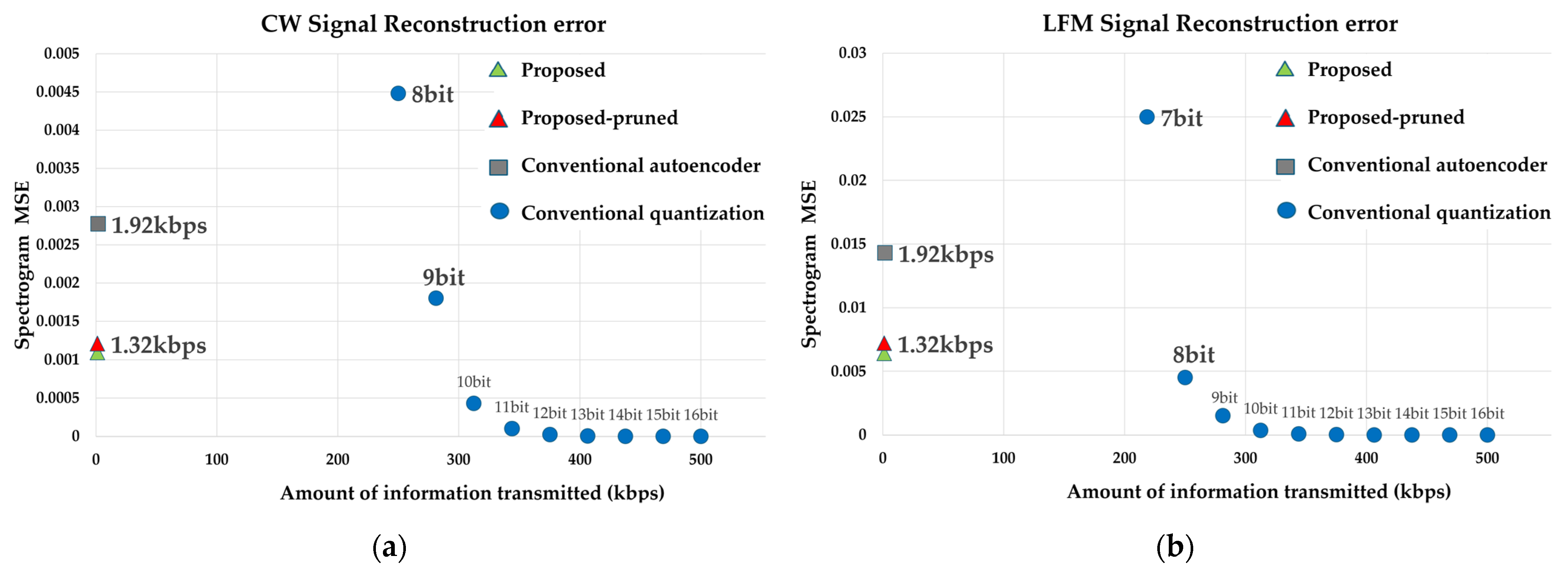
4.1.2. Experimental Results of Deep Neural Network Model

To design a system suitable for the power-constrained environment of sonobuoys, pruning was applied only to the encoder among the encoder and RVQ. This is because pruning is challenging for RVQ due to its structural characteristics. RVQ operates based on a fixed codebook at each stage, and this codebook consists of static data that is not updated, like trainable weights, during the learning process. In contrast, the encoder is composed of a deep learning network, allowing pruning techniques to effectively reduce trainable weights and computational requirements. Therefore, pruning was applied to the encoder to design a lightweight model suitable for the constrained environment of sonobuoys.

The pruning results are summarized in

Table 3. Computational and parameter requirements for the model in sonobuoy systems.

Model Encoder	Parameter (Encoder)	Parameter (RVQ)	MMACs (Encoder)	MMACs (RVQ)
Conventional [6]	3.68 M	-	36.82	-
Proposed	3.63 M	5.12 M	36.30	51.2
Proposed–Pruned	1.03 M	5.12 M	10.30	51.2

, where the computational requirements are measured in Mega Multiply-Add Operations per Second (MMACs) for processing 1-second audio signals. The computational measurements for the encoder and RVQ in the proposed system show that additional RVQ parameters of 5.12 million and a computational requirement of 51.2 MMACs were introduced compared to the conventional method [6]. However, these values remain significantly lower than those of LightCodec [14], a state-of-the-art lightweight neural codec for audio signals, which requires 820 MMACs. These results demonstrate that the proposed system is efficient and well-suited for environments with limited power and computational resources, such as sonobuoy operations.

To evaluate the performance of the proposed neural codec system, we quantitatively measured the Spectrogram MSE (MSE), Log Spectral Distance (LSD), and Signal-to-Noise Ratio (SNR) between the reconstructed signals and the original input signals. Additionally, a subjective comparison was conducted through visual analysis of the spectrograms. Performance evaluation was carried out using approximately 0.5 h of CW and LFM signals, which were not included in the training set, totaling 1 h of evaluation data.

Additionally, the spectrogram MSE is calculated as the mean squared error between the amplitude spectra of the original and reconstructed signals. It is defined by the equation:

$$MS{E}_{spectrogram}={\displaystyle \frac{1}{N_{frame}}} \sum _{j=1}^{N_{frame}}({\displaystyle \frac{1}{N-1 }} \sum _{k=2}^N{\left(\left|X_k^j\right|-\left|Y_k^j\right|\right)}^2 ) ,$$

(7)

where $N_{frame}$ represents the total number of frames, and $N$ is the number of samples per frame (corresponding to the FFT size). The term $\left|X_k^j\right|$ refers to the amplitude spectrum of the original signal at frequency index $k$ for frame $j$, while $\left|Y_k^j\right|$ denotes the amplitude spectrum of the reconstructed signal at the same frequency and frame. The summation starts from $k=2$ to exclude the DC component, focusing only on the non-DC frequency components.

Table 4. Overall signal performance comparison of proposed autoencoder models with conventional methods.

Method	Signal Type	Spectrogram MSE	LSD (dB)	SNR (dB)
Conventional [6]	CW	0.00277	1.19	25.93
	LFM	0.01428	1.19	17.66
Proposed	CW	0.00109	1.13	29.19
	LFM	0.00639	1.10	21.56
Proposed–Pruned	CW	0.00128	1.15	28.59
	LFM	0.00719	1.12	21.08

presents the results of this quantitative evaluation, including a comparison with the existing DIFAR sonobuoy-based neural codec [6]. Furthermore, the proposed method incorporates the results of encoder optimization achieved through parameter pruning, which is known as Proposed–Pruned.

The proposed method demonstrated a 60.58% reduction in Spectrogram MSE for CW signals and a 55.22% reduction in Spectrogram MSE for LFM signals compared to the existing method. Simultaneously, improvements in LSD and SNR metrics were observed. The Proposed–Pruned model maintained a comparable level of quality to the proposed method without significant performance degradation, further proving its efficiency. Furthermore, the quantitative metrics for target signals, which are measured only in the target interval, are presented in

Table 5. Performance comparison of proposed autoencoder models measured only in target interval with conventional methods.

Method	Signal Type	Spectrogram MSE	LSD (dB)	SNR (dB)
Conventional [6]	CW	0.00418	1.26	25.94
	LFM	0.02153	1.24	17.74
Proposed	CW	0.00204	1.21	29.22
	LFM	0.00812	1.18	21.62
Proposed–Pruned	CW	0.00254	1.23	28.62
	LFM	0.00918	1.20	21.14

, which supports the improvement tendency in Table 4.

The spectrogram analysis in Figure 5. reveals no significant visual differences between the proposed method and its lightened version. However, when comparing the proposed method with the existing method [6], a substantial reduction in reconstruction errors in non-signal (or background noise only) regions was observed for both CW and LFM signals using the proposed method. Additionally, in the existing method (c), frequency spectrum distortions were evident near the target frequency band at 3.75 kHz, resulting from incomplete signal reconstruction. These distortions introduced unwanted frequency components, degrading the quality of the reconstructed signal. In contrast, the proposed method effectively suppressed such distortions, maintaining a signal shape similar to the input signal even in regions with target signals. Consequently, the proposed method provided high-quality reconstructions closer to the original signal.

This superiority is further demonstrated in the frequency analysis results presented in Figure 6. For CW signals, the proposed methods showed frequency characteristics near the target band of 3.75 kHz that were more similar to the input signal than the existing method. For LFM signals, while the existing method exhibited better resemblance to the original signal in the 10–11 kHz frequency range, the proposed methods showed higher similarity across all other frequency bands. This indicates that the proposed methods effectively maintain signal accuracy over a broader frequency range.

In addition, the results in Figure 7 show that the proposed and Proposed–Pruned methods significantly reduced reconstruction errors (Spectrogram MSE) compared to the existing method while demonstrating high transmission efficiency. Specifically, for CW signals, the proposed method reduced reconstruction errors by approximately 60.65% compared to the existing method, and the Proposed–Pruned method achieved a reduction of about 53.79%. For LFM signals, the proposed method recorded a reduction of approximately 55.25%, while the Proposed–Pruned method achieved a 49.65% reduction. These results clearly confirm that the proposed methods improved both reconstruction accuracy and transmission efficiency compared to the existing method.

4.2. Assessing the Corruption Impact of QIV in a Wireless Communication Environment

4.2.1. Experimental Setup for Air Channel Model

To evaluate the performance of the autoencoder-based neural codec system in the wireless communication environment between DIFAR sonobuoys and MPA, an air channel model simulating actual wireless communication conditions was developed. The purpose of this experiment was to analyze the impact of the Bit Error Rate (BER) of the Quantized Index Vector on the signal reconstruction performance of the neural codec. For this, the simulation was conducted in a simplified environment, with the air channel model configured based on the wireless communication parameters of the SSQ-573 DIFAR sonobuoy, as summarized in

Table 6. SSQ-573 DIFAR sonobuoy communication specifications.

Sonobuoy Characteristics
Telemetry (Digital Mode)	Coherent GMSK at 224 kbps
RF Channel	97 channels (136 MHz~173.5 MHz, 376 kHz spacing)
VHF Radiated Power	1 Watt nominal

[28].

As shown in Figure 8, the simulation was conducted in 2D space, and two experiments were carried out to validate the air channel model.

In the first experiment, the air channel model’s Pathloss was evaluated by configuring the positions of the sonobuoy and the MPA as follows. The sonobuoy’s X-axis position was fixed at 0 m, while its Y-axis position followed a Gaussian distribution within the range of 1 m to 0.5 m. The MPA’s X-axis position varied from 0 m to 10,000 m, while its Y-axis position followed a Gaussian distribution between 1950 m and 2050 m, introducing approximately 50 m of movement. Using these configurations, the Pathloss of the transmitted signal was measured, and a graph was generated with the X-axis representing the MPA’s X-axis position (distance) and the Y-axis representing the Pathloss values, validating the reliability of the air channel model.

In the second experiment, the system’s BER performance was evaluated under various SNR conditions. For this purpose, the sonobuoy’s X-axis and Y-axis positions were fixed at 0 m and 1 m, respectively, while the MPA’s X-axis and Y-axis positions were fixed at 10,000 m and 2000 m, respectively. In this fixed configuration, 150 different data samples were transmitted under varying SNR conditions, and the overall system performance was analyzed based on the resulting BER.

These two experiments were conducted to evaluate the reliability of the air channel model, which simulates a wireless communication environment, and to investigate the impact of BER degradation in wireless communication on the performance of autoencoder based acoustic signal compression and reconstruction model.

The wireless communication simulation process was as follows: the QIV was first converted into a 10-bit bitstream. The MATLAB Communications Toolbox was used to perform GMSK modulation and demodulation [29]. The GMSK modulation was configured with a bit rate of 224 kbps, a Bandwidth-Time Product of 0.5, and 16 samples per symbol to ensure signal integrity. At the receiver end, the GMSK demodulator was used with a Traceback Depth of 50 to accurately recover the signal.

The modulated signal was transmitted with a transmission power of 1 W. To simulate realistic wireless channel conditions, the signal was passed through an Additive White Gaussian Noise (AWGN) channel, introducing noise to the received signal. The demodulated bitstream was then compared with the original transmitted bitstream to evaluate the BER.

4.2.2. Experimental Results of Air Channel Model

The experimental setup modeled the channel characteristics by reflecting the dynamic positional changes of the sonobuoy and the aircraft. To validate this, the path loss of the air channel model was measured. The results of the path loss calculation are shown in Figure 9, illustrating the changes in path loss (dB) relative to the X-axis distance. The graph reflects dynamic variations caused by positional changes of the sonobuoy and the aircraft, showing minimal loss at closer distances and a gradual increase in loss as the distance grows. This validation confirmed the accuracy of the channel model and its suitability for BER measurements under realistic communication conditions.

To evaluate the degradation of the Quantized Index Vector under various conditions, this study measured the BER in an AWGN channel across different SNR conditions and analyzed its impact on the reconstruction performance of the neural codec. Quantitative evaluation metrics, including Spectrogram MSE, LSD, and SNR, were measured between the clean sonobuoy-collected signals and the reconstructed signals. The results are presented in

Table 7. Performance comparison of autoencoder models under AWGN channel with various SNR.

Method	Signal Type	AWGN SNR	BER (%)	Spectrogram MSE	LSD (dB)	SNR (dB)
Conventional	CW	0 dB	0.00006	0.00277	1.19	25.93
	LFM		0.00006	0.01428	1.19	17.66
Proposed	CW		0.00010	0.00113	1.12	29.19
	LFM		0.00010	0.00644	1.10	21.56
Proposed–Pruned	CW		0	0.00120	1.15	28.59
	LFM		0	0.00719	1.12	21.08
Conventional	CW	−1 dB	0.00019	0.00277	1.19	25.93
	LFM		0.00012	0.00142	1.19	17.66
Proposed	CW		0.00040	0.00129	1.13	29.03
	LFM		0.00040	0.00649	1.10	21.54
Proposed–Pruned	CW		0.00020	0.00123	1.15	28.54
	LFM		0.00040	0.00723	1.12	21.07
Conventional	CW	−2 dB	0.00192	0.00277	1.19	25.93
	LFM		0.00154	0.02075	1.19	21.22
Proposed	CW		0.00215	0.00209	1.13	29.14
	LFM		0.00225	0.00751	1.10	21.53
Proposed–Pruned	CW		0.00225	0.00304	1.15	28.55
	LFM		0.00266	0.00939	1.12	21.07
Conventional	CW	−3 dB	0.01126	0.04241	1.19	24.48
	LFM		0.01120	0.23350	1.19	16.67
Proposed	CW		0.01207	0.01681	1.14	25.28
	LFM		0.01125	0.01856	1.11	19.68
Proposed–Pruned	CW		0.01135	0.00765	1.16	27.83
	LFM		0.01156	0.01600	1.13	19.64
Conventional	CW	−4 dB	0.05318	0.20282	1.20	19.54
	LFM		0.05510	0.23350	1.24	12.70
Proposed	CW		0.05709	0.04873	1.17	20.36
	LFM		0.05831	0.05007	1.15	15.53
Proposed–Pruned	CW		0.05279	0.05013	1.18	19.82
	LFM		0.05862	0.06266	1.17	14.66
Conventional	CW	−5 dB	0.19361	0.81985	1.24	7.01
	LFM		0.19355	0.82393	1.24	3.76
Proposed	CW		0.19480	0.17122	1.26	11.75
	LFM		0.20289	0.17099	1.27	9.94
Proposed–Pruned	CW		0.19061	0.16431	1.26	11.39
	LFM		0.20401	0.16794	1.27	9.49

.

Table 7 provides a detailed comparison of the performance of the proposed neural network and its pruned version with the existing DIFAR sonobuoy-based signal compress transmission and reception neural network under various SNR conditions in the AWGN channel. The results demonstrate that the proposed method quantized the latent vector, originally represented as a 32-bit floating-point value, into a 10-bit integer using the RVQ technique, reducing the transmission size to approximately 37.5% compared to the 16-bit integer quantization of the existing method. While this enables efficient data transmission in constrained communication environments with reduced transmission amount of data, it also introduces greater sensitivity to BER.

The experiments revealed that the proposed method exhibited relatively higher BER under various SNR conditions in the AWGN channel. This was attributed to the limited data representation range of the 10-bit quantization, making the reconstruction performance more susceptible to bit errors. However, under SNR conditions of −4 dB or higher (with BER approximately below 0.05%), the proposed method outperformed the existing method in reconstruction performance metrics, including Spectrogram MSE, LSD, and SNR.

Conversely, under extremely low SNR conditions below −5 dB, the proposed method did not show a clear advantage over the existing method. Particularly in the −5 dB environment, LSD increased significantly, and the existing method outperformed the proposed method in some cases. However, such conditions represent exceptionally high BER scenarios that are rarely encountered in practical data communication environments and can be considered as extreme cases.

Moreover, the experimental results derived from the air channel modeling indicated that, under BER conditions of approximately 0.05% or lower, the proposed method demonstrated superior reconstruction performance compared to the existing method. This finding is suitable for the general requirement of BER below 0.001% for data communication environments [30], signifying that the proposed compression method maintains stable reconstruction performance even in challenging environments.

In conclusion, the wireless communication experiments verified the practical applicability of the proposed method as an autoencoder-based acoustic data compression and transmission technique. By overcoming the limitations of existing compression methods in wireless communication environments, the proposed approach enables high-quality data reconstruction, even in scenarios demanding restricted bandwidth and resources, highlighting its significant potential for real-world applications.

5. Conclusions

This study proposed a novel autoencoder-based signal compression model that combines RVQ and a CM to improve the transmission efficiency and reconstruction performance of acoustic signals in the DIFAR sonobuoy environment. The proposed autoencoder model achieved a high compression ratio and excellent signal reconstruction performance. By applying a pruning technique to reduce the computational complexity of the model, it was tailored for battery-operated sonobuoy environments. In addition, performance evaluation using a realistic air channel model based on the Curved-Earth Two-Ray Model demonstrated that the proposed autoencoder outperformed existing methods in signal reconstruction metrics, such as Spectrogram MSE, LSD, and SNR, under conditions where the BER remained below approximately 0.05%. Specifically, under SNR conditions of 0 dB or higher, the proposed method achieved up to a 60.58% reduction in Spectrogram MSE and significant improvements in LSD and SNR compared to existing DIFAR sonobuoy-based neural network. However, performance degradation was observed in extreme SNR conditions with BER exceedingly approximately 0.2%, highlighting the need for additional error correction techniques to alleviate these problems.

This study suggests that the efficient and improved design of autoencoder can enhance the real-time data transmission and reconstruction capabilities of sonobuoy systems in military and oceanographic applications. Future research will aim to validate the scalability of the proposed method across various types of underwater acoustic signals and more complex communication.

References

1. Urick, R.J. Principles of Underwater Sound, 3rd ed.; Peninsula Publishing: Los Altos, CA, USA, 1983. [Google Scholar]
2. Swift, M.; Riley, J.L.; Lourey, S.; Booth, L. An overview of the multistatic sonar program in Australia. In Proceedings of the ISSPA ‘99—Fifth International Symposium on Signal Processing and Its Applications (IEEE Cat. No.99EX359), Brisbane, QLD, Australia, 22–25 August 1999; Volume 1, pp. 321–324. [Google Scholar] [CrossRef]
3. Lee, J.; Han, S.; Kwon, B. Development of communication device for sound signal receiving and controlling of sonobuoy. J. KIMS Technol. 2021, 24, 317–327. [Google Scholar] [CrossRef]
4. Sklar, B. Rayleigh fading channels in mobile digital communication systems. I. Characterization. IEEE Commun. Mag. 1997, 35, 90–100. [Google Scholar] [CrossRef]
5. Kuzu, A.; Aksit, M.; Cosar, A.; Guldogan, M.B.; Gunal, E. Calibration and test of DIFAR sonobuoys. In Proceedings of the 2011 IEEE International Symposium on Industrial Electronics (ISIE), Gdansk, Poland, 27–30 June 2011; pp. 1276–1281. [Google Scholar] [CrossRef]
6. Park, J.; Seok, J.; Hong, J. Autoencoder-based signal modulation and demodulation methods for sonobuoy signal transmission and reception. Sensors 2022, 22, 6510. [Google Scholar] [CrossRef] [PubMed]
7. Spanias, A.S. Speech coding: A tutorial review. Proc. IEEE 1994, 82, 1541–1582. [Google Scholar] [CrossRef]
8. Edler, B.; Purnhagen, H. Parametric audio coding. In Proceedings of the WCC 2000—ICCT 2000. 2000 International Conference on Communication Technology, Beijing, China, 21–25 August 2000; Volume 1, pp. 614–617. [Google Scholar] [CrossRef]
9. Zeghidour, N.; Luebs, A.; Omran, A.; Skoglund, J.; Tagliasacchi, M. SoundStream: An end-to-end neural audio codec. IEEE/ACM Trans. Audio Speech Lang. Process. 2022, 30, 495–507. [Google Scholar] [CrossRef]
10. Défossez, A.; Copet, J.; Synnaeve, G.; Adi, Y. High fidelity neural audio compression. arXiv 2022, arXiv:2210.13438. [Google Scholar] [CrossRef]
11. Yang, D.; Liu, S.; Huang, R.; Tian, J.; Weng, C.; Zou, Y. HiFi-Codec: Group-residual vector quantization for high fidelity audio codec. arXiv 2023, arXiv:2305.02765. [Google Scholar] [CrossRef]
12. Chen, Y.; Guan, T.; Wang, C. Approximate Nearest Neighbor Search by Residual Vector Quantization. Sensors 2010, 10, 11259–11273. [Google Scholar] [CrossRef]
13. Ahn, S.; Woo, B.J.; Han, M.H.; Moon, C.; Kim, N.S. HILCodec: High-Fidelity and Lightweight Neural Audio Codec. arXiv 2024, arXiv:2405.04752v2. [Google Scholar] [CrossRef]
14. Xu, L.; Wang, J.; Zhang, J.; Xie, X. LightCodec: A high fidelity neural audio codec with low computation complexity. In Proceedings of the ICASSP 2024—IEEE International Conference on Acoustics, Speech and Signal Processing (ICASSP), Seoul, Republic of Korea, 14–19 April 2024; pp. 586–590. [Google Scholar] [CrossRef]
15. Galand, C.; Esteban, D. Design and evaluation of parallel quadrature mirror filters (PQMF). In Proceedings of the ICASSP ‘83—IEEE International Conference on Acoustics, Speech, and Signal Processing, Boston, MA, USA, 14–16 April 1983; pp. 224–227. [Google Scholar] [CrossRef]
16. Kumar, K.; Kumar, R.; de Boissiere, T.; Gestin, L.; Teoh, W.Z.; Sotelo, J.; de Brebisson, A.; Bengio, Y.; Courville, A. MelGAN: Generative adversarial networks for conditional waveform synthesis. arXiv 2019, arXiv:1910.06711. [Google Scholar] [CrossRef]
17. Baldi, P. Autoencoders, unsupervised learning, and deep architectures. In Proceedings of the ICML Workshop on Unsupervised and Transfer Learning, Bellevue, WA, USA, 2 July 2011; Guyon, I., Dror, G., Lemaire, V., Taylor, G., Silver, D., Eds.; PMLR: Bellevue, WA, USA, 2012; Volume 27, pp. 37–49. Available online: https://proceedings.mlr.press/v27/baldi12a.html (accessed on 20 December 2024).
18. Proakis, J.G.; Salehi, M. Communication Systems Engineering, 2nd ed.; Pearson: Upper Saddle River, NJ, USA, 2002. [Google Scholar]
19. Han, S.; Pool, J.; Tran, J.; Dally, W.J. Learning both weights and connections for efficient neural networks. arXiv 2015, arXiv:1506.02626. [Google Scholar] [CrossRef]
20. Krizhevsky, A.; Sutskever, I.; Hinton, G.E. ImageNet classification with deep convolutional neural networks. Commun. ACM 2017, 60, 84–90. [Google Scholar] [CrossRef]
21. Simonyan, K.; Zisserman, A. Very deep convolutional networks for large-scale image recognition. arXiv 2014, arXiv:1409.1556. [Google Scholar] [CrossRef]
22. Zaman, M.A.; Mamun, S.A.; Gaffar, M.; Alam, M.M.; Momtaz, M.I. Modeling VHF air-to-ground multipath propagation channel and analyzing channel characteristics and BER performance. In Proceedings of the 2010 IEEE Region 8 International Conference on Computational Technologies in Electrical and Electronics Engineering (SIBIRCON), Irkutsk, Russia, 11–15 July 2010; pp. 335–338. [Google Scholar] [CrossRef]
23. Matolak, D.W.; Sun, R. Air–ground channel characterization for unmanned aircraft systems—Part I: Methods, measurements, and models for over-water settings. IEEE Trans. Veh. Technol. 2017, 66, 26–44. [Google Scholar] [CrossRef]
24. Wang, J.; Zhang, Y.; Li, X.; Chen, L.; Sun, R. Wireless channel models for maritime communications. IEEE Access 2018, 6, 68070–68088. [Google Scholar] [CrossRef]
25. Parsons, J.D. The Mobile Radio Propagation Channel; Wiley: New York, NY, USA, 2000. [Google Scholar]
26. International Telecommunication Union. Reflection from the Surface of the Earth. 1986–1990. Available online: http://www.itu.int/pub/R-REP-P.1008-1-1990 (accessed on 20 December 2024).
27. Kingma, D.P.; Ba, J. Adam: A method for stochastic optimization. arXiv 2014, arXiv:1412.6980. [Google Scholar] [CrossRef]
28. Ultra Electronics Ltd. AN/SSQ-573 Directional Passive Multi-Mode Sonobuoy. Ultra Maritime. 2021. Available online: https://ultra.group/media/2662/anssq-573-datasheet_final.pdf (accessed on 20 December 2024).
29. Anderson, J.B.; Aulin, T.; Sundberg, C.-E. Digital Phase Modulation; Plenum Press: New York, NY, USA, 1986. [Google Scholar]
30. International Telecommunication Union. Minimum Performance Objectives for Narrow-Band Digital Channels Using Geostationary Satellites to Serve Transportable and Vehicular Mobile Earth Stations in the 1-3 GHz Range, Not Forming Part of the ISDN. Recommendation ITU-R M.1181. 1995. Available online: https://www.itu.int/dms_pubrec/itu-r/rec/m/R-REC-M.1181-0-199510-I!!PDF-E.pdf (accessed on 20 December 2024).
Figure 1. Conceptual diagram of bistatic sonobuoy transmission via wireless communication.
Applsci 15 00092 g001
Figure 2. FDM in sonobuoy communication system [6].
Applsci 15 00092 g002
Figure 3. Overview of the proposed method: autoencoder-based DIFAR sonobuoy signal transmission and reception systems considering air channel modeling.
Applsci 15 00092 g003
Figure 4. Block diagram of the deep neural network model component in the proposed method.
Applsci 15 00092 g004
Figure 5. Spectrogram visualization comparing the proposed methods (w and w/o the pruning) and the conventional method [6]: (a) Input CW signal collected by the sonobuoy; (b) Input LFM signal collected by the sonobuoy; (c) CW signal reconstruction using the conventional method; (d) LFM signal reconstruction using the conventional method; (e) CW signal reconstruction using the proposed method; (f) LFM signal reconstruction using the proposed method; (g) CW signal reconstruction using the lightweight proposed method; (h) LFM signal reconstruction using the lightweight proposed method.
Applsci 15 00092 g005
Figure 6. Overlapped frequency analysis for the time segments 1.0 s–1.5 s of the CW signal and 2.0 s–2.5 s of the LFM signal. “Power (dB)” represents the squared magnitude of each spectrum expressed in decibels. To compare power spectra, normalization was performed using the maximum values of the clean, noisy, and reconstructed signals. (a) Frequency analysis of the CW signal; (b) Frequency analysis of the LFM signal.
Applsci 15 00092 g006
Figure 7. Reconstruction Error (Spectrogram MSE) Comparison Based on Transmitted Information Amount: (a) Reconstruction error results for CW signals; (b) Reconstruction error results for LFM signals.
Applsci 15 00092 g007
Figure 8. Conceptual diagram of 2-ray propagation communication between DIFAR sonobuoy and MPA (including LOS and NLOS paths).
Applsci 15 00092 g008
Figure 9. Path Loss of 2-ray propagation air channel model.
Applsci 15 00092 g009