Abstract
The ability to autonomously generate up-to-date 3D models of robotic workcells is critical for advancing smart manufacturing, yet existing Next-Best-View (NBV) methods often rely on paradigms ill-suited for the fixed-base manipulators found in dynamic industrial environments. To address this gap, this paper proposes a novel NBV method for the complete exploration of a 6-DOF robotic arm’s workspace. Our approach integrates collision-based information gain metric, a potential field technique to generate candidate views from exploration frontiers, and a tunable fitness function to balance information gain with motion cost. The method was rigorously tested in three simulated scenarios and validated on a physical industrial robot. Results demonstrate that our approach successfully maps the majority of the workspace in all setups, with a balanced weighting strategy proving most effective for combining exploration speed and path efficiency, a finding confirmed in the real-world experiment. We conclude that our method provides a practical and robust solution for autonomous workspace mapping, offering a flexible, training-free approach that advances the state-of-the-art for on-demand 3D model generation in industrial robotics.
1. Introduction
The modeling of 3D objects and environments from real-world measurements enables new possibilities across diverse applications, including automatic inspection, manipulation, and service robotics. In the context of Industry 4.0, where production environments are increasingly dynamic and flexible, the ability to rapidly generate or update 3D models of a robotic workcell is particularly crucial. An accurate, up-to-date 3D model is foundational for tasks like collision avoidance, offline programming, and robotic task adaptation in these rapidly evolving settings [,]. This on-demand model creation offers a significant advantage over traditional approaches that rely on pre-existing CAD models, which may not reflect recent changes or the true state of a flexible workcell.
The process of autonomously determining a sequence of sensor poses to build such a model is known as Next-Best-View (NBV) planning [], as illustrated in Figure 1. However, developing an efficient NBV planner for complete workspace exploration with a robot arm presents several technical challenges.
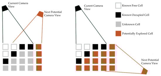
Figure 1.
Illustration of the NBV problem.
Many existing methods are designed for high-resolution object scanning and rely on techniques like volumetric ray-casting to evaluate information gain. Other approaches, such as frontier-based exploration developed for mobile robots, do not easily translate to the kinematic constraints and limited reach of a fixed-base manipulator. Finally, while powerful, recent learning-based methods often require extensive, object-specific training data and can struggle to generalize to novel workcell layouts, a significant drawback in flexible manufacturing. These general limitations of existing methods—high computational cost, platform incompatibility, and a lack of on-the-fly adaptability—hinder their practical deployment in dynamic industrial settings.
To address these challenges, this paper proposes a novel NBV method specifically designed for the complete and efficient exploration of a robotic arm’s entire, initially unknown workspace. The main contribution of this work is a holistic framework that integrates several key features. We introduce a computationally efficient information gain metric that relies on a fast, collision-based assessment, avoiding the high cost of traditional ray-casting. This is paired with a lightweight potential field method to generate and orient candidate views from the frontiers of the known space, effectively directing the robot while respecting its kinematics. These components are unified within a single, tunable fitness function that balances the critical trade-off between maximizing information gain and minimizing motion cost. The robustness and practical viability of this integrated approach are demonstrated through rigorous testing in diverse simulated environments and, crucially, through validation on a physical industrial robot.
In all setups, our method successfully explores the majority of the robot’s workspace, providing a practical solution for enabling advanced automation in modern manufacturing.
2. Related Works
The Next-Best-View (NBV) problem has evolved into a rich family of techniques that balance information gain, motion cost and real-time feasibility across mobile and fixed-base platforms. In the context of Industry 4.0 work-cells—where fixtures, workpieces and even human co-workers may change between shifts—the demand has shifted from object-centric scanning to workspace-centric exploration able to cope with incomplete or outdated CAD data. The paragraphs below review this progression and position our potential-field, collision-based planner with respect to current state-of-the-art techniques.
Early NBV research focused on volumetric information gain computed by ray-casting or frontier enumeration. Classical frontier-RRT planners for mobile robots [] already demonstrated good coverage but struggled with the exponential growth of candidate evaluations in cluttered 3-D scenes. Subsequent benchmarks, such as Delmerico et al. [], quantified how various visibility-likelihood models affect reconstruction accuracy, paving the way for more selective candidate generation. Recent “optimal frontier’’ extensions reduce this computational burden by evaluating only dynamically-maintained frontier sets; Lu et al.’s sparse RRG approach, for example, halves gain-evaluation time while preserving coverage accuracy [].
Information-theoretic formulations remain dominant for manipulators dedicated to high-resolution object modeling. Two-stage planners [] that first choose coarse viewpoints and then refine them locally or that adapt voxel size through multi-resolution max-flow optimization [] offer excellent surface completeness, yet they still rely on millions of rays per NBV cycle. When occlusions are severe, shadow-casting NBV [] provides a GPU-friendly alternative, but at the expense of extra memory for visibility maps. Our method departs from this family by replacing ray-casting with a fast collision-set test on the live octomap.
Utility-balanced planners explicitly mix exploration reward with kinematic or energetic costs. Environment-guided exploration [] augments frontier gain with time-and-effort penalties and Liu et al. optimize frontier costs in real time using local map statistics []. We adopt the same philosophy but cast distance, rotation change, and collision-derived gain into a single scalar fitness; the ablation study in Section 4 shows that the unequal weighting of these terms yields shorter paths than the uniform weighting traditionally assumed in utility literature.
Learning-based NBV has gained momentum because neural policies can amortize the cost of ray-casting across training episodes. BENBV-Net learns a boundary-exploration policy that generalizes across objects [], Monica & Aleotti predict gain maps with a lightweight CNN so that only the most promising voxels are evaluated online [], and Zeng et al. train a deep-RL agent that maximizes fruit visibility in agricultural orchards []. While these approaches excel once training data exist, their reliance on object or environment priors limits applicability in brown-field factories where layouts change daily. Our training-free strategy therefore complements learning-based NBV by offering a drop-in solution for cells that are re-configured on the fly.
Industry-oriented surveys emphasize that up-to-date environment models are essential for collision-free motion planning, scheduling and, digital-twin synchronization [], the recent synthesis of active mapping and robot exploration trends reaches the same conclusion []. Yet most NBV studies still assume static or slowly changing scenes. By computing information gain from current collision geometry rather than pre-existing CAD, our planner inherently handles movable tooling and work-pieces—an aspect under-served in frontier or learning-based work that bakes static occupancy into the reward.
Finally, papers that blur the boundary between manipulation and mobility deserve mention. Efficient topological-map exploration for UAVs [] and incrementally-built PRM for mobile manipulators [] demonstrate how global coverage benefits from hierarchically structured maps. The potential-field edge detector we employ serves a similar purpose for fixed-base arms: it provides a lightweight surrogate frontier aligned with manipulator kinematics without the overhead of maintaining multi-layer graphs.
Taken together, the literature shows three distinct trends—ray-casting information theory, multi-objective utility, and data-driven learning—each excelling in specific metrics. Our contribution resides at the intersection, it keeps the interpretability and task-agnosticism of classical information gain, inherits the cost awareness of utility-based selection, and brings real-time responsiveness akin to light CNN surrogates, all without off-line training or CAD assumptions.
3. Our Implementation
The NBV methods implemented on the robotic arm are mainly aimed at the 3D reconstruction of objects. The NBV method we propose is designed to explore the entire environment around the robot. Unfortunately, it is impossible to search a completely unknown environment with a camera located on the flange. Hence, an initial collision-free trajectory is carried out to obtain basic information about the environment.
The problem of searching the environment is divided into two processes, namely mapping and planning. This paper is primarily focused on planning and NBV methods; therefore, the mapping process is not described in detail. The overall process, detailed in Algorithm 1, operates in a closed loop: the robot moves to a selected view, acquires sensor data, updates its 3D octomap of the environment, and then uses this new map information to plan the next best view. The planning process consists of combining the proposed NBV method with the planning of the robot’s trajectories to the proposed pose from NBV. Individual planning components are designed to be easily swapped for other implementations.
| Algorithm 1 Basics steps of NBV |
|
3.1. Environment Representation
The robot consists of connected links with a known kinematic structure, where joint rotations define its state for trajectory planning. The environment is represented as an octomap [], a 3D occupancy grid that efficiently models free and occupied space, with cells classified as unknown, occupied, free, and overlaid. Initially set to unknown, cells are updated based on visual data. To prevent the robot from erroneously perceiving its own body as an obstacle, standard self-filtering mechanisms are employed when integrating sensor data into the octomap. Additionally, to ensure valid initial path planning, octomap cells corresponding to the robot’s volume at its initial pose are explicitly marked as free space.
3.2. Initial Phase
In this phase, initial information about the environment is acquired through minimal motion limited to the fifth and sixth joints, altering only the pose of the flange-mounted camera. This ensures that the rest of the robotic arm remains stationary and does not interact with the unknown surroundings. By varying the camera orientation, the robot incrementally uncovers regions that were initially out of view due to its mounting configuration and kinematic structure. The only assumption is the absence of obstacles within a defined minimum radius around the camera.
3.3. Candidate Generator
In the first step of NBV, candidates for camera poses that could potentially scan new information about the environment are generated. Our proposed method is based on finding edges between known and unknown environment and utilizing the potential field []. There are numerous methods of edge detection in a grid map, in an image, or in a point cloud, summarized in []. For the sake of simplicity, the edges are detected by sequentially searching all cells of the map and verifying the states of adjacent cells. A cell is considered to be on an edge if it meets a required ratio of unknown to known neighboring cells. Its position is then referred to as . This ratio will be adjustable as a parameter of the algorithm. It would not be efficient to search all cells of the map in each iteration; therefore, the edges are only searched in the new altered states. The candidate’s direction is determined by the potential field, in which the known space is the repulsive force and the unknown space acts as an attractive force . The closer the cell is to the cell lying on the detected edge, the more impact it has. Therefore, the elements of vectors and have the following values:
where , , and are the coordinates of the adjacent cell relative to the cell lying at the detected edge and is the maximum effective distance between the cells. From the equations, we can conclude that the closer cell has a bigger effect than the distant cell. The resultant force is then sum of all the forces from all the adjacent cells (Equation (4)), where is the number of unknown cells that act by an attractive force and is the number of known cells that act by a repulsive force.
A graphical demonstration of determining the candidate’s direction is shown in Figure 2, where the black cell represents the cell lying on the detected edge between the known and unknown environment. White cells represent the known environment and act with a repulsive force, while gray cells represent the unknown environment and act with an attractive force. The maximum effective distance is set to the value of two adjacent cells.
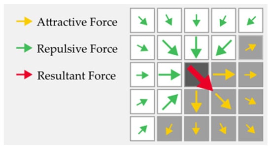
Figure 2.
Selection of candidate direction using the potential field.
The position of the candidate is determined by the cell lying on the detected edge between the environments, but due to the minimum scanning distance of the camera, the position of the candidate must be shifted by a constant value in the z-axis so that the camera can also capture this edge.
3.4. Filters
The generated set of candidates may be unnecessarily large, slowing down the NBV process. Discarding unpromising or redundant candidate views prior to computationally expensive evaluation is a common strategy to enhance NBV efficiency []. Such filtering techniques often rely on various criteria, including evaluating the expected information gain against certain thresholds or metrics [,] assessing visibility and required overlap, or reducing spatial redundancy among candidates. The aim of filtering stages in our method is to remove possible clusters of candidates and those candidates pointing primarily towards already explored space. The order of our filters is chosen such that computationally cheaper checks are performed first, reducing the set processed by slower evaluations.
- (1)
- Out of Range Filter (ORF)
The first filter removes the candidates that are out of reach of the robot by calculating the Euclidean distance (5) from the robot base:
- (2)
- Position Threshold Filter (PTF)
The second filter, the Position Threshold Filter (PTF), aims to prune the set of new candidates by removing those that are redundant. A candidate is considered redundant if it is too close in both position and orientation to a candidate that has already been accepted. This prevents the planner from evaluating dense clusters of near-identical views.
To do this efficiently, we maintain a set of accepted, non-redundant candidates. For each new candidate, we check if it lies within a distance threshold of any accepted candidate. If it does, we also check if its orientation is significantly different. A new candidate is only accepted if it is either far away from all existing candidates or, if it is nearby, it offers a sufficiently novel orientation. To accelerate the spatial proximity search, the positions of accepted candidates are stored in a k-d tree [], which allows for near-constant time lookups. This process is detailed in Algorithm 2.
| Algorithm 2 Position Threshold Filter |
|
The computations for , , and are referenced in [].
- (3)
- Information gain filter (IGF)
A filter based on information gain can be used at the final stage to assess whether a candidate can explore enough unknown space.
The information gain expresses the ratio of the known to the unknown environment in a given camera view. A greater value means that the candidate can potentially search more space. The calculation of the information gain in this proposed NBV algorithm is based on collision detection []. The intersection of the scanned space with an unknown environment is calculated. The process of collision detection is shown in Figure 3, where the green arrow represents the camera view, the potentially scanned space is indicated in yellow, the gray cells represent the unknown space, and the white cells represent the searched space. The collisions are marked red.

Figure 3.
Illustration of the information gain calculation.
Let be a number of cells in scanned space and is the maximum possible number of scanned cells, that could lie in this space, then the information gain is denoted as a ratio between and :
- (4)
- Next Best View selection
The next phase of the NBV method is to sort the filtered set of candidates according to a fitness function. The fitness function considers the information gain while minimizing the distance traveled by the robot and the rotations of the camera. Let us define the fitness function of the distance traveled as follows:
where is the Euclidean distance in the robot’s frame between the current position of the camera and the position of the camera in the candidate The constant represents the maximum range of the robot, which must be multiplied by two, since the candidate’s position can be in the interval from − to The value of the fitness function is greater if the Euclidean distance is smaller. For the rotation fitness function, we will write the following:
where denotes the difference in orientation between the current orientation and the orientation in the candidate. Again, the smaller the change in orientation, the greater the fitness function value. The best candidate is the one with the greatest value of the fitness function, which is defined as the combination of the Equations (6)–(8):
3.5. Termination Criteria
The proposed NBV exploration process ceases when specific criteria are met, indicating either completion or the inability to make further progress. Primarily, termination occurs when the algorithm fails to determine a valid next best view. This situation arises if there are no more suitable candidates generated, all candidates are discarded in the filtering stage or all filtered candidates subsequently fail necessary validation steps, such as inverse kinematics solvability or collision-free path planning, preventing the robot from reaching any potential view.
Additionally, the exploration can be configured to terminate when the ratio of the explored volume to the total target workspace volume exceeds a predefined threshold (e.g., 95%), signifying sufficient coverage has been achieved, even if some unexplored frontiers might remain. This ensures the process concludes either upon comprehensive mapping according to the planner’s logic or when a user-defined coverage goal is met.
4. Experiments
The aim of these experiments is to systematically evaluate the functionality of the proposed method and understand the effect of the fitness function’s weights on exploration performance. We designed our experiments as an ablation study to isolate the impact of each core criterion. For the first experiment, we tested extremal configurations where one weight is set to 1 and the others to 0 to observe the behavior of each criterion in isolation. We also tested a balanced configuration where all criteria are weighted equally. For subsequent experiments in more complex environments, we tested combinations informed by these initial results.
The results were obtained in both simulated and real-world environments. The simulations were conducted using Gazebo (v11.15.1), while the physical experiment utilized an ABB IRB 4600 robotic arm (ABB Ltd., Zürich, Switzerland). Both the ABB IRB 4600 (used in experiments 1, 2, and 4) and the ABB IRB 2400 (used in experiment 3) were controlled via ROS (noetic). In all experiments, a Kinect v2 depth camera (Microsoft Corp., Redmond, WA, USA), with a maximum range of 5 m, was mounted on the robot flange to provide visual input. The simulated camera model was configured to match the specifications of its real-world counterpart.
The arm trajectory was planned by the RRTConnect [] algorithm and the candidate’s position was transformed into the robot’s frame by the inverse kinematics IKFast []. If the inverse kinematics calculation or the trajectory planning failed, the next best candidate was chosen.
To generate a trajectory, the candidate pose was first converted into multiple invariant orientations around the Z-axis. For each pose variant, the inverse kinematics solver attempted to find all valid joint configurations using MoveIt’s IK interface with collision checking from the planning scene. The evaluation took place in four different environments with different complexities.
The experimental scenarios were designed to reflect typical industrial applications and to incrementally increase in complexity. Our first experiment modeled a common use-case where a robot started in a safe, open ‘home’ position. Subsequent experiments introduced more clutter and confinement to systematically test the planner’s limits, culminating in a final validation on a physical robotic platform.
4.1. First Experiment
The first simulation environment was considered trivial because after the initial phase, only about 30% of the unknown environment remained, as illustrated in Figure 4. On the left, a simulation environment is displayed, where red zones represent overlaid places that the camera cannot capture at the initial phase. On the right is the state of the environment after the initial phase, which contains about 30% of the unknown environment. The cubes of an octree (with a color scale by height) depict a combination of unknown and occupied space. The trajectory planning algorithm considers this octal tree as a collision object. By gradually scanning the environment, the octal tree is reduced and at last, only occupied and unreachable cells should remain.
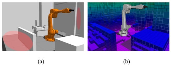
Figure 4.
(a) The first experiment setup; (b) the occupied and unknown space after the initial phase.
The elements of the fitness function are decomposed so that the influence of individual elements can be clearly seen. In three separate measurements, the maximum weight 1 for the chosen element was set, while the weights of the others were 0. The fourth measurement consisted of equally set weights. The experiment was thus be carried out in four measurements:
- IG1_T0_R0—Information gain weight 1, others 0;
- IG0_T1_R0—Weight of the distance of the candidate from the current camera position 1, others 0;
- IG0_T0_R1—Weight of the rotation difference between candidate and current camera position 1, others 0;
- IG1_T1_R1—All weights equal to 1.
The total decrease in the value of the fitness function with respect to the selected candidates is shown in the graph in Figure 5. The value of IG1_T0_R0 is significantly lower than in the case of other experiments. Since the workspace of the robot is limited (depending on the robot used) and the range of the scanner is up to 5 m, it is impossible to achieve maximum information gain. The highest information gain value is only around 0.3; however, the distance fitness function can have a significantly greater impact, as the worst distance can be twice the robot’s, but usually, the positions of the candidates are significantly closer. Therefore, in the IG1_T1_R1 measurement, information gain was less preferred. It is advisable to compensate for this imbalance by unevenly distributing the weights.
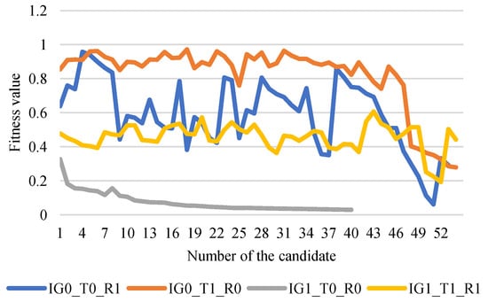
Figure 5.
The fitness value with respect to the selected candidate.
Figure 6 illustrates the NBV algorithm’s progress across iterations. The results indicate that IG1_T0_R0 achieves the fastest convergence to the total scanned space.
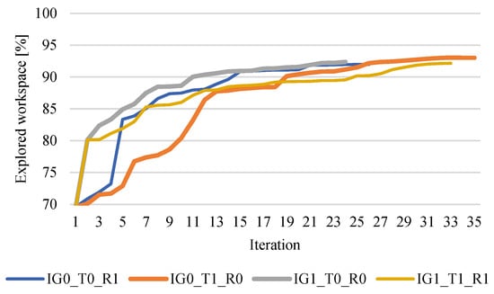
Figure 6.
Explored volume of the workspace in each iteration in the first experiment.
Although IG1_T0_R0 searched the space in fewer iterations, this does not guarantee that the total distance traveled is the shortest, which can significantly impact the total duration of exploration. The total length of the trajectory is evaluated using criteria listed below:
- Joint Distance (JD): This metric calculates the sum of the absolute angular distance traveled by each of the robot’s joints throughout the entire trajectory. A lower JD signifies less overall joint movement.
- Control Pseudo Cost (CPC): This is a weighted version of JD, where the movement of larger joints (closer to the robot base) is penalized more heavily than the movement of smaller joints. It provides a more realistic estimate of energy consumption.
- Cartesian Distance (CD): This metric measures the total distance traveled by the robot’s end-effector in 3D space.
- Orientation Change (OC): This calculates the sum of the absolute angular changes in the end-effector’s orientation between consecutive points in the trajectory. It is a key indicator of rotational smoothness; a lower OC suggests fewer and less abrupt reorientations of the tool.
- Robot Displacement Metric (RDM): The RDM is the sum of the Cartesian distances traveled by the center of mass of each of the robot’s links. It provides the most comprehensive measure of the total motion of the entire robot structure, not just the end-effector.
Criteria are presented in detail in our previous research Evaluation Criteria for Trajectories of Robotic Arms published in [].
The resulting total sums of the criteria are shown in Table 1, where the color of each row matches the corresponding plots in Figure 5 and Figure 6 The best results are marked in bold. From the results, it can be seen that the IG1_T0_R0 experiment searched the space in the fewest iterations but was the longest in terms of all other criteria. Overall, the distribution of the weights of the fitness function in IG1_T1_R1 can be evaluated as the most effective because it quickly converged to the solution and from the point of view of the traveled distance, it achieved comparable results to the experiments of IG0_T1_R0, where the shortest distance to the candidates was preferred. In the case of IG0_T0_R1, where the minimization of camera rotation is preferred, an unexpected behavior occurs: the traveled rotation (criterion OC) is the worst. It is caused by the fact that the chosen candidate has the lowest difference in orientation, but it is located far away from the current pose and the planned path may be complicated. Therefore, we do not recommend that using the high preference of the rotation minimization or path planner should consider rotation constraints, e.g., our extension of STOMP algorithm [], which is able to minimize tool point rotation in a trajectory.

Table 1.
Sums of criteria values computed by [] in the first experiment.
4.2. Second Experiment
The second environment is more complicated because in the initial phase, the camera view is limited by the walls around it, as illustrated in Figure 7. Therefore, after the initial phase, more than 80% of the unknown space remains. The NBV algorithm should search these locations by gradually acquiring new information about the environment.
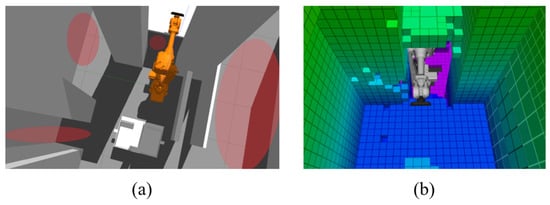
Figure 7.
(a) The second experiment setup; (b) the occupied and unknown space after the initial phase.
For this more complex environment, we refine our selection of weight configurations based on the findings from the first experiment. The extremal configurations IG1_T0_R0 (pure information gain) and IG0_T1_R0 (pure distance minimization) are retained to serve as baselines. The IG0_T0_R1 (pure rotation) and IG1_T1_R1 (equal weights) configurations are omitted, as the first experiment demonstrated their suboptimal performance.
Based on our initial findings, we hypothesized that a successful strategy must balance the aggressive exploration of information gain with the efficiency of distance minimization. Therefore, we introduce two new configurations to test this trade-off: IG1_T05_R01 and IG1_T025_R01. These configurations heavily prioritize information gain but add a small, non-zero weight for and rotation to act as penalties for overly long or complex movements. This allows us to investigate whether a small travel cost consideration can temper the otherwise greedy nature of an information-gain-only approach.
The results shown in Figure 8 meet the expectations. Again, the more the information gain is preferred, the faster the space is searched, but there is an increased risk of getting trapped in the local maximum. On the other hand, the more distance minimization is preferred, the more iterations the algorithm requires, but the total distance traveled is shortened, as shown in Table 2. The best results are marked in bold.
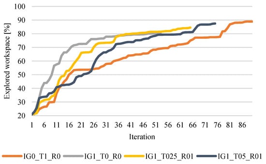
Figure 8.
The explored volume of the workspace in each iteration in the second experiment.
Table 2.
Sums of criteria values computed by [] in the second experiment.
4.3. Third Experiment
The third environment represents a real-world application in which the robot is mounted on a stand to reach the conveyor during a pick-and-place operation. The conveyor is located inside a robotic safety cage, as shown in Figure 9. Unlike the previous experiments, this setup utilizes the ABB IRB 2400 robot. The same fitness function weight configurations as in the second experiment were used, specifically, IG1_T0_R0, IG0_T1_R0, IG1_T05_R01, and IG1_T025_R01.
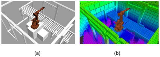
Figure 9.
(a) The third experiment setup; (b) the occupied and unknown space after the exploration phase.
The exploration progresses over time, as shown in Figure 10, and confirms the findings from the second experiment. The exploration phase began when approximately 60% of the space had already been explored in the initial phase, leaving the NBV algorithm responsible for exploring the remaining 40%. Although the configuration maximizing the T weight (with other weights set to zero) initially showed the fastest growth, its progress slowed after a few iterations and ultimately required the most iterations to complete the exploration until the stop condition was hit.
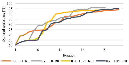
Figure 10.
The explored volume of the workspace in each iteration in the third experiment.
Table 3 summarizes the performance of each configuration in the third experiment. Although IG1_T0_R0 searched space in the fewest iterations, it also produced the highest values across all cost-related criteria, indicating inefficient motion. In contrast, IG0_T1_R0 and IG1_T025_R01 achieved significantly lower values in joint and Cartesian distances, orientation change, and overall robot displacement, suggesting more efficient and smoother trajectories. Notably, IG1_T025_R01 maintained comparable exploration performance while minimizing motion costs, making it a well-balanced option. The best results are highlighted in bold, while row colors align with the data plots in Figure 10.
Table 3.
Sums of criteria values computed by [] in the third experiment.
4.4. Fourth Experiment
To demonstrate the practical applicability of our proposed NBV method, a final experiment was conducted under laboratory conditions at the National Centre of Robotics in Slovakia. The setup was designed to partially replicate a real industrial manufacturing cell, featuring key components, such as a conveyor belt, an automatic tool changer, and part bins, to create a realistically complex and cluttered environment. This experiment served as a proof-of-concept to validate that the planner, developed and tested in simulation, can successfully guide a real robot to explore a complex, initially unknown environment.
Based on the simulation results, which identified it as a well-balanced and efficient configuration, the fitness function weights were set to IG1_T025_R01. To prioritize rapid demonstration over high-fidelity mapping, the octomap voxel size was set to a coarse 12.5 cm. While this large voxel size risks missing smaller obstacles, it was deemed sufficient for proving the core functionality of the exploration algorithm on real hardware.
A significant challenge in the real-world setup was the lack of hardware synchronization between the robot controller and the Kinect v2 camera. To ensure stable point cloud acquisition, the robot was programmed to pause at each planned viewpoint before triggering a scan and updating the map. Due to the absence of a ground-truth model of the workcell, the exploration could not be terminated based on a percentage of volume explored. Instead, the process was terminated manually after the robot had successfully mapped the primary operational areas.
The exploration process was successfully executed on the real hardware. The robot first performed an initial scanning phase of 21 views to build a foundational map of its immediate surroundings. Following this, the NBV exploration algorithm took over, autonomously generating and executing trajectories for another 16 views.
Figure 11 The explored volume of the workspace during the initial phase in the fourth experiment shows the state of the octomap after the 15/21 scans in the initial phase. While the robot’s immediate vicinity is mapped, significant portions of the environment remain unknown, particularly the area behind the conveyor belt and the upper regions of the workcell.
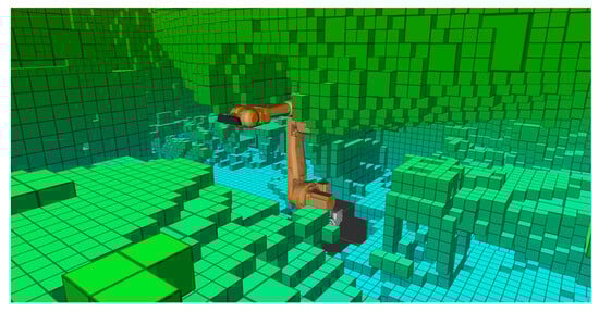
Figure 11.
The explored volume of the workspace during the initial phase in the fourth experiment.
Figure 12 displays the final map after the 16-view exploration phase. The algorithm successfully guided the robot to explore these previously occluded areas, clearly mapping the full conveyor system, a nearby parts stand with totes, and the tool holders located behind the robot’s initial position. It is important to note that the physical tool changer, mounted between the robot flange and the camera, was not explicitly present in the simulation due to the lack of a 3D model. However, its physical dimensions were accounted for by applying a corresponding static transformation to the sensor frame in simulation, ensuring that the robot’s reach and the camera’s viewpoint accurately reflected the real hardware.
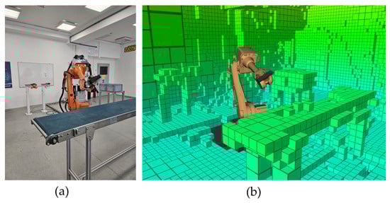
Figure 12.
(a) The fourth experiment setup; (b) the occupied and unknown space after the exploration phase.
Overall, the experiment successfully demonstrated the suitability of the proposed NBV algorithm for real-world application. The robot navigated a complex environment, autonomously identifying and scanning unknown regions to build a comprehensive map. The primary limitation observed was the coarse map resolution due to the large voxel size. Future work should focus on implementing hardware synchronization to eliminate pauses, using a smaller voxel size for higher-fidelity mapping, and performing a more rigorous calibration of the camera’s extrinsic parameters to further improve accuracy. Despite these areas for improvement, the results confirm that the proposed method is a viable foundation for autonomous workspace exploration in real industrial settings.
5. Discussion
The majority of Next-Best-View methods applied to industrial robots with hand-eye camera systems typically focus on 3D object modeling within a localized robot workspace. In contrast, our proposed NBV approach provides a methodology for exploring the entire reachable workspace of the robotic arm. The resulting comprehensive environment model is a key enabler for Industry 4.0 applications, holding significant potential for advanced industrial scenarios requiring detailed scene understanding. These include the development of accurate digital twins for offline programming and simulation, enhanced collision-free path planning for dynamic manufacturing environments, and fostering safer human-robot collaboration through complete workspace awareness.
The theoretical novelty of our approach is rooted in its combination of a potential field for guiding view selection with an information gain metric based on collision detection. In contrast to the common volumetric NBV methods, which use ray-casting for information gain estimation, our NBV uses a collision check between the view frustum and unknown voxels. This provides a computationally efficient proxy for information gain that is well-suited for on-robot deployment.
Through a series of three distinct simulation experiments and a final real-world validation, including scenarios with varying environmental complexity and one featuring a realistic robotic workcell, we demonstrated the proposed method’s functionality. The experiments systematically studied the impact of different weightings in the fitness function. Based on these results, we can conclude the following behaviors, which are summarized in Table 4.
Table 4.
Summary of weighting strategy characteristics.
Prioritizing information gain generally leads to a faster volumetric search of the space. However, this can result in candidate views being dispersed far from the current robot pose. In complex environments, this increases the risk of trajectory planning failures or encountering unreachable candidates, which might be prematurely discarded but could become accessible later from a different vantage point. This challenge is more pronounced when a large proportion of the environment remains unknown after the initial exploration phase.
Conversely, emphasizing the minimization of travel distances (translation and rotation) tends to select closer candidates. This facilitates simpler trajectory planning, reduces failures, and significantly improves the overall path quality and total distance traveled. The trade-off is a potential increase in the number of iterations required, especially in simpler environments.
A high preference for minimizing rotational differences between the current and candidate views did not consistently yield better trajectory quality or lower total orientation changes (OC criterion). This is because a candidate with minimal orientation change might be distant, leading to complex paths with more frequent reorientations. However, a modest weight for rotation minimization can be beneficial, acting as a tie-breaker between candidates otherwise similarly rated by information gain and travel distance.
While our approach demonstrates a robust framework for workspace exploration, its reliance on fixed fitness function weights and a simple failure-handling mechanism highlights clear directions for future enhancement. As our study shows, the optimal balance between exploration and efficiency can change during the mapping process. This suggests that the most significant future work lies in developing an adaptive weighting scheme. Such a system could dynamically adjust the fitness function, for instance, by prioritizing distance minimization when the map is sparse and then shifting focus to information gain to fill in smaller, remaining gaps as the workspace becomes better known.
Furthermore, the current strategy for handling trajectory planning failures could be made more sophisticated. Future improvements could include re-attempting previously failed candidates from new robot poses or incorporating a penalty into the fitness function based on the historical frequency of planning failures for a given region. These advancements would lead to a more intelligent and resilient exploration planner.
6. Conclusions
This paper introduced a novel Next-Best-View (NBV) approach designed for the comprehensive exploration of a robotic arm’s entire reachable workspace, a departure from traditional object-centric modeling methods. Our method leverages a potential field to guide view selection and a computationally efficient collision-based metric to estimate information gain. Through a series of three simulation experiments and a final real-world validation, we have demonstrated its effectiveness and systematically analyzed the trade-offs between exploration speed and path efficiency.
The key findings indicate that prioritizing information gain accelerates volumetric coverage at the cost of path efficiency, while emphasizing travel distance minimization results in more reliable and shorter trajectories, albeit at a slower exploration pace. Our validation on a physical robotic platform confirmed that a balanced strategy, which moderately penalizes travel cost, provides a robust and practical solution for exploring complex, real-world environments.
This work advances the field by providing a practical and computationally lightweight framework for creating comprehensive, on-demand 3D models of industrial workcells. Such models are a critical enabler for Industry 4.0 applications, including the development of accurate digital twins, enhancing collision-free path planning in dynamic settings, and fostering safer human-robot collaboration through complete workspace awareness.
Despite its success, this study has limitations. The proposed method was validated primarily in static environments, and its performance relies on a fixed-weight fitness function, which may not be optimal for all stages of exploration. Furthermore, the real-world implementation, which required the robot to pause for each scan, highlighted a key area for advancement: enabling continuous mapping while the robot is in motion. Achieving this would require robust synchronization between the robot’s state estimation and the camera’s data acquisition to handle motion blur and accurately register point clouds in real-time. Finally, the coarse map resolution used in our validation underscores the need for finer voxel sizes when detailed object reconstruction is required.
Future work will focus on addressing these limitations. Our primary goal is to develop an adaptive weighting scheme for the fitness function, allowing the robot to dynamically shift its priorities from efficient travel to detailed scanning as the map becomes more complete. We will also explore more sophisticated strategies for handling trajectory planning failures, such as re-attempting failed candidates or penalizing historically difficult regions. Additionally, we plan to extend the framework to handle dynamic environments by detecting and re-scanning areas with changed occupancy. Finally, we will investigate parallelizing the mapping and planning processes to enable real-time 3D reconstruction synchronized with robot motion, with the goal of migrating the entire system to ROS 2 to leverage its advancements in real-time capabilities and long-term support.
Author Contributions
Conceptualization, M.D. (Michal Dobiš), M.D. (Martin Dekan) and F.D.; methodology, M.D. (Michal Dobiš), J.I., M.D. (Martin Dekan) and A.B.; software, M.D. (Michal Dobiš) and J.I.; validation, M.D. (Michal Dobiš), J.I. and R.M.; formal analysis, M.D. (Michal Dobiš), J.I., A.B. and R.M.; investigation, M.D. (Michal Dobiš) and M.D. (Martin Dekan); resources, M.D. (Michal Dobiš), J.I., M.D. (Martin Dekan) and R.M.; data curation, M.D. (Michal Dobiš) and R.M.; writing—original draft preparation, M.D. (Michal Dobiš) and R.M.; writing—review and editing, M.D. (Michal Dobiš) and J.I.; visualization, M.D. (Michal Dobiš), J.I. and R.M.; supervision, M.D. (Martin Dekan) and F.D.; project administration, F.D. and A.B.; funding acquisition, F.D. and A.B.; All authors have read and agreed to the published version of the manuscript.
Funding
KEGA 036STU-4/2024 supported this work. Operational Program Integrated Infrastructure created this publication for the project: “Digitalization of robotic workplace for intelligent welding,” code ITMS2014+: 313012S686, and it is co-sponsored by the European Regional Development Fund.
Data Availability Statement
The raw data supporting the conclusions of this article will be made available by the authors on request.
Conflicts of Interest
The authors declare no conflict of interest.
Abbreviations
The following abbreviations are used in this manuscript:
| NBV | Next Best View |
| FLANN | Fast Library for Approximate Nearest Neighbors |
| PCL | Point Cloud Library |
| JD | Joint Distance |
| CPC | Control Pseudo Cost |
| CD | Cartesian Distance |
| OC | Orientation Change |
| RDM | Robot Displacement Metric |
References
- Kang, Z.; Yang, J.; Yang, Z.; Cheng, S. Review of Techniques for 3D Reconstruction of Indoor Environments. ISPRS Int. J. Geo-Inf. 2020, 9, 330. [Google Scholar] [CrossRef]
- Tian, X.; Liu, R.; Wang, Z.; Ma, J. High Quality 3D Reconstruction Based on Fusion of Polarization Imaging and Binocular Stereo Vision. Inf. Fusion 2022, 77, 19–28. [Google Scholar] [CrossRef]
- Scott, W.R.; Roth, G.; Rivest, J.-F. View Planning for Automated Three-Dimensional Object Reconstruction and Inspection. ACM Comput. Surv. 2003, 35, 64–96. [Google Scholar] [CrossRef]
- Umari, H.; Mukhopadhyay, S. Autonomous Robotic Exploration Based on Multiple Rapidly-Exploring Randomized Trees. In Proceedings of the 2017 IEEE/RSJ International Conference on Intelligent Robots and Systems, Vancouver, BC, Canada, 24–28 September 2017. [Google Scholar]
- Delmerico, J.; Isler, S.; Sabzevari, R.; Scaramuzza, D. A comparison of volumetric information gain metrics for active 3D object reconstruction. Auton. Robot. 2017, 42, 197–208. [Google Scholar] [CrossRef]
- Lu, L.; De Luca, A.; Muratore, L.; Tsagarakis, N.G. An optimal frontier enhanced “next best view” planner for autonomous exploration. In Proceedings of the 2022 IEEE-RAS 21st International Conference on Humanoid Robots, Ginowan, Japan, 28–30 November 2022; pp. 397–404. [Google Scholar]
- Meng, Z.; Qin, H.; Chen, Z.; Chen, X.; Sun, H.; Lin, F.; Ang, M.H. A two-stage optimized next-view planning framework for 3-D unknown environment exploration, and structural reconstruction. IEEE Robot. Autom. Lett. 2017, 2, 1680–1687. [Google Scholar] [CrossRef]
- Pan, S.; Wei, H. A global max-flow-based multi-resolution next-best-view method for reconstruction of 3d unknown objects. IEEE Robot. Autom. Lett. 2021, 7, 714–721. [Google Scholar] [CrossRef]
- Batinovic, A.; Ivanovic, A.; Petrovic, T.; Bogdan, S. A shadowcasting-based next-best-view planner for autonomous 3D exploration. IEEE Robot. Autom. Lett. 2022, 7, 2969–2976. [Google Scholar] [CrossRef]
- Butters, D.; Jonasson, E.T.; Stuart-Smith, R.; Pawar, V.M. Efficient environment guided approach for exploration of complex environments. In Proceedings of the 2019 IEEE/RSJ International Conference on Intelligent Robots and Systems (IROS), Macau, China, 3–8 November 2019; pp. 929–934. [Google Scholar]
- Liu, C.; Zhang, D.; Liu, W.; Sui, X.; Huang, Y.; Ma, X.; Yang, X.; Wang, X. Enhancing autonomous exploration for robotics via real time map optimization and improved frontier costs. Sci. Rep. 2025, 15, 12261. [Google Scholar] [CrossRef] [PubMed]
- Li, L.; Zhang, X. Boundary Exploration of Next Best View Policy in 3D Robotic Scanning. arXiv 2024, arXiv:2412.10444. [Google Scholar]
- Monica, R.; Aleotti, J. A probabilistic next best view planner for depth cameras based on deep learning. IEEE Robot. Autom. Lett. 2021, 6, 3529–3536. [Google Scholar] [CrossRef]
- Zeng, X.; Zaenker, T.; Bennewitz, M. Deep reinforcement learning for next-best-view planning in agricultural applications. In Proceedings of the 2022 International Conference on Robotics and Automation (ICRA), Philadelphia, PA, USA, 23–27 May 2022; pp. 2323–2329. [Google Scholar]
- Lluvia, I.; Lazkano, E.; Ansuategi, A. Active mapping and robot exploration: A survey. Sensors 2021, 21, 2445. [Google Scholar] [CrossRef] [PubMed]
- Wang, C.; Ma, H.; Chenc, W.; Liu, L.; Meng, M.Q.-H. Efficient Autonomous Exploration with Incrementally Built Topological Map in 3-D Environments. IEEE Trans. Instrum. Meas. 2020, 69, 9853–9865. [Google Scholar] [CrossRef]
- Hornung, A.; Wurm, K.M.; Bennewitz, M.; Stachniss, C.; Burgard, W. OctoMap: An efficient probabilistic 3D mapping framework based on octrees. Auton. Robot. 2013, 34, 89–206. [Google Scholar] [CrossRef]
- Uríček, J.; Poppeová a, V.; Zahoranský, R.; Bulej, V.; Kuciak, J.; Durec, P. The Potential Fields Application for Mobile Robots Path Planning. In Proceedings of the 12th International Research/Expert Conference, Instanbul, Turkey; 2008; pp. 505–508. [Google Scholar]
- Bhardwaj, S.; Mittal, A. A Survey on Various Edge Detector Techniques. Procedia Technol. 2012, 4, 220–226. [Google Scholar] [CrossRef]
- Vasquez-Gomez, J.I.; Sucar, L.E.; Murrieta-Cid, R. View/state planning for three-dimensional object reconstruction under uncertainty. Auton. Robot. 2017, 41, 89–109. [Google Scholar] [CrossRef]
- Bentley, J.L. Multidimensional Binary Search Trees Used for Associative Searching. Commun. ACM 1975, 18, 509–517. [Google Scholar] [CrossRef]
- Diebel, J. Representing Attitude: Euler Angles, Unit Quaternions, and Rotation Vectors; Matrix: Sydney, Australia, 2006; pp. 1–35. [Google Scholar]
- Kuffner, J.J.; LaValle, S.M. RRT-Connect: An Efficient Approach to Single-Query Path Planning. In Proceedings of the IEEE International Conference on Robotics and Automation (ICRA), San Francisco, CA, USA, 24–28 April 2000. [Google Scholar]
- Diankov, R. Automated Construction of Robotic Manipulation Programs; Carnegie Mellon University: Pittsburgh, PA, USA, 2010. [Google Scholar]
- Dobiš, M.; Dekan, M.; Sojka, A.; Beňo, P.; Duchoň, F. Cartesian Constrained Stochastic Trajectory Optimization for Motion Planning. Appl. Sci. 2021, 11, 11712. [Google Scholar] [CrossRef]
- Dobiš, M.; Dekan, M.; Beňo, P.; Duchoň, F.; Babinec, A. Evaluation Criteria for Trajectories of Robotic Arms. Robotics 2022, 11, 29. [Google Scholar] [CrossRef]
Disclaimer/Publisher’s Note: The statements, opinions and data contained in all publications are solely those of the individual author(s) and contributor(s) and not of MDPI and/or the editor(s). MDPI and/or the editor(s) disclaim responsibility for any injury to people or property resulting from any ideas, methods, instructions or products referred to in the content. |
© 2025 by the authors. Licensee MDPI, Basel, Switzerland. This article is an open access article distributed under the terms and conditions of the Creative Commons Attribution (CC BY) license (https://creativecommons.org/licenses/by/4.0/).