Featured Application
This work introduces an optimized stacked ensemble model that significantly enhances the accuracy of hourly energy consumption forecasting. This model is particularly valuable for Digital Twin simulations in smart buildings. Its ability to accurately predict energy usage and robustly handle various real-world data challenges (like structural changes, sudden spikes, data quality issues, and appliance malfunctions) makes it an ideal tool for active energy management. Specifically, it can be applied to optimize building energy efficiency by enabling precise adjustments to HVAC systems and lighting, facilitate predictive maintenance of energy-consuming assets by allowing for timely interventions before failures intensify, support sustainable energy management strategies through accurately forecasting savings from efficiency upgrades and tracking their long-term impact, and enhance grid stability via improved demand-side management and real-time anomaly detection. By providing highly reliable and adaptive energy consumption forecasts, this model directly contributes to smarter, more efficient, and sustainable energy management.
Abstract
Modern energy grids, with their regional diversity and complex consumption patterns, require accurate short-term forecasting for operational efficiency and reliability. This study introduces a Stacking Ensemble Forecasting (SEF) framework for multi-region household energy demand, utilizing an optimized stacking ensemble model tuned via Bayesian Optimization to achieve superior predictive accuracy. The framework significantly improved accuracy across Diyarbakır, Istanbul, and Odemis, with a final model demonstrating up to 16.47% RMSE reduction compared to the best baseline models. The final model’s real-world performance was validated through a Simulated Digital Twin (SDT) environment, where scenario-based testing demonstrated its robustness against behavioral changes, data quality issues, and device failures. The proposed SEF-SDT framework offers a generalizable solution for managing diverse regions and consumption profiles, contributing to efficient and sustainable energy management.
1. Introduction
Real-time short-term energy consumption forecasts are critical for the sustainable and efficient operation of modern energy systems [1]. Accurate predictions are vital for balancing energy supply and demand, optimizing power generation schedules, and supporting the integration of renewable energy sources, thereby contributing to significant carbon emission reductions [2,3]. However, the rise of smart grids and diverse regional consumption patterns has introduced significant complexity, pushing traditional forecasting methods to their limits [4]. These conventional statistical methodologies and early Machine Learning (ML) approaches often struggle to capture the high-variance, non-linear, and time-dependent nature of modern energy data, necessitating more robust predictive models [5,6]. While accurate consumption predictions are important for optimizing power generation scheduling, they also maintain supply/demand balance and aid in significant carbon emission reductions [3]. However, the integration of renewable energy sources, with their variable generation characteristics, may introduce uncertainty into power systems. This complexity requires prediction models with higher accuracy and reliability [2]. In this context, there is a need for effective prediction models that are adaptable to regions with diverse geographical and consumption scenarios. While studies on power consumption prediction are common in the literature, the complexity and regional differences of real-world scenarios often restrict the application of the developed models [4]. Traditional statistical methodologies and early Machine Learning (ML) approaches struggle to capture high-variance, non-linear, and time-dependent energy data [4]. Many studies in the literature focus on single regions, limiting their spatial generalization [5]. Consequently, for multi-regional short-term predictions, novel models that combine high accuracy with adaptable structures are needed.
To address these limitations, this paper proposes a novel prediction framework that integrates a Stacking Ensemble architecture and a Simulated Digital Twin (SEF-SDT) environment for multi-region short-term energy consumption forecasting. The proposed model is evaluated using hourly power consumption data from three distinct Turkish regions (Diyarbakır, Istanbul, and Odemis), representing varied household consumption patterns [6]. The developed framework employs several key methodologies, including data preprocessing, optimal base learner selection to create a stacking ensemble via Random Search optimization, and meta-learner hyperparameter tuning using Bayesian Optimization [7]. Moreover, to systematically evaluate the final model’s performance against various real-world scenarios, an SDT environment was implemented for robust stress testing [8].
Energy prediction methodologies are diverse in the literature. While conventional statistical methods (e.g., ARIMA, Exponential Smoothing) and early Machine Learning algorithms (e.g., SVM, ANN) show limited performance when dealing with high-variance and non-linear energy data [9], deep learning methods (e.g., RNN, LSTM, CNN) often provide higher accuracy but bring practical limitations due to large computational costs and demanding data requirements [10].
To overcome these challenges, ensemble techniques (particularly stacking, which combines the outputs of multiple predictive models) have shown promising results in recent years. Stacking effectively reduces both variance and bias by using a meta-learner for optimal integration of base learners to compensate for individual model weaknesses [11]. Consequently, stacking-based ensemble models are increasingly applied as a robust approach for energy consumption prediction in the literature. For instance, Cao et al. achieved reduced error rates in campus building energy predictions using a stacking model optimized with Particle Swarm Optimization (PSO) [12]. Similarly, substantial improvements in MAPE for electrical load prediction were achieved by Luo et al. via a stacking architecture combining CNN-BiLSTM-Attention and XGBoost models [13]. Olu-Ajayi et al. enhanced model adaptability for complex data by developing a stacking approach integrating various ML methods for predicting energy consumption in buildings [14]. Reddy et al. integrated Gradient Boosting and deep learning models with stacking, obtaining higher accuracy in short-term energy predictions [15]. Additionally, predictive performance was improved by Chen and Wang with a stacking model that considered non-linear interactions among various load types in integrated energy systems [16]. The increasing dynamics of modern energy structures highlight the limitations of traditional, passive energy management approaches, which necessitate a demand for responsive forecasting approaches [17]. This need is effectively met by DT systems, which offer dynamic virtual representations of physical energy systems [18,19]. More precisely, DT systems enable comprehensive simulation, scenario analysis, and robust stress testing for improved operational efficiency, failure prediction, and performance optimization. A literature review confirms that simulation is a core principle of DT systems [18], enabling scenario-based analysis of ML models. Particularly, DTs are increasingly applied for energy performance analysis of buildings [20], such as load demand prediction [21] and optimization of HVAC systems [22]. These applications also include enhancing energy efficiency via techniques like Model Predictive Control (MPC) [23]. In particular, this study introduces an SEF-SDT framework designed to support detailed scenario-based prediction, validation, and testing, particularly in contexts where real-time data flow is unavailable.
The integration of DT technologies and stacking ensemble learning enhances energy prediction by utilizing real-world simulation and scenario testing. Despite the individual strengths of DT technologies and stacking ensemble learning, their direct integration within a unified framework remains a research gap. Our literature survey found no prior studies combining stacking ensemble models with a DT simulation environment to assess their efficiency in capturing dynamic real-world energy consumption patterns. In particular, recent studies have introduced stacking-based and hybrid stacking ensemble frameworks for short-term electricity and building load forecasting [24,25], as well as digital-twin-enabled forecasting approaches for power and renewable energy systems [26,27]. However, these works primarily focus on either advanced ensembling or DT-based simulation in isolation. To the best of our knowledge, no study integrates a stacking ensemble with a Simulated Digital Twin (SDT) framework for multi-regional short-term consumption forecasting. This gap motivates our proposed SEF-SDT framework and highlights its novelty. To address this research gap, this paper aims to answer the following question: How can an integrated framework combining stacking ensemble models with a Simulated Digital Twin environment enhance the accuracy and robustness of short-term energy demand forecasting across diverse regions and challenging real-world scenarios?
The key contributions of this work are as follows:
- Novel SEF-SDT Integration: We developed a hybrid framework that integrates a stacking ensemble with simulated DT for robust energy consumption prediction. This framework leverages scenario-based synthetic data generation for real-world performance analysis. The stacking model includes a two-phase design: the optimal base learner subset is obtained via Random Search, and the final meta-learner’s hyperparameters are tuned using Bayesian Optimization. Additionally, we enriched the meta-learner’s input with both base learner predictions in the ensemble and original/lagged features, which differentiates our approach from classic stacking implementations.
- Improved Prediction Performance across Multiple Real-World Datasets: The proposed SEF-SDT model demonstrated enhanced prediction accuracy and reliability in energy consumption prediction, as quantified by the RMSE metric, compared to baseline methods. This improvement was observed across three real-world datasets from household settings in Diyarbakır, Istanbul, and Odemis. This evaluation supports the model’s generalizability and practical applicability across various energy consumption scenarios.
- Systematic Validation through SDT and Enhanced System Reliability: The proposed system’s stability was validated using both historical and scenario-based generated synthetic data from three distinct household locations. The model demonstrated adequate performance and practical applicability for future DT-driven applications, including its adaptability in real-world simulation scenarios such as (i) Behavioral Change, (ii) Data Quality and Reliability, (iii) Device Failure, and (iv) Energy Efficiency Upgrade.
2. Materials and Methods
2.1. Dataset: Description and Data Statistics
In this study, real-world hourly electricity consumption data were utilized from three different residential locations in Turkey: Diyarbakir, Istanbul, and Odemis. These data were obtained from local energy distribution companies. The datasets contain heterogeneous time intervals, which allows for an analysis of the proposed model’s generalization capabilities and consumption dynamics. The time span of each dataset is as follows:
- Diyarbakir: from 8 August 2018, 00:00 to 23 October 2018, 22:00.
- Istanbul: from 4 April 2017, 11:00 to 12 November 2018, 03:00.
- Odemis: from 2 January 2022, 18:00 to 22 October 2023, 18:00.
Table 1 presents the main statistical properties of the three datasets, including sample size, normality test results (%), minimum, quartiles (25th, 50th, 75th), 90th and 95th percentiles, and maximum values. All consumption values are in kilowatt hours (kWh).

Table 1.
Statistical analysis of the raw electricity consumption data for three different regions in Turkey.
Furthermore, Figure 1 shows histograms with Kernel Density Estimation (KDE) curves, which highlight the right-skewed distribution of electricity consumption in all three datasets. While the Istanbul dataset shows the highest skewness, the Diyarbakır and Odemis datasets illustrate more moderate skewness with lower consumption values.
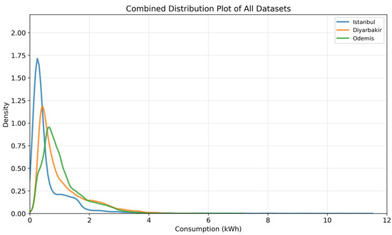
Figure 1.
Histogram analysis of Diyarbakir, Istanbul, and Odemis datasets.
From Table 1, the normality test results (p < 0.001 for all datasets) indicate that all datasets are not normally distributed, which is expected for real-world electricity consumption patterns. These distribution profiles, therefore, highlight the suitability of ensemble methods like stacking for accurately modeling these complex consumption patterns.
2.2. Data Preprocessing
The quality of energy consumption data is critical for prediction models. Therefore, raw data was preprocessed to address issues and prepare it for ML modeling. A series of essential preprocessing steps were applied to ensure data integrity and model robustness.
First, the time series data, which may have missing values, was filled using the median imputation method (Equation (1)) to ensure appropriate data for training. These values are efficiently filled using the median imputation method (Equation (1)) to provide suitable data for training. This method was chosen because the median is a robust statistical measure that is less affected by extreme values or outliers, which helps preserve the original data distribution.
where denotes the energy consumption at a given time , and represents the set of energy values within a specified window around .
Next, outliers, defined as extremely high or low energy consumption values outside typical usage patterns, were addressed. Such anomalies can affect the model during training and negatively impact prediction accuracy. This method was selected because it is a robust, non-parametric approach that does not assume a normal distribution of the data. This makes it highly suitable for real-world energy consumption data, which often contains unpredictable spikes. A value is considered an outlier if it meets one of the conditions in Equation (2).
Here, the Interquartile Range (IQR) is defined as IQR = Q3 − Q1, where Q1 denotes the first quartile (25th percentile) and Q3 the third quartile (75th percentile). Identified outliers were replaced with the corresponding median value to maintain the distribution of datasets.
Finally, Min-Max normalization was used to scale all energy consumption values to a [0, 1] range, thereby balancing feature effects and promoting stable and effective model learning. The normalization is crucial for many ML algorithms, especially those that rely on distance calculations or gradient descent, as it prevents features with larger numerical ranges from disproportionately influencing the model’s training process. Let denote the original energy consumption value at time , while and represent the minimum and maximum values in the dataset, respectively. The normalized value is calculated using Equation (3).
These preprocessing steps are frequently applied in the ML domain in combination to improve data quality for energy prediction tasks.
2.3. Feature Engineering: Construction of Lagged Features
After preprocessing, a time-dependent feature engineering approach was implemented to improve the proposed model’s learning and forecasting capacity. Electricity consumption data exhibits a characteristic called autocorrelation, which means each measurement is affected by past observations. In this context, lagged features are crucial for capturing this temporal dependency, which enables the model to leverage past data for more accurate future predictions. Autocorrelation, or serial correlation, quantifies the linear dependency of a time series with a lagged version of itself over successive time intervals. It is used to identify repeating patterns and cyclical behavior within the data. The significance of these lagged features was rigorously confirmed through an autocorrelation analysis of the three datasets. To model energy consumption at a given time E(t), three specific lagged features were constructed.
- (i)
- Previous Hourly Consumption (E(t − 1)): This feature captures instant and sequential dependencies, and it provides a direct input for short-term forecasting.
- (ii)
- Same-Time Previous Day Consumption (E(t − 24)): This feature captures 24 h patterns, allowing the model to predict repetitive daily variations.
- (iii)
- Averaged Consumption from the Same Hour in the Previous Week (E(t − 168)): This feature captures weekly periodicity, which helps identify weekly patterns and corresponding consumption variations.
By deriving these lagged features, the preprocessed dataset is transformed into an enriched dataset given in Equation (4). This formula mathematically represents the feature engineering process, where the enriched dataset is created by augmenting the original preprocessed dataset with the three constructed lagged features.
This feature engineering phase enabled the model to learn complex repeating patterns, which enhanced forecast accuracy. Construction of lagged features is widely used in energy forecasting literature [28]. The results of the autocorrelation analysis for Istanbul, Diyarbakır, and Odemis confirmed strong and statistically significant correlations at specific lags, with high coefficients reaching up to 0.86. Detailed results and visual presentations of these empirical findings, which validate the temporal dependencies of the consumption data, are located in Section 3.1 of this paper. Furthermore, the effectiveness of these lagged features and their broader correlations with target consumption were also validated by the heatmap analysis presented in the same section.
2.4. The SEF-SDT: A Stacking Ensemble Forecasting via Simulated Digital Twin Approach
As previously stated, the proposed SEF-SDT model consists of two main components: the Simulated Digital Twin (SDT) paradigm [17] and stacking. The SDT paradigm is designed for scenarios without real-time data access and represents a building’s consumption dynamics. This section details the architecture of this integrated model in detail.
To evaluate the model’s performance and obtain constituents of the stacking ensemble, the RMSE was chosen as the primary metric. The SEF model uses a two-layer structure. First, 15 base ML algorithms generate predictions, which are then used as input for the meta-learner. This phase was accomplished through a random search optimization performed on three datasets to determine the optimal ML subset of algorithms for the final stacking algorithm. The consumption prediction quality of the stacking ensemble is further enhanced with Bayesian Optimization for hyperparameter tuning. This optimal model is then used to generate Digital Twin scenarios and assess its predictive capability. Figure 2 provides an overview of the proposed SEF-SDT approach.
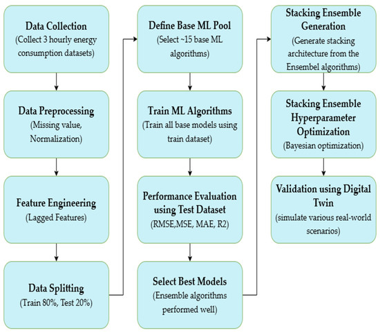
Figure 2.
Overview of the SEF-SDT approach.
2.5. Identification of the Machine Learning Pool and Stacking Layers
The base learners (Layer 1) constitute the initial layer of the stacking model. They are employed to capture various patterns within the energy consumption data and generate initial predictions. At this layer, a heterogeneous algorithm pool was created from various ML algorithms. This diverse structure allows the stacking model to learn a wide range of data patterns by utilizing each algorithm’s unique strengths. This approach helps optimize the bias-variance trade-off and enhances the model’s generalizability [29]. The selected base learners, explained in the following sections, include 15 diverse algorithms (e.g., linear regressors, tree-based ensembles, support vector machines, neural networks).
2.5.1. Linear and Regularized Regression Models
This group of models aims to find a linear function of the form best fits the observed data. To prevent overfitting, regularization terms are added to the cost function to decrease model complexity. Poisson and Tweedie regressors are generalized linear models that generate this linear relationship with a function that handles different distributions of the target variable. In this work, the models selected in this category include ElasticNet, Lasso, LassoLars, the Passive Aggressive Regressor, the Poisson Regressor, the Tweedie Regressor, and the RANSAC (RANdom SAmple Consensus) Regressor [29,30].
2.5.2. Single-Tree Models
These models recursively divide the dataset based on feature values. They then provide the average of samples in each leaf node as the prediction, with the aim of minimizing a loss function like Mean Squared Error (MSE) within each node. This loss is expressed as . Here, represents a leaf node, and is the average target value of the samples in that node. The algorithm used from this model group in the study is Decision Tree Regressor [29,30].
2.5.3. Support Vector Machines (SVM)
SVM algorithms are effective in both linear and non-linear regression problems. They handle complex patterns by mapping data to high-dimensional spaces. The goal is to find a hyperplane () that contains as many data points as possible within a ϵ-insensitive tube (also known as an error tolerance zone). Kernel functions (Polynomial, RBF) help to model non-linear relationships by mapping low-dimensional data into a high-dimensional feature space. In this work, SVR models having poly and radial basis function (RBF) kernels were selected in the base learner pool [29,30].
2.5.4. K-Nearest Neighbors Regressor (KNR)
KNR models are non-parametric algorithms that capture local patterns using similarity measures. They derive a data point’s prediction from the characteristics of its nearest neighbors. The prediction for a new query point, , is made by averaging the average of the target values () of its nearest neighbors from the training set, as shown in Equation (5).
Here, is the set of K-nearest training points to . Proximity is generally determined by a metric such as Euclidean distance [29,30]. As a non-parametric model, KNR is a particularly valuable local modeling algorithm, adding diversity to the base learner pool.
2.5.5. Artificial Neural Network (ANN)
Multi-layer perceptron-based models are capable of learning complex, non-linear relationships. An ANN consists of an input layer, one or more hidden layers, and an output layer. Each neuron (node) produces an output by applying an activation function to the weighted sum of the inputs (). The backpropagation algorithm updates the model’s weights and biases by using the error propagated through the network. This error is typically generated by a loss function like MSE. Gradient descent (or its variations) is used to minimize the loss function. From the ANN algorithm group, the MLP was selected for the base learner pool [29,30].
2.5.6. Ensemble Learning via Boosting
Boosting algorithms generally create a powerful model by combining weak learners. Algorithms in this group, such as Gradient Boosting Machine (GBM) and Extreme Gradient Boosting (XGBoost) regressors, are trained to correct the errors of the previous model iteratively. This method updates the model by adding a new learner that minimizes a loss function, which can be expressed as . In this expression denotes the new weak learner. However, Adaptive Boosting (AdaBoost) uses a different method by assigning higher weights to samples that were predicted incorrectly. In this study, the GBM, XGBoost, and AdaBoost models were used to represent these approaches for the base learner pool [29,30].
2.5.7. Ensemble Learning via Bagging
Bagging methods reduce overfitting and improve generalizability by training decision trees in parallel. The main principle of bagging is to train independent base learners on bootstrap samples of the training data and combine their predictions. For regression problems, the final prediction is obtained by averaging the outputs of these independent learners, as shown in Equation (6).
This approach reduces the variance of high-variance models (e.g., decision trees), thus increasing model stability and reducing overfitting. In this study, the Random Forest Regressor (RFR) was selected to represent this approach [31].
For the second layer of the stacked ensemble, the Extra Trees Regressor (ETR), a bagging ensemble model, was chosen as the meta-learner. This selection was made because ETR effectively generalizes unseen data and efficiently reduces prediction variance. These advantages come from its extreme randomness, achieved by using the entire dataset and randomly selecting split points during its training process.
2.5.8. Meta-Learner Selection for Stacking
The base learner pool was designed with diversity in mind. Diversity allows each model in the pool to have unique bias-variance trade-off characteristics. For example, while linear models typically have high bias and low variance, single decision trees show high variance and low bias. On the other hand, while boosting algorithms focus on reducing bias, bagging algorithms aim to decrease variance. The strength of the stacking ensemble in this context is its ability to minimize the errors produced by diverse base algorithms [32]. Mathematically, the variance of an ensemble’s prediction is related to the average variance of individual ML models and their corresponding correlations, as expressed in Equation (7).
Here, is the number of models, is the average variance of individual models, and is the average correlation between them. Stacking is effective due to low correlations among base models, which considerably reduces the overall variance. Using the predictions of base learners as “meta-features”, the meta-learner yields a more robust and generalizable final prediction. In general, stacking uses only Level 1 predictions as input. In the proposed stacking scheme, the meta-learner’s input was enhanced with both base model predictions and derived lagged features. In this way, the proposed stacking with augmented features captures (i) relationships learned by the base models and (ii) temporal patterns from lagged features, leading to enhanced final predictions.
As previously noted, the ETR was chosen as the meta-learner (Level 2) for its advanced variance reduction ability. Its “extra randomness” (using the entire dataset and random split points) generates trees with less correlation. This is ideal for a meta-learner, enabling effective combination of base model (Level 1) predictions with uncorrelated errors. Furthermore, ETR can identify complex non-linear relationships. Since ETR has natural resistance to overfitting, it is well-suited for learning the detailed patterns within the augmented meta-features [33].
2.6. Model Performance Evaluation Criteria: Metric Selection
An appropriate selection of performance metrics is important for evaluating the success of forecasting models. RMSE was chosen as the primary metric for experimental comparisons. To provide a comprehensive evaluation of model performances, Mean Absolute Error (MAE), Coefficient of Determination (R2), and Mean Absolute Percentage Error (MAPE) were also used as supportive metrics. These metrics are expressed mathematically in Equations (8)–(11) as follows:
- Root Mean Squared Error (RMSE):
- Mean Absolute Error (MAE):
- Coefficient of Determination (:
- Mean Absolute Percentage Error (:
RMSE measures how large the prediction error is, and its unit matches the target variable’s unit (e.g., KWh). The formula, given in Equation (8), calculates the square root of the average of squared differences between actual and predicted values. Here, N represents the number of data points, is the actual value, and is the predicted value. This makes the error easy to understand in a real-world context [9,29]. A lower RMSE indicates that more accurate predictions are made by models. Because errors are squared, RMSE is strongly affected by large mistakes. This offers a major advantage in energy forecasting, as significant errors during peak demand are highly costly and can impact grid stability [9,29]. Furthermore, since RMSE is widely used in energy research literature, SEF-SDT model outcomes can be compared with other studies. For all these reasons, RMSE was chosen as the main evaluation metric. The other metrics, i.e., R2, MAE, and MAPE, are evaluated as follows. R2, or the coefficient of determination, shows how well the independent variables explain the variation in the dependent variable. The formula, given in Equation (10), compares the model’s error to the variance of the actual data. The values closer to 1 indicate a stronger fit and better explanatory power. A value of 0 indicates that the model is no better than simply predicting the mean of the data, while a negative value suggests that the model performs even worse than that, indicating a very poor fit. MAE measures the average magnitude of prediction errors in the dependent variable. This metric is less sensitive to large outliers compared to RMSE because it takes the absolute value of the errors instead of squaring them. Here, N represents the number of data points, is the actual value, and is the predicted value. Lower MAE values indicate higher prediction accuracy. Lastly, MAPE provides the mean absolute percentage error. It is particularly useful for comparing accuracy across different scales due to its normalization. This metric is defined by Equation (11), where N is the number of data points, is the actual value, and is the predicted value. It is important to note that MAPE can be unstable or undefined when actual values are close to zero. Lower percentages denote better predictive performance.
2.7. Data Splitting and Training of Machine Learning Algorithms
For proper model evaluation and generalization, the dataset was initially divided into 80% training and 20% testing sets to prevent data leakage. This method was applied to both Level 1 (base learners) and Level 2 (meta-learner) learners. The base algorithms of SEF-SDT were trained using the training data. The base algorithms were trained using the training data, and in this stacking approach, 5-fold cross-validation was used to produce their out-of-fold predictions. These predictions and lagged features are then combined to train the meta-learner. The testing set was consequently used to evaluate the entire model’s performance without bias. The selection of base algorithm subset and the meta-learner for the final model were chosen by minimizing RMSE, while also considering complementary metrics (i.e., MAE, R2, and MAPE). This method of selection is explained in detail in the following section.
2.8. Model Selection with Random Search Optimization for Stacking Generation
Having obtained the experimental results, the Level 1 (base learner) and Level 2 (meta-learner) models for the stacking architecture must be selected to create the SEF-SDT model’s ensemble. At this stage, the selection of the base learners from the algorithm pool was performed using the Random Search algorithm. This selection mainly aimed to find the most accurate algorithms on each of the three datasets by minimizing the RMSE value. From many combinations generated through Random Search, AdaBoost Regressor and Gradient Boosting Regressor were ultimately chosen as the L1 layer (base learners) for the stacking ensemble. Despite having many options for the Layer 2 (L2) meta-learner, Extra Trees Regressor was rationally selected based on the motivations provided in Section 2.5.8.
In model selection, various search algorithm options are available, including systematic approaches like Grid Search, adaptive methods like evolutionary algorithms, and strategies such as Random Search, which can efficiently explore search spaces. Random Search was chosen to determine the final algorithm subset for this stacking architecture. Its strong exploration capabilities in large and high-dimensional search spaces made it an appropriate choice, especially when compared to systematic methods like Grid Search [34]. Grid Search’s computational cost grows exponentially with the search space. This makes evaluating combinations of 15 algorithms for stacking computationally expensive. In contrast, Random Search can efficiently identify effective algorithms by sampling randomly at a lower computational cost [34]. Evolutionary methods, like genetic algorithms, can also explore the search space adaptively. However, they are more complex to implement, and their search process is computationally intensive [34]. On the other hand, Random Search’s simplicity and computational efficiency were key factors in its selection for this stage. As stated previously, the goal of Random Search was to discover the optimal ML algorithms for the L1 layer of the stacking ensemble. This process aimed to minimize the designated metric, RMSE. This approach produces a high-performing stacking model. Additionally, the hyperparameters of this final stacking model are then explored to enhance its performance through a Bayesian Optimization step, which is detailed in the following section.
2.9. Bayes Hyperparameter Optimization of the Final Stacking Ensemble Model
Having obtained the subset of algorithms that constitutes the final stacking model, its further improvement and exploration through parameter tuning is a standard practice in ML literature. In this work, therefore, we tuned the hyperparameters of the final stacking model, which includes both its L1 layer algorithms (AdaBoost Regressor and Gradient Boosting Regressor) and its L2 layer algorithm (Extra Trees Regressor). This tuning was performed using a Bayesian Optimization step. Bayesian Optimization (BO) is a model-based framework that provides an efficient exploration strategy for complex, computationally expensive objective functions, like evaluating an entire ensemble model via cross-validation [35]. Unlike methods that sample in a non-adaptive manner, such as Grid Search or Random Search, BO intelligently learns from past trials. It constructs a probabilistic approximate model (typically a Gaussian Process) to predict the performance of untested hyperparameter combinations. At each iteration, an acquisition function (like Expected Improvement) selects the next most suitable trial point. The function handles this by logically balancing two objectives: (i) exploring new, unknown regions of the hyperparameter space, and (ii) exploiting the high-performing areas that are already known [35]. This process continues iteratively until the optimal hyperparameters that minimize the objective function are identified.
The obtained results of the optimized Stacking-Final model, as presented in Section 3.1, are compared with those of the best-performing baseline model, Gradient Boosting Regressor. The significant improvement of the proposed model is confirmed using statistical analysis, including the Wilcoxon signed-rank test [36].
In this work, the main objective was to minimize the RMSE value by optimizing the performance of the stacking model across all three datasets. This involved simultaneously optimizing the hyperparameters of both the L1 learners and the L2 meta-learner of the entire stacking ensemble. This iterative process systematically increased the generalizability and prediction accuracy of the developed stacking model across datasets. While the BO tuning step decreased RMSE for the Diyarbakır (2.98% reduction) and Odemis (4.79% reduction) datasets, it showed no significant change for the Istanbul dataset. The quantitative details are explained in the Results and Discussion section.
2.10. Simulation-Based Digital Twin with Real-World Test Scenarios
The sustainable operation of modern energy systems relies heavily on the accuracy of short-term energy consumption forecasting models. However, if real-time sensor data is limited or unavailable, it is almost impossible to fully check a model’s true performance under real-world conditions, as is the case in this study. To address this challenge and test the developed stacking model, we implemented simulation-based scenarios based on Digital Twins (DTs). This approach enabled the generation of various test conditions and validated the model’s practical applicability in a controlled simulation environment, without real-time streaming data available.
The creation of Digital Twin simulations through software has great potential for the design, operation, and optimization of complex systems across various industries [37]. In this manner, such software implementations are important as they provide the necessary modeling, simulation, visualization, and analysis capabilities for Digital Twin development [37]. From this perspective, a Digital Twin (DT) can be defined as a dynamic virtual representation of a physical entity or process, with software implementation being one of its core components [37]. Simulation, a key part of DTs, has been successfully applied in critical areas such as load forecasting and energy efficiency optimization in energy systems [38]. The simulation-based flexibility of the proposed SDT structure proved valuable for scenario-driven forecast validation, particularly when real data streams were irregular or limited. This provided a basic validation step for the model’s potential future integration into DT-based energy management systems.
Before presenting the details of the simulated scenarios, it is important to understand how these scenarios were generated and their role in the model evaluation process. In this context, it should be noted that the four simulation scenarios were generated by applying the described modifications to the pre-split test dataset, ensuring the model had not previously seen these specific conditions during its training. For each scenario, the model’s performance on the original test set was then quantitatively compared with its performance on the modified test data. Hence, the four scenarios designed as real-world conditions are (i) Behavioral Change, (ii) Data Quality and Reliability, (iii) Device Failure, and (iv) Energy Efficiency Upgrade, and they are briefly explained as follows:
- (i)
- Behavioral Change Test Scenario: This scenario evaluates the model’s adaptation capability by simulating the long-term and short-term impacts of human behavior on energy consumption patterns.
- Structural Change (Evenings 18:00–23:45): This represents a long-term change in user behavior (e.g., an increase in time spent at home in the evenings). In the simulation, energy usage during these evening hours was increased by 20% across the test dataset. This sub-scenario aims to test the model’s ability to adapt to permanent changes in routine over time.
- Sudden Change (Sudden Peaks on all Weekends): This simulates a temporary and sudden increase in usage (e.g., special events, hosting guests, or prolonged periods at home). In the simulation, a sudden 50% spike in energy consumption was injected only on weekends. This sub-scenario aims to evaluate the model’s ability to detect and manage unexpected, short-term, high-amplitude consumption anomalies.
- (ii)
- Data Quality and Reliability Test Scenario: This scenario simulates real-world data issues to evaluate the model’s robustness and its ability to minimize performance decrease when inputs are unreliable. The simulated data issues include (a) Missing Timestamps, which are gaps in time-series data simulating interruptions in sensor readings; (b) Outlier or Unrealistic Values, which are measurement errors containing abnormally high or low values (e.g., 100 times the normal consumption); (c) Sensor Noise, which consists of random fluctuations added to the data caused by faulty measurement equipment; (d) Timestamp Shift, which represents misaligned time labels (e.g., shifts of a few minutes or hours); and (e) Combined Corruption, which is the application of all the above data quality issues together. The objective is to test the forecast model’s elasticity and error tolerance against common real-world data challenges.
- (iii)
- Device Failure Test Scenario: This scenario simulates a localized, hardware-level anomaly, such as a device (e.g., an air conditioner) malfunctioning and consuming an abnormally high amount of power. For instance, energy consumption was artificially increased by 20% during a specific time window. The objective is to test whether the model can detect or adapt to specific, localized, and non-persistent anomalies caused by faulty equipment.
- (iv)
- Energy Efficiency Upgrade Test Scenario: This scenario models long-term, gradual improvements in building energy efficiency. Examples include the installation of LED lighting, adding insulation, or upgrading to energy-efficient appliances. In the simulation, a gradual decrease of 15% in energy usage was applied after a specific time index. The objective is to observe how well the model adapts to gradual, long-term shifts in consumption baselines.
This evaluation strategy systematically measures the model’s robustness and proceeds as follows. First, we established a baseline RMSE on the clean, pre-split test set for each of the three cities. Next, as previously explained, we generated the four simulation scenarios by applying the described modifications to this test dataset. We then re-evaluated the model on each of the newly modified datasets to obtain the scenario-specific performance. The results were analyzed by comparing the initial baseline scores against the scores from the modified data, and the corresponding performance graphs were plotted. The detailed findings of this extensive evaluation are presented in Section 3.1.
The complete process of the proposed SEF-SDT methodology is detailed in pseudocode format as shown in Appendix A.
3. Results and Discussion
In this section, we present the detailed experimental results obtained from this study and discuss the corresponding insights. This includes the development and detailed evaluation of the stacked ensemble models, their optimization processes, and their integration for scenario-based real-world testing within a simulation-based Digital Twin environment.
3.1. Evaluation of ML Algorithms in Predictive Performance
As detailed in the Methodology section, we obtained three household energy consumption datasets: Diyarbakir, Istanbul, and Odemis. We preprocessed these datasets, including min-max normalization for feature scaling and outlier detection with mean imputation, ensuring data quality and model robustness.
In the feature engineering phase, we generated temporal features: lag_1 (past 1 h), lag_24 (past 1 day), and lag_168 (past 1 week) to capture consumption dynamics over time.
The rationale for the selection of these specific features was established through an autocorrelation analysis. This analysis revealed strong positive correlations for all three lags across the three cities. The coefficients for lag_1 were 0.86 for Istanbul, 0.67 for Diyarbakir, and 0.62 for Odemis. Similarly, lag_24 and lag_168 also demonstrated statistically significant correlations across all datasets. These statistically significant findings, confirming the existence of strong temporal dependencies, are visually presented in Figure 3.
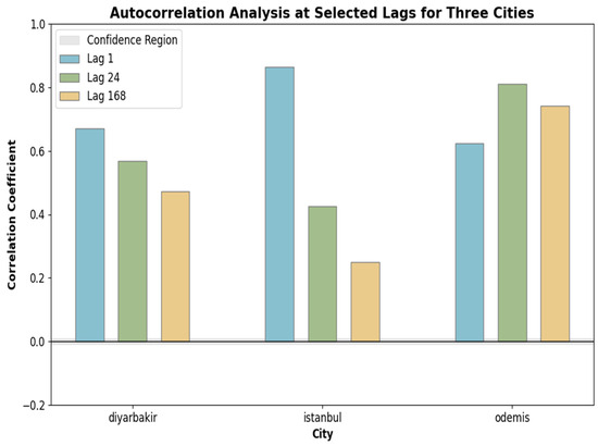
Figure 3.
Autocorrelation coefficients at selected lags (1, 24, and 168 h) in Istanbul, Diyarbakir, and Odemis.
To further investigate the relationships between the engineered features and the target variable, a correlation heatmap was generated. Figure 4 presents a correlation heatmap visualizing the relationship between these engineered features and the target variable (current energy consumption). The heatmap clearly indicated a strong positive correlation for lag_1 (0.847), confirming the high sequential dependency of energy consumption data. Even having weaker negative correlations, lag_24 and lag_168 were kept for their role in capturing daily and weekly patterns, providing valuable context for advanced models.
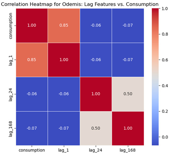
Figure 4.
Correlation heatmap of lagged features with energy consumption feature.
For experimental evaluation, 15 diverse Machine Learning algorithms formed the baseline learner pool. Datasets were split 80% for training and 20% for testing (also used for data simulations of the mentioned scenarios) without shuffling, to preserve temporal order crucial for time-series forecasting. RMSE served as the primary performance metric, supplemented by R2, MAE, and MAPE for a detailed assessment. We evaluated all 15 baseline algorithms across the Diyarbakır, Istanbul, and Odemis datasets. This initial evaluation helped to observe the general performance of the models and to identify promising candidates for the ensemble. Table 2 presents a comprehensive overview of the performance of all baseline algorithms, and the standard, enhanced, and Bayesian Optimized stacking models in terms of RMSE, R2, MAE, and MAPE.
Table 2.
A comprehensive overview of the performance of all baseline algorithms, and our standard, enhanced, and Bayesian Optimized stacking models.
The initial evaluation, summarized in Table 2, shows several important findings about the prediction accuracy of the baseline and stacked ensemble models for energy consumption forecasting across the three cities.
All stacking models use an L1 layer made of AdaBoost and Gradient Boosting Regressor, with Extra Trees Regressor as the L2 (meta) learner.
Initially, across all cities, ensemble algorithms like Gradient Boosting Regressor, RandomForest, and XGBoost generally performed better than single ML models. For instance, Gradient Boosting Regressor performed well, with RMSEs of 0.1348 in Diyarbakır, 0.0460 in Istanbul, and 0.0792 in Odemis. Similarly, RandomForest and XGBoost also produced good RMSE values with generally higher R2 scores. In this manner, they essentially fit the data better than simpler models like Lasso or ElasticNet (showing negative R2 values for some datasets). Algorithms like Passive Aggressive Regressor performed poorly across all metrics, clearly showing they were not appropriate for this prediction task.
The standard stacking model (which uses only the L1 algorithm predictions as features) delivered clear improvements compared to the baseline algorithms. In Diyarbakır, it decreased RMSE by 5.42% (from 0.1348 to 0.1275) compared to the best baseline, Gradient Boosting Regressor. For Istanbul, while its RMSE is the same as RandomForest (0.0453), it improved MAE by 31.34% (from 0.0284 to 0.0195). Additionally, compared to Gradient Boosting’s MAPE of 96.52, Standard Stacking greatly decreased Istanbul’s MAPE to 10.96. In Odemis, it achieved a 6.82% decrease in RMSE (from 0.0792 to 0.0738) and a 48.51% drop in MAPE (from 49.87 to 25.68) over Gradient Boosting Regressor.
The enhanced stacking model (which includes lagged features in addition to L1 algorithm predictions) further improved prediction accuracy, always providing the lowest RMSE values across all three cities. For Diyarbakır, it decreased RMSE by 17.80% (from 0.1348 to 0.1108) and a 19.91% drop in MAPE (from 51.39 to 41.16) compared to the best single model. For Istanbul, the enhanced stacking showed a 5.87% drop in RMSE (from 0.0460 to 0.0433) and a 6.15% decrease in MAE (from 0.0195 to 0.0183, compared to standard stacking), with the best R2 of 0.7498. In Odemis, the algorithm achieved a 7.70% decrease in RMSE (from 0.0792 to 0.0731) and a remarkable 53.82% drop in MAPE (from 49.87 to 23.03) against the best single model.
Experimentally, the enhanced stacked ensemble proved to be the most accurate model across all tested datasets in terms of the three metrics. These results support the idea that mixing strong base learners with feature engineering considerably improves energy consumption prediction accuracy. While some single models performed satisfactorily, combining them through stacking variations consistently produced enhanced results with percentage improvements across all metrics in three cities. While Table 2 summarizes the overall performance metrics, we present a visual analysis of the model’s performance (true vs. predicted) for three cities after obtaining the optimized final stacking model.
3.2. Hyperparameter Tuning of Stacking Ensemble with Bayesian Optimization
Generally, even the best ML models can benefit from optimization to improve performance. Therefore, the hyperparameters of the enhanced stacked model’s constituents (AdaBoost Regressor, Gradient Boosting Regressor, and Extra Trees Regressor) discussed in the previous section were carefully optimized using Bayesian Optimization for each city dataset. This process aims to minimize RMSE by exploring the parameter space of algorithms. Table 3 presents the optimal hyperparameters found for Diyarbakır, Istanbul, and Odemis datasets, respectively.
Table 3.
Optimal hyperparameters for enhanced stacked ensemble model (Bayesian Optimization).
Bayesian Optimization considerably refined the enhanced stacked ensemble model, resulting in performance improvements. Comparing these optimized results to the non-optimized enhanced stacking model (also presented in Table 2), the performance improvements are as follows:
- (i)
- Diyarbakır: RMSE improved by 3.88% (0.1108 to 0.1065), MAE by 5.35% (0.0795 to 0.0755), R2 increased by 9.5% (0.4445 to 0.4868), and MAPE decreased by 7.02% (41.16 to 38.28).
- (ii)
- Istanbul: MAE decreased by 2.19% (0.0183 to 0.0179) and MAPE by 4.43% (10.82 to 10.34). While RMSE increased minimally (0.0433 to 0.0436), R2 remained high at 0.7471, indicating that the model was already robust.
- (iii)
- Odemis: RMSE improved by 4.79% (0.0731 to 0.0696), MAE by 6.28% (0.0478 to 0.0448), R2 increased by 3.92% (0.7020 to 0.7295), and MAPE decreased by 6.86% (23.03 to 21.45).
In summary, Bayesian Optimization effectively tuned parameters of the enhanced stacked ensemble model, resulting in notable accuracy and reliability improvements across all three datasets.
We present experimental results for stacking and enhanced stacking versions compared to baseline algorithms numerically using Table 2. Following the optimization of the enhanced stacking model, we aim to present the model’s efficiency in hourly energy consumption prediction for Istanbul, Diyarbakır, and Odemis. To this end, we plotted Figure 5, Figure 6 and Figure 7 to visually demonstrate the predictive capacity of the optimized stacking model.
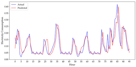
Figure 5.
Hourly performance of optimized stacking model: actual vs. predicted energy values for Istanbul.
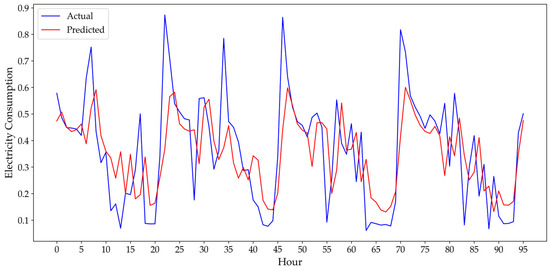
Figure 6.
Hourly performance of optimized stacking model: actual vs. predicted energy values for Diyarbakir.
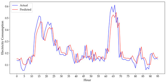
Figure 7.
Hourly performance of optimized stacking model: actual vs. predicted energy values for Odemis.
As can be seen from Figure 5, Figure 6 and Figure 7, the final optimized stacking model demonstrates strong performance in adapting to the variations of hourly consumption patterns in three cities. More precisely, for Istanbul (Figure 5), the predicted hourly energy consumption values closely track the actual consumption, successfully adapting to both the regular, cyclical fluctuations and sudden changes. This visual performance is consistent with the positive numerical results obtained after Bayesian Optimization, which led to a notable decrease in MAE and MAPE. Similarly, the plot for Diyarbakır (Figure 6) visually confirms the model’s high accuracy, reflecting the significant improvements in RMSE (3.88%) and MAE (5.35%) after optimization. Lastly, the plot for Odemiş (Figure 7) demonstrates how effectively the model captures the consumption patterns of the city, which is numerically supported by a 4.79% improvement in RMSE and a 6.28% improvement in MAE. These plots visually illustrate the final model’s efficiency in terms of actual vs. predicted consumption.
To statistically validate the improvements observed in predicted energy consumption across the three cities, a Wilcoxon signed-rank test was conducted comparing the proposed Stacking-Final ensemble model against the best-performing baseline, Gradient Boosting Regressor.
The Wilcoxon signed-rank statistical analysis of the proposed Stacking-Final ensemble model in comparison to the Gradient Boosting Regressor is shown in Table 4. The Wilcoxon signed-rank test determines whether the results of the two models exhibit a statistically significant difference. A (p-value) < 0.05 indicates significant superiority [36]. The positive and negative rank sums indicate the total ranks of observations where StackingFinal outperforms or underperforms Gradient Boosting Regressor, respectively. The reported Sum of Signed Ranks (W) corresponds to the smaller of the positive and negative rank sums, as is standard in the Wilcoxon signed-rank test. The hypothesis testing is formulated as follows:
Null hypothesis (H0).
µ_StackingFinal = µ_GradientBoostingRegressor.
Alternate hypothesis (H1).
µ_StackingFinal ≠ µ_GradientBoostingRegressor.
Table 4.
Wilcoxon signed-rank test results comparing the proposed Stacking-Final model with Gradient Boosting Regressor across three cities.
Table 4.
Wilcoxon signed-rank test results comparing the proposed Stacking-Final model with Gradient Boosting Regressor across three cities.
| City | Sum of Signed Ranks (W) | Positive Rank Sum | Negative Rank Sum | p Value (Two-Tailed) | Exact/Estimate | Significant (α = 0.05) |
|---|---|---|---|---|---|---|
| Diyarbakır | 3 | 195 | 3 | 0.00121 | Exact | Yes |
| Istanbul | 10 | 280 | 10 | 0.00305 | Exact | Yes |
| Odemis | 8 | 484 | 8 | 0.00089 | Exact | Yes |
As shown in Table 4, the p-values are less than 0.05 for all three cities (Diyarbakır, Istanbul, Odemis), demonstrating that Stacking-Final achieves lower RMSE values compared to Gradient Boosting Regressor. This confirms the superiority of the Stacking-Final ensemble model and indicates the statistical significance of the improvement. Therefore, the alternate hypothesis H1 is accepted.
Having statistically validated the model with the Wilcoxon test, we next focus on the primary objective of this study: developing and optimizing a high-performing energy consumption forecasting model across three cities. To assess the optimized model’s robustness and generalization capabilities in diverse real-world contexts, the subsequent section details its performance through a comprehensive simulation-based Digital Twin (SDT) framework.
3.3. Model Performance: Scenario-Based Testing with Simulated Digital Twin
To formally define the data transformations used for scenario-based testing, each modification was systematically applied to the original test dataset to create a new, modified test set. The model’s performance was then evaluated on these modified datasets and compared against its baseline performance on the original, unmodified test data. The specific transformations for each scenario are defined as follows:
- (i)
- User Behavioral Changes Scenario: To simulate changes in user consumption habits, two distinct transformations were applied. The Structural Change involved a persistent modification of consumption values during the evening hours (18:00–23:45), scaling them by a constant multiplicative factor of 1.20. The Sudden Change modeled unexpected anomalies by introducing temporary spikes, where consumption values on randomly selected weekend periods were scaled by a multiplicative factor of 1.50.
- (ii)
- Data Quality and Reliability Scenario: This scenario assessed the model’s resilience to common data issues by synthetically corrupting the test dataset. Missing data was simulated by randomly masking data points. Outliers were introduced by replacing a subset of data points with statistically significant deviations from their expected values. Sensor noise was generated by adding random Gaussian noise to consumption values. Timestamp drift was simulated by synthetically shifting data points by a small offset. The Combined Corruption scenario involved simultaneously applying all four of these individual transformations to the same test dataset.
- (iii)
- Appliance Malfunction Scenario: A localized, hardware-induced anomaly was simulated by selecting a time window and scaling all consumption values within that window by a multiplicative factor of 1.20, representing an appliance drawing 20% more power.
- (iv)
- Energy Efficiency Upgrade Scenario: This scenario evaluated the model’s ability to adapt to gradual, long-term changes by simulating a continuous, proportional reduction in energy usage. Starting from a specified time index, all subsequent consumption values were scaled by a multiplicative factor of 0.85, simulating a gradual 15% reduction.
The following sections present a detailed analysis of the final model’s predictive performance and robustness under each of the defined scenario-based data transformations.
3.3.1. User Behavioral Changes Scenario
This scenario investigated the model’s adaptability to variations in human energy consumption behavior by simulating two distinct types of changes. The Structural Change (Evening Hours 18:00–23:45) scheme involved a persistent 20% increase in energy consumption during evening hours, evaluating the model’s ability to adapt to these usage routines. Conversely, the Sudden Change (Sudden Spikes on Weekends) test simulated temporary 50% spikes in weekend energy consumption, assessing the model’s capacity to manage unexpected anomalies. The RMSE performance metrics for the final model under these two scenarios are presented in Table 5. This includes the RMSE from the model’s standard test data prediction mode (normal operation) for comparison.
Table 5.
Final model performance (RMSE) under behavioral tests.
The results show varying degrees of model robustness. For the Structural Change, the model demonstrated strong adaptability in Diyarbakır with a minimal RMSE increase (0.1065 to 0.1082). This suggests effective handling of gradual shifts. While Istanbul and Odemis showed some sensitivity with noticeable RMSE increases (0.0436 to 0.0519 and 0.0696 to 0.0842, respectively), the Sudden Spikes on Weekends generally presented a greater challenge across all cities. Particularly, Odemis experienced the most considerable impact, with RMSE significantly increasing to 0.2469. This highlights the difficulty in predicting extreme, concentrated anomalies, suggesting the possible need to retrain models with new data.
Overall, the model reveals good resilience to the Structural Changes, adapting well to new routines. However, the Sudden Spikes on Weekends lead to more obvious error increases. These findings emphasize the need for dynamic anomaly detection and potentially adaptive retraining to maintain optimal performance during extreme human-driven consumption changes.
Following the optimization of the enhanced stacking model, we visually demonstrate the model’s predictive performance under these two scenarios. The figures detailing the model’s performance under the Structural Change scenario are presented below:
Figure 8, Figure 9 and Figure 10 visually demonstrate the model’s predictive performance under the Structural Change scenario for Diyarbakır, Istanbul, and Odemis. These plots reveal the model’s overall strong performance in adapting to new routines. More specifically, for Diyarbakır (Figure 8), the predicted values closely follow the new, higher consumption patterns, which align with the minimal RMSE increase seen in Table 5. Similarly, Figure 9 for Istanbul and Figure 10 for Odemis show that the model generally captures the shifted consumption patterns well, despite the moderate increases in RMSE. These visualizations confirm the model’s resilience to gradual, persistent changes in user behavior, effectively adapting its predictions to the new consumption routines. For the ‘Sudden Spikes on Weekends’ scenario, the figures detailing the model’s performance are presented below:
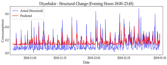
Figure 8.
Predictive performance of the model under structural change scenario in Diyarbakır: actual vs. predicted energy values.
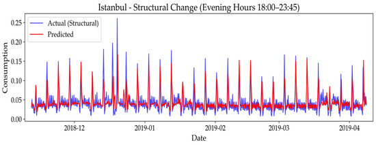
Figure 9.
Predictive performance of the model under structural change scenario in Istanbul: actual vs. predicted energy values.
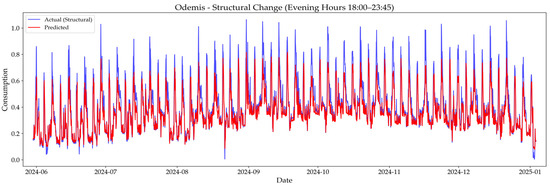
Figure 10.
Predictive performance of the model under structural change scenario in Odemis: actual vs. predicted energy values.
Figure 11, Figure 12 and Figure 13 visually confirm the increased challenge presented by these temporary anomalies. The plots for Diyarbakır (Figure 11), Istanbul (Figure 12), and Odemis (Figure 13) all show larger discrepancies between actual and predicted values during the sudden spikes on weekends. This is particularly evident in Figure 13 for Odemis, where the model’s prediction line fails to capture the extreme peak, directly correlating with the significant RMSE increase to 0.2469 noted in Table 5. These figures collectively underscore the difficulty in accurately forecasting extreme and concentrated anomalies, highlighting the need for dynamic anomaly detection and retraining strategies to maintain optimal performance in the face of such abrupt behavioral changes.

Figure 11.
Predictive performance of the model under sudden spikes on weekend scenario in Diyarbakır: actual vs. predicted energy values.
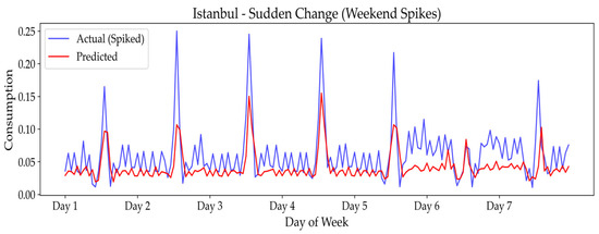
Figure 12.
Predictive performance of the model under sudden spikes on weekend scenario in Istanbul: actual vs. predicted energy values.
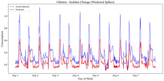
Figure 13.
Predictive performance of the model under sudden spikes on weekend scenario in Odemis: actual vs. predicted energy values.
3.3.2. Data Quality and Reliability Scenario
This scenario assessed the model’s robustness against common real-world data reliability problems, simulating the following data issues: Missing Timestamps, Outliers, Sensor Noise, Timestamp Drift, and an overall combined corruption scenario. The primary purpose was to stress-test the model’s resilience to faulty data, a critical challenge for reliable Digital Twin integrated operations. Table 6 presents the RMSE performance metrics under these scenarios.
Table 6.
Final model performance (RMSE) under data quality tests.
The final model generally showed strong resilience to these data quality issues. For individual data corruptions like Missing Data or Timestamp Drift, the RMSE showed minimal to no impact across all cities, often matching Normal Operation values (e.g., Diyarbakır 0.1041). Outliers and Sensor Noise introduced only slight RMSE increases, maintaining high model accuracy. Even under Combined Corruption, where all issues were simultaneously present, the RMSE increases remained relatively limited and manageable across Diyarbakır (0.1112), Istanbul (0.0500), and Odemis (0.0745). This demonstrated the model’s robustness against multilayered real-world data challenges. This strong performance against common data quality and reliability issues is critical for Digital Twin simulations, ensuring consistent and reliable insights despite imperfect real-world data inputs.
While this scenario group comprises four sub-scenario types across three cities, potentially requiring 12 figures, the RMSE values for each individual data issue did not exhibit substantial differences. Consequently, to avoid redundancy, Figure 14, Figure 15 and Figure 16 are presented below to visually demonstrate the model’s predictive performance under the most challenging, combined corruption scenario.
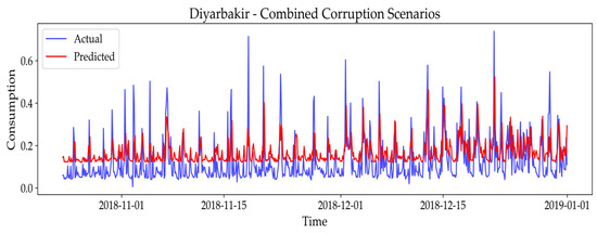
Figure 14.
Predictive performance of the final model under combined corruption scenario in Diyarbakır: actual vs. predicted energy values.

Figure 15.
Predictive performance of the final model under combined corruption scenario in Istanbul: actual vs. predicted energy values.
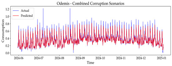
Figure 16.
Predictive performance of the final model under combined corruption scenario in Odemis: actual vs. predicted energy values.
As evident from both the RMSE-based analysis and Figure 14, Figure 15 and Figure 16, the final model demonstrates high robustness against the data issues in all city datasets. The plots for Diyarbakır (Figure 14), Istanbul (Figure 15), and Odemis (Figure 16) visually confirm that the predicted values remain remarkably close to the corrupted actual data, effectively maintaining predictive accuracy despite the presence of missing data, outliers, sensor noise, and timestamp drift. This strong capability to handle a multilayered data integrity problem is critical for ensuring reliable insights in Digital Twin simulations.
3.3.3. Appliance Malfunction Scenario
This scenario simulates a hardware-level anomaly: a single appliance consuming 20% more power within a selected time window. The test aimed to evaluate the model’s adaptability to such localized, equipment-induced anomalies. Table 7 presents the RMSE performance metrics for the optimized enhanced stacked model under this scenario.
Table 7.
Final model performance (RMSE) under appliance malfunction scenario.
The ‘Appliance Malfunction Scenario’ impacted the model’s predictive accuracy differently across cities. Istanbul demonstrated remarkable stability with a minimal RMSE increase (0.0436 to 0.0443), showing high robustness to equipment failures. Diyarbakır also adapted well, displaying only a small RMSE rise (0.1065 to 0.1130). On the other hand, Odemis experienced a more significant impact, with RMSE increasing notably from 0.0696 to 0.1095.
While Table 7 presents the numerical analysis of the final model’s response to equipment malfunction, Figure 17, Figure 18 and Figure 19 visually demonstrate the model’s predictive performance under the same scenario for Diyarbakır, Istanbul, and Odemis.
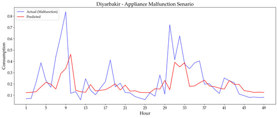
Figure 17.
Predictive performance of the final model under appliance malfunction scenario in Diyarbakır: actual vs. predicted energy values.
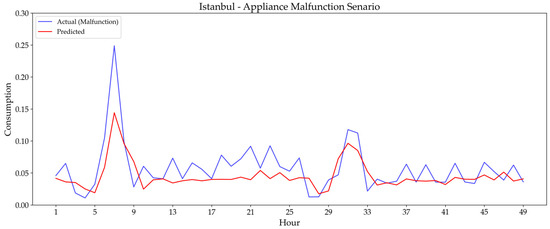
Figure 18.
Predictive performance of the final model under appliance malfunction scenario in Istanbul: actual vs. predicted energy values.
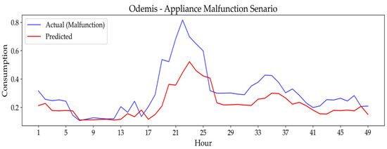
Figure 19.
Predictive performance of the final model under appliance malfunction scenario in Odemis: actual vs. predicted energy values.
The plots show how the model’s predictive accuracy is impacted differently across cities. For Istanbul (Figure 18), the model exhibits remarkable stability, with the predicted values closely tracking the actual consumption despite the anomaly, which is consistent with the minimal RMSE increase noted in Table 7. Similarly, Diyarbakır’s plot (Figure 17) shows that the model adapts well to the malfunction with only a slight deviation. However, Figure 19 for Odemis visually confirms a more significant challenge, as the model’s prediction line deviates notably from the actual consumption, correlating with the substantial RMSE increase from 0.0696 to 0.1095. This visual evidence suggests that the model’s capacity for handling localized anomalies is acceptable but varies depending on the dataset’s characteristics.
3.3.4. Energy Efficiency Upgrade Scenario
This last scenario models long-term improvements in building energy efficiency by simulating a gradual 15% reduction in overall energy usage after a specific time index. The test aimed to evaluate the forecasting model’s ability to handle changing gradual consumption baselines. Table 8 presents the RMSE performance metrics for the final model before and after this simulated upgrade.
Table 8.
Final model performance under energy efficiency upgrade scenario.
The ‘Energy Efficiency Upgrade Scenario’ generally demonstrated the model’s strong ability to adapt to lowered consumption baselines and track long-term positive trends. For Istanbul, a pronounced RMSE decrease (0.0436 to 0.0394) indicated significant adaptation to new efficient patterns. Diyarbakır showed a slight decrease (0.1065 to 0.1058), and Odemis a very minimal one (0.0696 to 0.0695), confirming the model’s consistent adjustment and maintenance of accuracy.
Figure 20, Figure 21 and Figure 22 visually illustrate the final model’s performance under the Energy Efficiency Upgrade scenario for Diyarbakır, Istanbul, and Odemis, complementing the numerical analysis presented in Table 8.
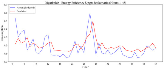
Figure 20.
Predictive performance of the final model under energy efficiency upgrade scenario in Diyarbakır: actual vs. predicted energy values.
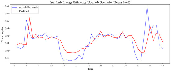
Figure 21.
Predictive performance of the final model under energy efficiency upgrade scenario in Istanbul: actual vs. predicted energy values.
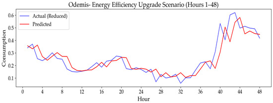
Figure 22.
Predictive performance of the final model under energy efficiency upgrade scenario in Odemis: actual vs. predicted energy values.
While Table 8 presents the numerical analysis of the final model’s performance, Figure 20, Figure 21 and Figure 22 visually illustrate its strong capacity to adapt to long-term positive trends under the Energy Efficiency Upgrade scenario. The plots clearly show the model’s ability to adjust to the lowered consumption baselines across all cities. For Istanbul (Figure 21), the visual evidence confirms the model’s pronounced adaptation, as the predicted line successfully shifts to track the new, lower consumption levels, directly corresponding to the significant RMSE decrease from 0.0436 to 0.0394. Similarly, the plots for Diyarbakır (Figure 20) and Odemis (Figure 22) visually demonstrate the model’s consistent adjustment, maintaining accuracy with minimal changes in RMSE. This strong capability to handle long-term efficiency changes is highly beneficial for Digital Twin applications, enabling them to deliver accurate forecasts of savings and monitor the impact of such initiatives.
Overall, the optimized enhanced stacked ensemble model exhibits a notable capacity for handling energy efficiency upgrades. This is evident in its strong ability to adapt to lowered consumption baselines and effectively track long-term positive trends, as demonstrated by the consistent or decreasing RMSE values across all cities. This capability proves highly beneficial for Digital Twin applications in sustainable energy management, as it empowers them to deliver precise savings forecasts and effectively monitor the long-term impact of efficiency initiatives.
4. Conclusions
This study comprehensively investigated the application of advanced Machine Learning techniques, specifically optimized stacked ensemble models, for high-fidelity energy consumption forecasting within a Simulated Digital Twin framework. Leveraging comprehensive datasets from Diyarbakır, Istanbul, and Odemis, our methodology systematically progressed from baseline models through sophisticated feature engineering and Bayesian Optimization to achieve accurate and robust predictive capabilities, which are crucial for dynamic and effective energy consumption forecasting.
Our experimental results clearly show the effective performance of the optimized enhanced stacked ensemble model. This approach consistently outperformed individual baseline algorithms and a standard stacking configuration. This is mainly because it effectively combines the strengths of different base learners while capturing complex time-based patterns through engineered lag features. Bayesian Optimization further improved accuracy, delivering optimal predictions across various household energy consumption profiles. This precise and reliable forecasting ability is important for scenario-based approaches, allowing for real-time monitoring, predictive analytics, and quick decision-making in energy management. Furthermore, testing and robustness analysis conducted under various Simulated Digital Twin scenarios provided important insights into the model’s real-world usability. The model showed remarkable resilience to common data quality issues (like missing data, outliers, sensor noise, and timestamp drift), maintaining high accuracy even when data was seriously corrupted. While the model adapted well to structural changes in consumption patterns, it struggled with sudden, large spikes. Odemis, in particular, showed the most significant deviations during these events. The model effectively handles appliance malfunctions and seamlessly adapts to new energy baselines after efficiency upgrades, proving its flexibility for smart energy projects. These findings confirm that the model can provide reliable insights even when real-world energy systems face data imperfections and dynamic changes.
The main contribution of this work is providing a systematic, high-performance forecasting model designed specifically for the demanding environment of real-world scenarios and their practical applications. Unlike traditional forecasting methods, our optimized stacked ensemble not only achieves forecasting accuracy but also shows an essential level of resilience to real-world anomalies and system changes. While this work supports active energy management, it also improves operational efficiency, enables predictive maintenance, and aids data-driven planning.
The SEF-SDT framework offers broad applications, contributing to the advancement of smarter and more sustainable energy systems. Its high-fidelity predictions enable active energy management in smart buildings by optimizing HVAC operations and lighting schedules, yielding measurable efficiency gains. For utility providers and grid operators, reliable short-term forecasts support demand-side management, ensuring grid stability and reducing blackout risks during peak demand. The framework’s detection of localized anomalies under the “Appliance Malfunction” scenario facilitates predictive maintenance by enabling timely fault identification and repair. Additionally, the SDT supports risk analysis and scenario planning in the absence of continuous real-time data, strengthening decision-making for future efficiency projects and system upgrades.
Despite the model’s strong performance, it is important to acknowledge some key limitations of this study. First, while the model is robust against many data quality issues and structural changes, it showed reduced performance and struggled to accurately predict extreme, sudden consumption spikes. A second limitation is that the model currently lacks an adaptive learning mechanism, which could be necessary to manage significant data drift over extended periods. Furthermore, the research was conducted within a Simulated Digital Twin environment. The performance and resilience of the model must be validated in a live, real-time system to confirm its full real-world applicability. Additionally, the research was conducted using datasets from three specific cities in Turkey (Diyarbakır, Istanbul, and Odemis). Therefore, the model’s generalizability to other countries with different climates, socio-cultural energy consumption habits, or grid infrastructures has not been directly validated. Finally, while the use of lagged features helps capture some temporal patterns, the model may not be robust enough to handle the significant, long-term shifts in energy consumption driven by seasonal changes, such as increased heating or cooling loads.
The current study’s findings provide a strong foundation for future research, particularly in the realm of real-time system integration and model adaptation. To directly address the limitation regarding real-time validation, future work will include deployment of the SEF-SDT framework in live smart grid projects. This will enable comprehensive assessment of model performance under operational conditions, allowing evaluation of prescriptive analytics, automated energy management, and real-time adaptation to dynamic consumption patterns. Such implementations will also provide insights into system integration challenges, data communication reliability, and practical scalability, further bridging the gap between simulation and operational deployment. A key future direction is the integration of our predictive models into a live Digital Twin platform, moving beyond the simulated environment. The primary objective is to validate their real-time performance and assess their capacity to enable prescriptive analytics and automated energy system optimization. To enhance the model’s long-term resilience and applicability in a dynamic environment, future work will also explore advanced online and adaptive learning mechanisms, such as stream-based learning algorithms or adaptive model retraining strategies. This approach would allow the model to automatically handle data drift and improve the prediction of extreme, sudden spikes in real-time. Finally, as a further research direction, federated learning may be explored to enable the models to learn collaboratively from data across multiple cities while maintaining data privacy and security.
Author Contributions
Conceptualization, A.O. and K.B.; methodology, A.O., K.B. and G.C.L.; software, A.A.H.K., O.T. and K.A.B.; validation, A.O., K.A.B. and O.T.; formal analysis, K.B.; investigation, A.O., K.B. and G.C.L.; resources, K.A.B., A.A.H.K. and O.T.; data curation, K.A.B., A.A.H.K. and O.T.; writing—original draft preparation, A.O.; writing—review and editing, K.B. and G.C.L.; visualization, O.T.; supervision, K.B. and G.C.L.; project administration, A.O. All authors have read and agreed to the published version of the manuscript.
Funding
This work was supported by a grant of the Ministry of Research, Innovation and Digitalization, project number PNRR-C9-I8-760089/23.05.2023, code CF31/14.11.2022.
Institutional Review Board Statement
Not applicable.
Informed Consent Statement
Not applicable.
Data Availability Statement
The original contributions presented in this study are included in the article. Further inquiries can be directed to the corresponding author.
Conflicts of Interest
The authors declare no conflicts of interest.
Abbreviations
The following abbreviations are used in this manuscript:
| SEF | Stacking Ensemble Forecasting |
| SDT | Simulated Digital Twin |
| SEF-SDT | Stacking Ensemble Forecasting via Simulated Digital Twin |
| ML | Machine Learning |
| AI | Artificial Intelligence |
| HVAC | Heating, Ventilation, and Air Conditioning |
| DT | Digital Twin |
| ANN | Artificial Neural Network |
| MLP | Multi-Layer Perceptron |
| KNR | K-Nearest Neighbors Regressor |
| SVM | K-Nearest Neighbors Regressor |
| SVR | Support Vector Regressor |
| RBF | Radial Basis Function |
| PSO | Particle Swarm Optimization |
| MPC | Model Predictive Control |
| ARIMA | AutoRegressive Integrated Moving Average |
| IQR | Interquartile Range |
| RMSE | Root Mean Squared Error |
| MAE | Mean Absolute Error |
| MAPE | Mean Absolute Percentage Error |
| R2 | Coefficient of Determination |
| BO | Bayesian Optimization |
| ETR | Extra Trees Regressor |
| GBR | Gradient Boosting Regressor |
| ABR | AdaBoost Regressor |
| RFR | Random Forest Regressor |
| UQ | Uncertainty Quantification |
| CV | Cross Validation |
| STD | Standard Deviation |
| kNN | k-Nearest Neighbors |
| PCA | Principal Component Analysis |
| API | Application Programming Interface |
Appendix A. Pseudocode the Complete Process
| FUNCTION EnergyConsumptionForecasting_Methodology: // 1. Data Collection INPUT: 3x Hourly Energy Consumption Datasets (Diyarbakır, Istanbul, Odemis) Each dataset covers [Start Date] to [End Date] Includes: Hourly Consumption (kWh), Calendar data OUTPUT: Raw Datasets {D_raw, I_raw, O_raw} // 2. Data Preprocessing FOR EACH D_raw_city IN {D_raw, I_raw, O_raw}: // Missing Value Imputation: E(t) = Median(E_window) // Outlier Handling: IF x NOT IN [Q1 − 1.5 × IQR, Q3 + 1.5 × IQR] THEN x = Median(E_window) OR Cap // Min-Max Normalization: E_norm(t) = (E(t) − E_min)/(E_max − E_min) OUTPUT: Preprocessed Datasets {D_proc, I_proc, O_proc} // 3. Feature Engineering FOR EACH D_proc_city IN {D_proc, I_proc, O_proc}: // Lagged Features: D_feat_city = D_proc_city + {E(t − 1), E(t − 24), E(t − 168)} OUTPUT: Featured Datasets {D_feat, I_feat, O_feat} // 4. Base Machine Learning Algorithm Pool BaseLearners_Pool = {AdaBoost, GradientBoosting, RandomForest, SVM, KNN, DecisionTree, LinearRegression, … (~15 diverse algorithms)} // 5. Data Splitting FOR EACH D_feat_city IN {D_feat, I_feat, O_feat}: (D_train_city, D_test_city) = Split(D_feat, test_size = 0.20) OUTPUT: Training Sets {D_train, I_train, O_train} Test Sets {D_test, I_test, O_test} // 6. Primary Performance Metric Metric: // 7. Initial Experiments & Base Learner Evaluation FOR EACH Learner in BaseLearners_Pool: FOR EACH (D_train_city, D_test_city) FROM Split Data: Train(Learner, D_train) Predictions = Predict(Learner, D_train_city) RMSE_score = Evaluate(Predictions, D_test_city_true_values, metric = RMSE) OUTPUT: All Base Learner RMSE Scores for each dataset // 8. Stacking Ensemble Generation (Initial Selection via Random Search) FOR EACH (D_train_city, D_test_city) FROM { (D_train, D_test), (I_train, I_test), (O_train, O_test) }: Stack_Architecture_Candidates = { BaseLearners: Subsets from BaseLearners_Pool, MetaLearner: A selected candidate algorithm } // Advanced Stacking Input: Meta-Learner_Input = [Original_Features, Base_Predictions_on_out_of_fold_data] Stack_Model_Initial = Optimize(Stack_Architecture_Candidates, (D_train_city, D_test_city), method = RandomSearch, objective = min(RMSE)) OUTPUT: Best Initial Stacking Ensemble Model // 9. Stacking Ensemble Hyperparameter Tuning (Bayesian Optimization) FOR EACH Stack_Model_Initial_city: Stack_Model_Optimized_city = Optimize(Stack_Model_Initial_city, (D_train_city, D_test_city), method = BayesianOptimization, objective = min(RMSE), acquisition_function = Expected_Improvement(EI)) OUTPUT: Optimized Stacking Ensemble Model_per city // 10. Scenario-Based Model Validation with SDT FOR EACH Stack_Model_Optimized_city: // Define Scenario Types and Generation Parameters based on operational conditions and data anomalies: // a. Standard Operational Conditions: Simulate // b. Outlier Robustness: Introduce specific outlier patterns (e.g., sudden spikes, sustained shifts) // c. Dynamic Consumption Patterns: Adjust and/or to reflect seasonal shifts or behavioral changes // d. Extreme Load or Low Demand: Simulate prolonged extreme high/low demand events FOR EACH Scenario_Type: Generate_Scenario_Data(Scenario_Type, D_test) Simulated_Predictions = Predict(Stack_Model_Optimized_city, Generated_Scenario_Data_features) Scenario_RMSE_score = Evaluate(Simulated_Predictions, Generated_Scenario_Data_true_values, metric = RMSE) OUTPUT: Model Robustness & Generalization Validation Report (RMSE scores for each scenario type per city) END FUNCTION |
References
- Ragupathi, C.; Dhanasekaran, S.; Vijayalakshmi, N.; Salau, A.O. Prediction of electricity consumption using an innovative deep energy predictor model for enhanced accuracy and efficiency. Energy Rep. 2024, 12, 5320–5337. [Google Scholar] [CrossRef]
- Cavus, M. Advancing power systems with renewable energy and intelligent technologies: A comprehensive review on grid transformation and integration. Electronics 2025, 14, 1159. [Google Scholar] [CrossRef]
- Javanmard, M.E.; Tang, Y.; Wang, Z.; Tontiwachwuthikul, P. Forecast energy demand, CO2 emissions and energy resource impacts for the transportation sector. Appl. Energy 2023, 338, 120830. [Google Scholar] [CrossRef]
- Chen, G.; Lu, S.; Zhou, S.; Tian, Z.; Kim, M.K.; Liu, J.; Liu, X. A Systematic Review of Building Energy Consumption Prediction: From Perspectives of Load Classification, Data-Driven Frameworks, and Future Directions. Appl. Sci. 2025, 15, 3086. [Google Scholar] [CrossRef]
- Henriques, L.; Castro, C.; Prata, F.; Leiva, V.; Venegas, R. Modeling Residential Energy Consumption Patterns with Machine Learning Methods Based on a Case Study in Brazil. Mathematics 2024, 12, 1961. [Google Scholar] [CrossRef]
- Dostmohammadi, M.; Zamani Pedram, M.; Hoseinzadeh, S.; Astiaso Garcia, D. A GA-stacking ensemble approach for forecasting energy consumption in a smart household: A comparative study of ensemble methods. J. Environ. Manag. 2024, 364, 121264. [Google Scholar] [CrossRef]
- Ali, Y.A.; Awwad, E.M.; Al-Razgan, M.; Maarouf, A. Hyperparameter Search for Machine Learning Algorithms for Optimizing the Computational Complexity. Processes 2023, 11, 349. [Google Scholar] [CrossRef]
- Henzel, J.; Wróbel, Ł.; Fice, M.; Sikora, M. Energy Consumption Forecasting for the Digital-Twin Model of the Building. Energies 2022, 15, 4318. [Google Scholar] [CrossRef]
- Mystakidis, A.; Koukaras, P.; Tsalikidis, N.; Ioannidis, D.; Tjortjis, C. Energy Forecasting: A Comprehensive Review of Techniques and Technologies. Energies 2024, 17, 1662. [Google Scholar] [CrossRef]
- Tsegaye, S.; Sanjeevikumar, P.; Tjernberg, L.B.; Fante, K.A. Short-term energy forecasting using deep neural networks: Prospects and challenges. J. Eng. 2024, 2024, e70022. [Google Scholar] [CrossRef]
- Yang, Y.; Li, Y.; Cheng, L.; Yang, S. Short-Term Wind Power Prediction Based on a Modified Stacking Ensemble Learning Algorithm. Sustainability 2024, 16, 5960. [Google Scholar] [CrossRef]
- Cao, Y.; Liu, G.; Sun, J.; Bavirisetti, D.P.; Xiao, G. PSO-Stacking improved ensemble model for campus building energy consumption forecasting based on priority feature selection. J. Build. Eng. 2023, 72, 106589. [Google Scholar] [CrossRef]
- Luo, S.; Wang, B.; Gao, Q.; Wang, Y.; Pang, X. Stacking integration algorithm based on CNN-BiLSTM-Attention with XGBoost for short-term electricity load forecasting. Energy Rep. 2024, 12, 2676–2689. [Google Scholar] [CrossRef]
- Olu-Ajayi, R.; Alaka, H.; Sulaimon, I.; Sunmola, F.; Ajayi, S. Building energy consumption prediction for residential buildings using deep learning and other machine learning techniques. J. Build. Eng. 2022, 45, 103406. [Google Scholar] [CrossRef]
- Reddy, S.; Akashdeep, S.; Harshvardhan, R.; Kamath, S. Stacking Deep learning and Machine learning models for short-term energy consumption forecasting. Adv. Eng. Inform. 2022, 52, 101542. [Google Scholar] [CrossRef]
- Chen, B.; Wang, Y. Short-term electric load forecasting of integrated energy system considering nonlinear synergy between different loads. IEEE Access 2021, 9, 43562–43573. [Google Scholar] [CrossRef]
- Sghiri, A.; Gallab, M.; Merzouk, S.; Assoul, S. Leveraging Digital Twins for Enhancing Building Energy Efficiency: A Literature Review of Applications, Technologies, and Challenges. Buildings 2025, 15, 498. [Google Scholar] [CrossRef]
- Boschert, S.; Rosen, R. Digital Twin—The Simulation Aspect. In Mechatronic Futures; Hehenberger, P., Bradley, D., Eds.; Springer: Cham, Switzerland, 2016; pp. 59–74. [Google Scholar]
- Barricelli, B.R.; Casiraghi, E.; Fogli, D. A Survey on Digital Twin: Definitions, Characteristics, Applications, and Design Implications. IEEE Access 2019, 7, 167653–167670. [Google Scholar] [CrossRef]
- Li, C.; Lu, P.; Zhu, W.; Zhu, H.; Zhang, X. Intelligent Monitoring Platform and Application for Building Energy Using Information Based on Digital Twin. Energies 2023, 16, 6839. [Google Scholar] [CrossRef]
- You, M.; Wang, Q.; Sun, H.; Castro, I.; Jiang, J. Digital twins based day-ahead integrated energy system scheduling under load and renewable energy uncertainties. Appl. Energy 2022, 305, 117899. [Google Scholar] [CrossRef]
- Hosamo, H.; Hosamo, M.H.; Nielsen, H.K.; Svennevig, P.R.; Svidt, K. Digital Twin of HVAC system (HVACDT) for multiobjective optimization of energy consumption and thermal comfort based on BIM framework with ANN-MOGA. Adv. Build. Energy Res. 2022, 17, 125–171. [Google Scholar] [CrossRef]
- Clausen, A.; Arendt, K.; Johansen, A.; Jacobsen, J.M.; Rysgaard, J.; Christensen, J.D. A digital twin framework for improving energy efficiency and occupant comfort in public and commercial buildings. Energy Inform. 2021, 4 (Suppl. 2), 40. [Google Scholar] [CrossRef]
- Liu, Y.; Li, B.; Liang, H. Building Electricity Prediction Using BILSTM-RF-XGBOOST Hybrid Model with Improved Hyperparameters Based on Bayesian Algorithm. Electronics 2025, 14, 2287. [Google Scholar] [CrossRef]
- Guo, F.; Mo, H.; Wu, J.; Pan, L.; Zhou, H.; Zhang, Z.; Li, L.; Huang, F. A Hybrid Stacking Model for Enhanced Short-Term Load Forecasting. Electronics 2024, 13, 2719. [Google Scholar] [CrossRef]
- Meng, F.; Wang, X. Digital twin for intelligent probabilistic short term load forecasting in solar based smart grids using shark algorithm. Sol. Energy 2023, 262, 111870. [Google Scholar] [CrossRef]
- Lee, J.; Park, E.; Lee, S. Development of a Hybrid Modeling Framework for the Optimal Operation of Microgrids. Energies 2025, 18, 2102. [Google Scholar] [CrossRef]
- Wen, Q.; Liu, Y. Feature engineering and selection for prosumer electricity consumption and production forecasting: A comprehensive framework. Appl. Energy 2025, 381, 125176. [Google Scholar] [CrossRef]
- Hastie, T.; Tibshirani, R.; Friedman, J. The Elements of Statistical Learning: Data Mining, Inference, and Prediction; Springer: Berlin/Heidelberg, Germany, 2009. [Google Scholar]
- Ansari, S.; Nassif, A.B. A Comprehensive Study of Regression Analysis and the Existing Techniques. In Proceedings of the 2022 Advances in Science and Engineering Technology International Conferences (ASET), Dubai, United Arab Emirates, 21–24 February 2022. [Google Scholar]
- Breiman, L. Random Forests. Mach. Learn. 2001, 45, 5–32. [Google Scholar] [CrossRef]
- Mienye, I.D.; Sun, Y. A Survey of Ensemble Learning: Concepts, Algorithms, Applications, and Prospects. IEEE Access 2022, 10, 99129–99149. [Google Scholar] [CrossRef]
- Geurts, P.; Ernst, D.; Wehenkel, L. Extremely randomized trees. Mach. Learn. 2006, 63, 3–42. [Google Scholar] [CrossRef]
- Liashchynskyi, P.; Liashchynskyi, P. Grid Search, Random Search, Genetic Algorithm: A Big Comparison for NAS. arXiv 2019, arXiv:1912.06059. [Google Scholar] [CrossRef]
- Shahriari, B.; Swersky, K.; Wang, Z.; Adams, R.P.; de Freitas, N. Taking the human out of the loop: A review of Bayesian optimization. Proc. IEEE 2016, 104, 148–175. [Google Scholar] [CrossRef]
- El-Kenawy, E.-S.M.; Mirjalili, S.; Ghoneim, S.S.; Eid, M.M.; El-Said, M.; Khan, Z.S.; Ibrahim, A. Advanced ensemble model for solar radiation forecasting using Sine Cosine Algorithm and Newton’s Laws. IEEE Access 2021, 9, 115750–115765. [Google Scholar] [CrossRef]
- Ismail, F.B.; Al-Faiz, H.; Hasini, H.; Al-Bazi, A.; Kazem, H.A. A comprehensive review of the dynamic applications of the digital twin technology across diverse energy sectors. Energy Strategy Rev. 2024, 52, 101334. [Google Scholar] [CrossRef]
- Rahmani-Sane, G.; Azad, S.; Ameli, M.T.; Haghani, S. The Applications of Artificial Intelligence and Digital Twin in Power Systems: An In-Depth Review. IEEE Access 2025, 13, 108573–108608. [Google Scholar] [CrossRef]


Disclaimer/Publisher’s Note: The statements, opinions and data contained in all publications are solely those of the individual author(s) and contributor(s) and not of MDPI and/or the editor(s). MDPI and/or the editor(s) disclaim responsibility for any injury to people or property resulting from any ideas, methods, instructions or products referred to in the content. |
© 2025 by the authors. Licensee MDPI, Basel, Switzerland. This article is an open access article distributed under the terms and conditions of the Creative Commons Attribution (CC BY) license (https://creativecommons.org/licenses/by/4.0/).