
Impact of Key DMD Parameters on Modal Analysis of High-Reynolds-Number Flow Around an Idealized Ground Vehicle


Abstract
1. Introduction
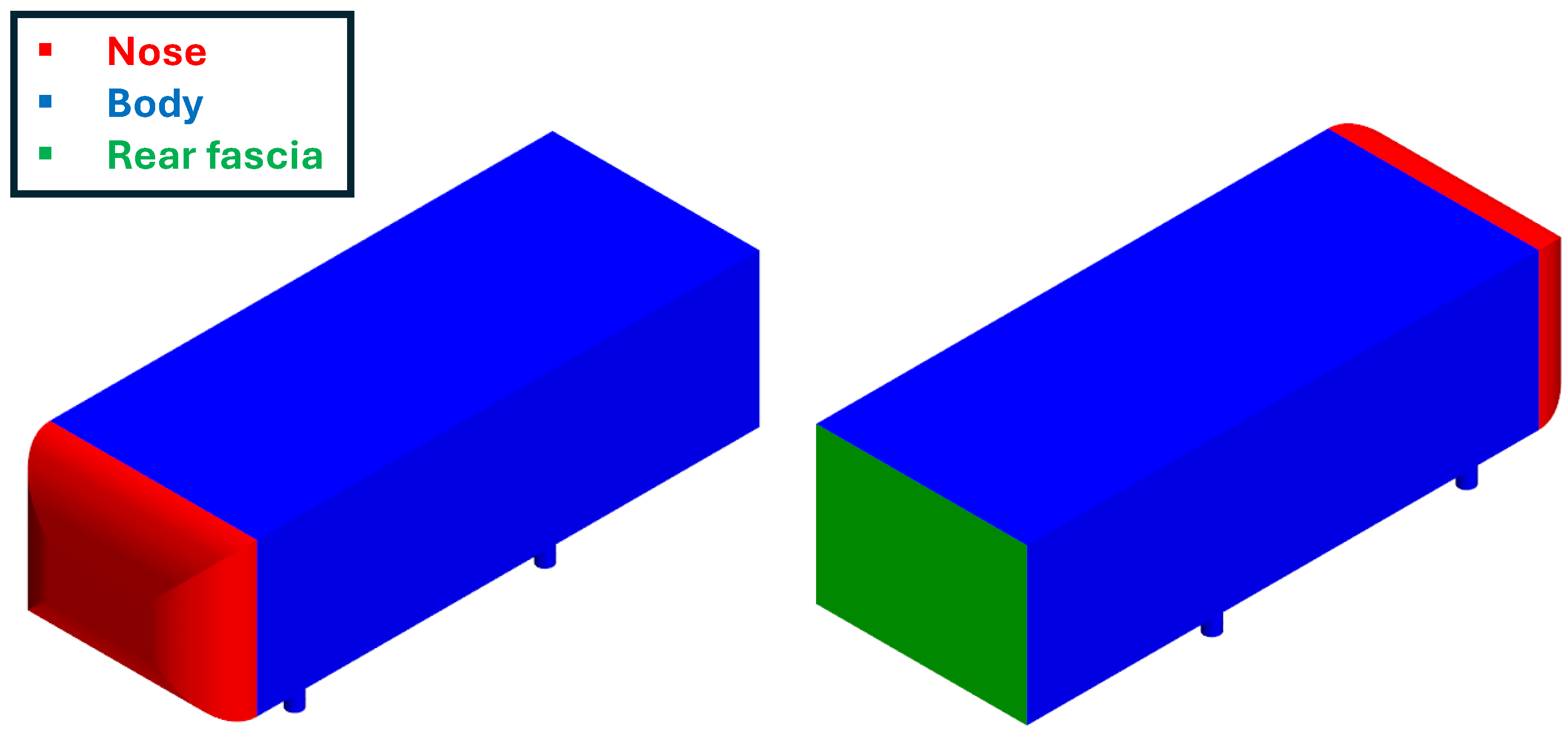
2. Numerical Setup
3. DMD Algorithm
4. Numerical Validation
4.1. Aerodynamic Coefficients
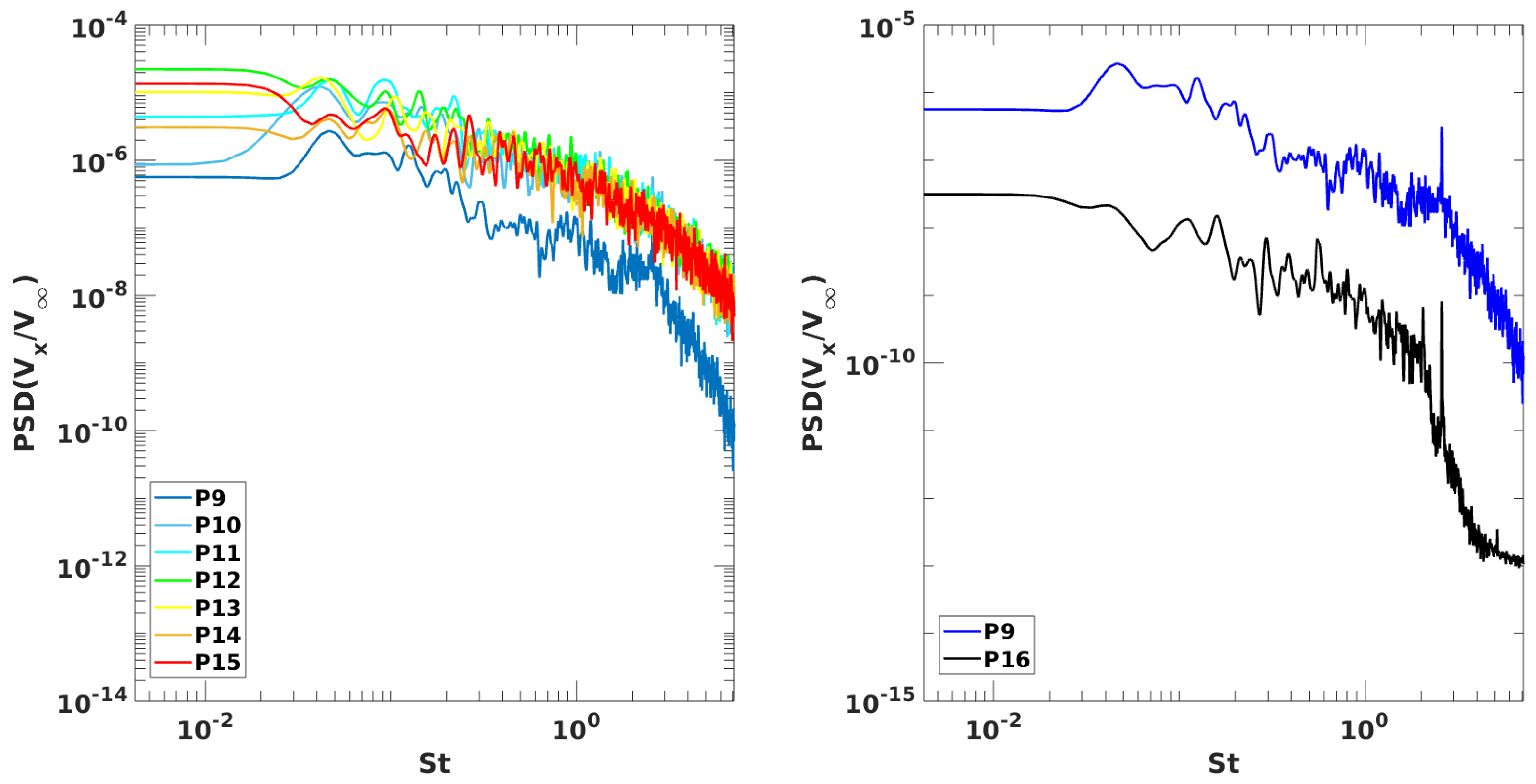
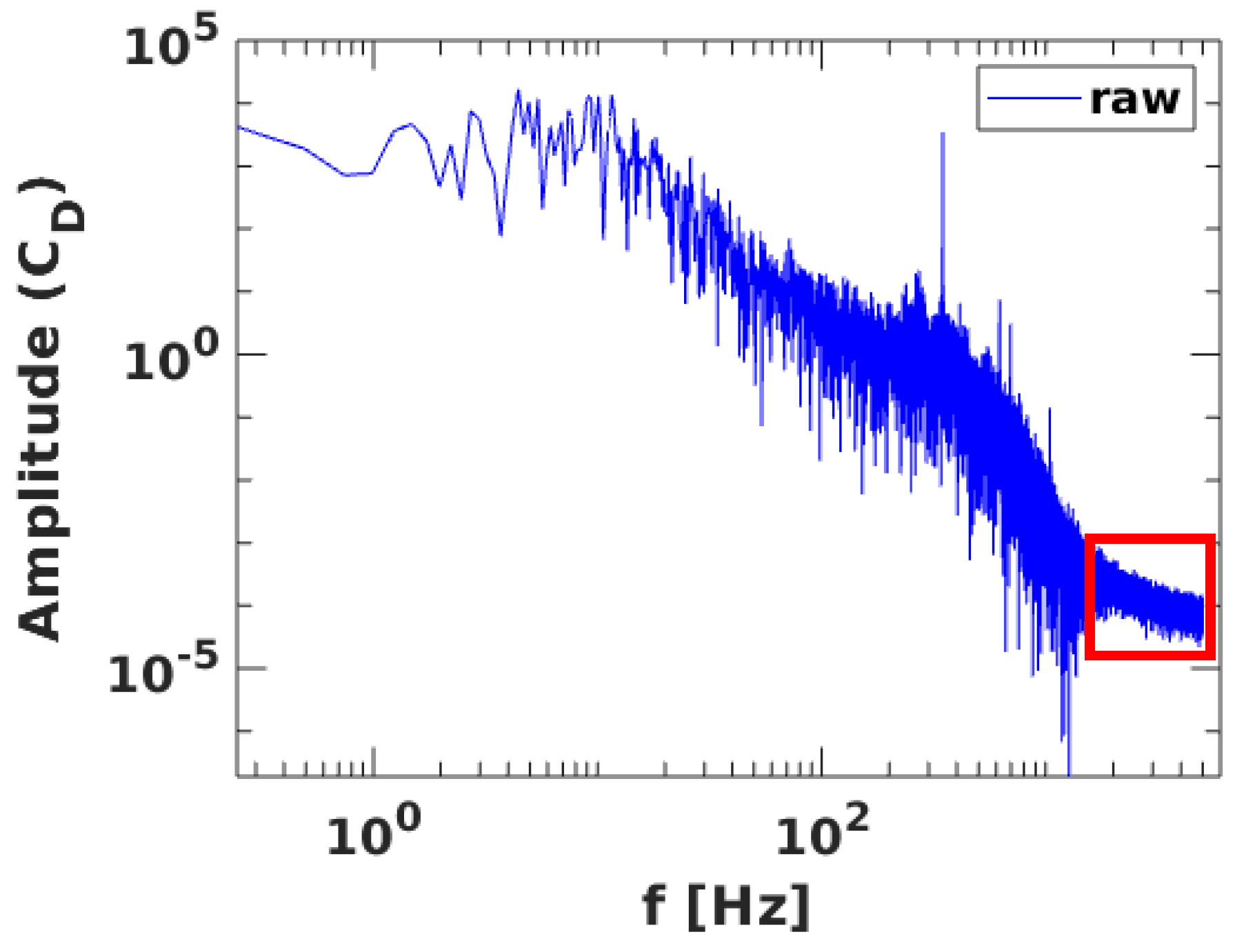
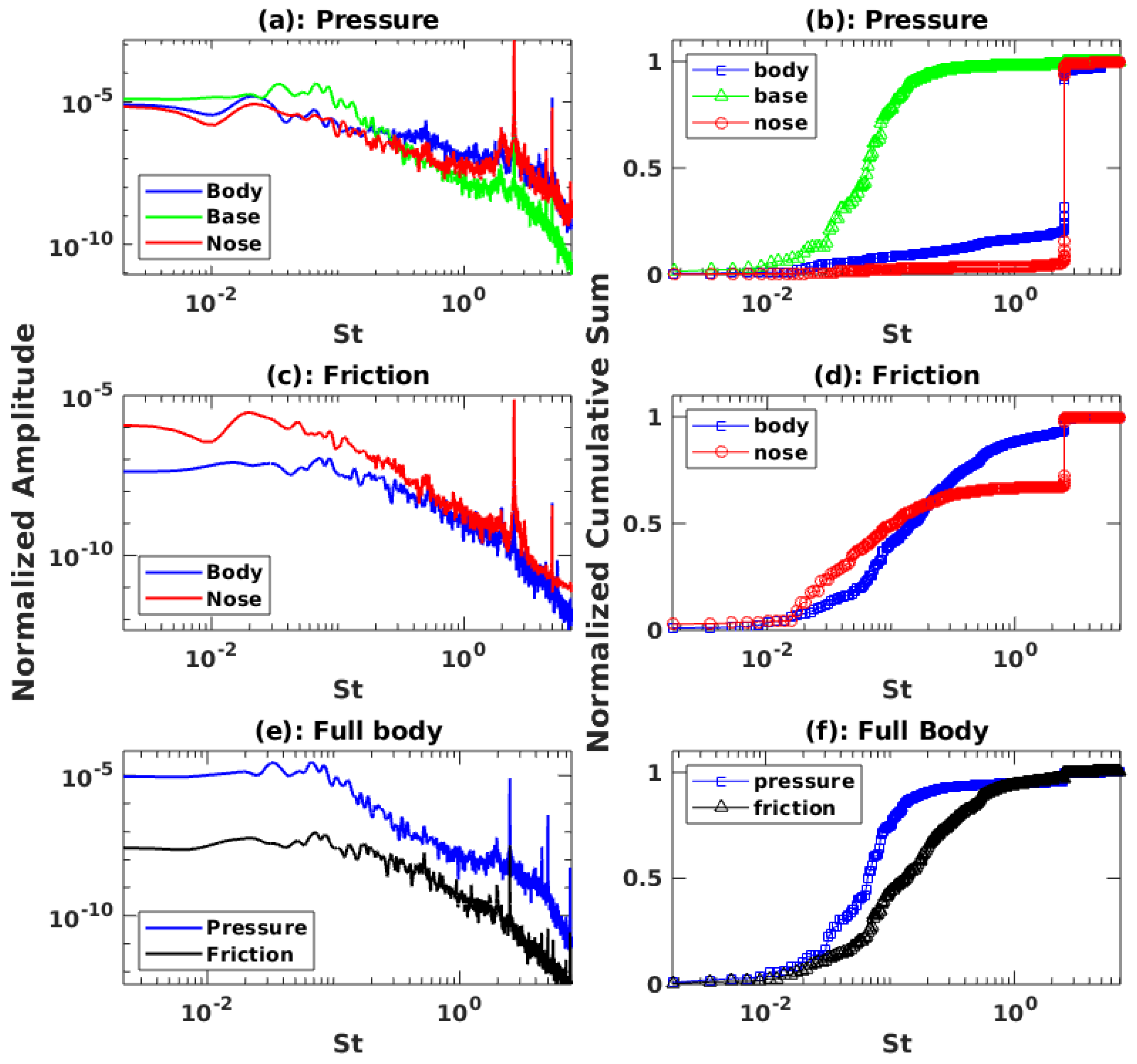
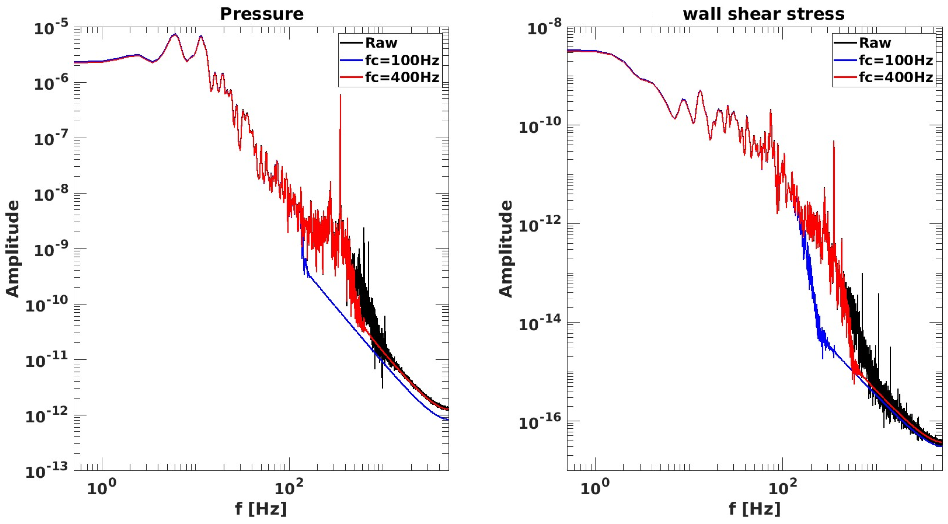
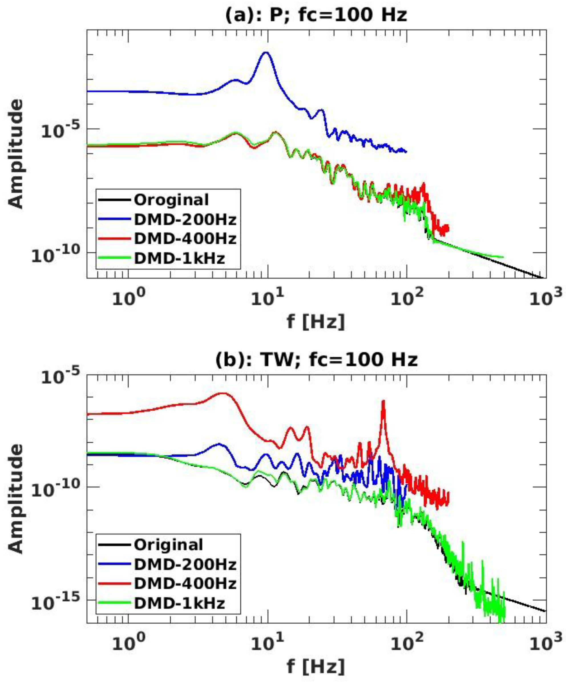
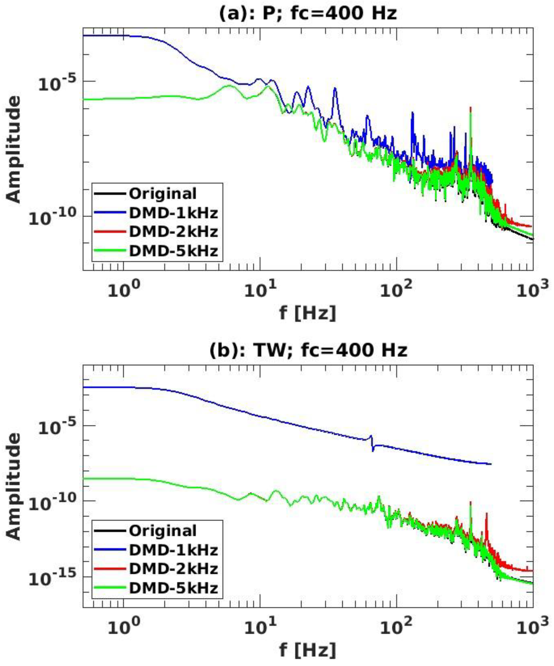
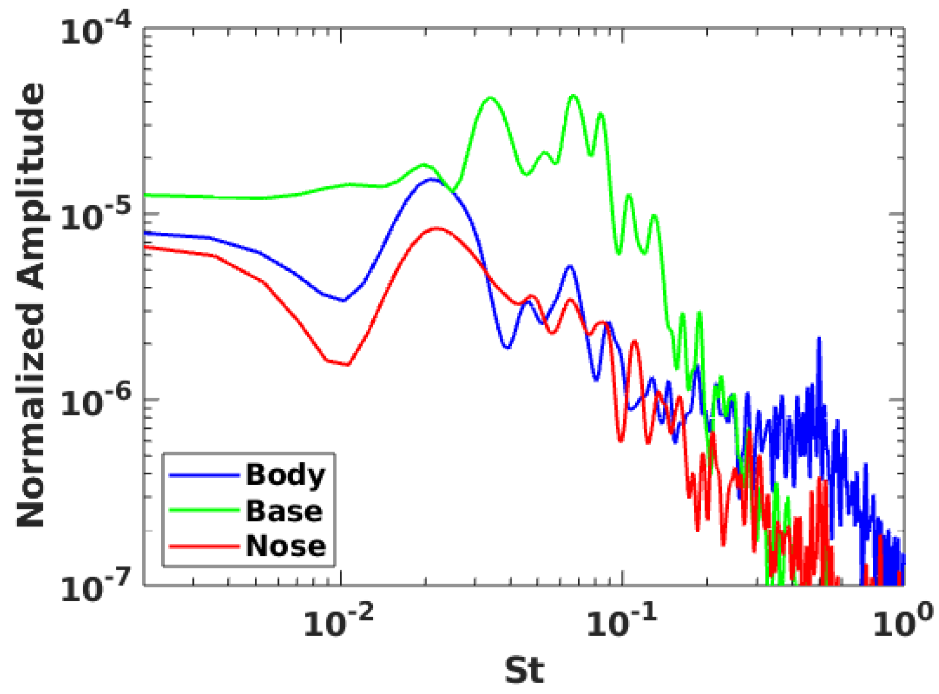
4.2. Signal Spectrum
5. Results and Discussion
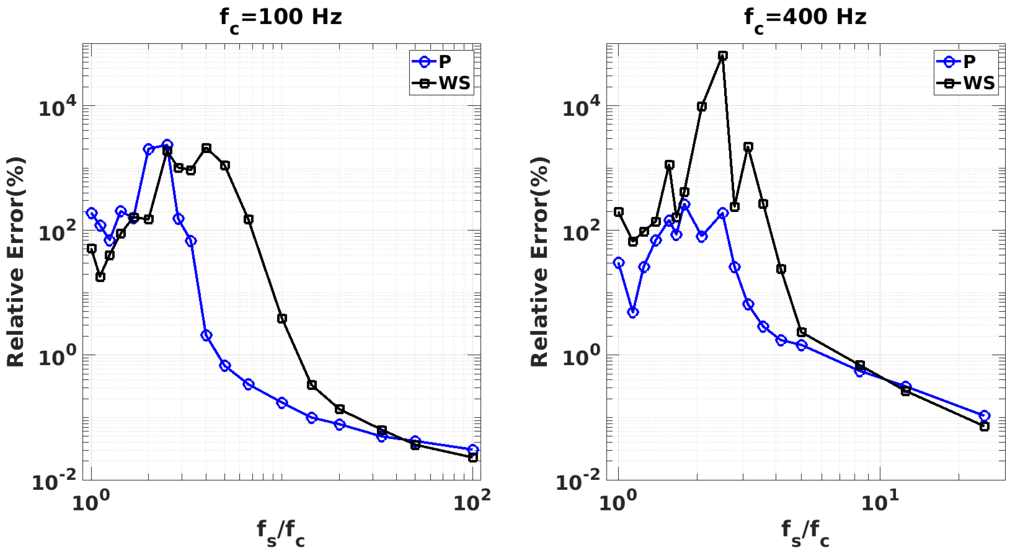
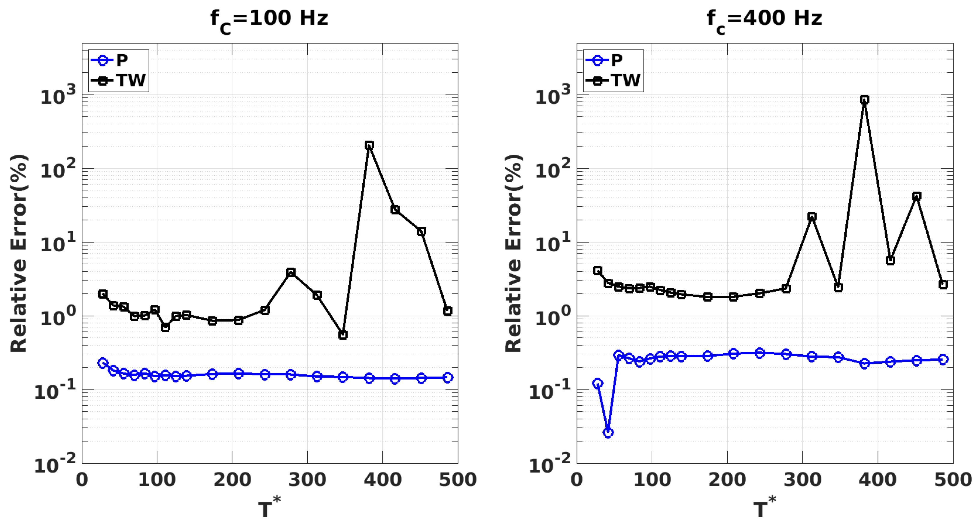
5.1. Drag Force Sensitivity to Sampling Frequency and Period
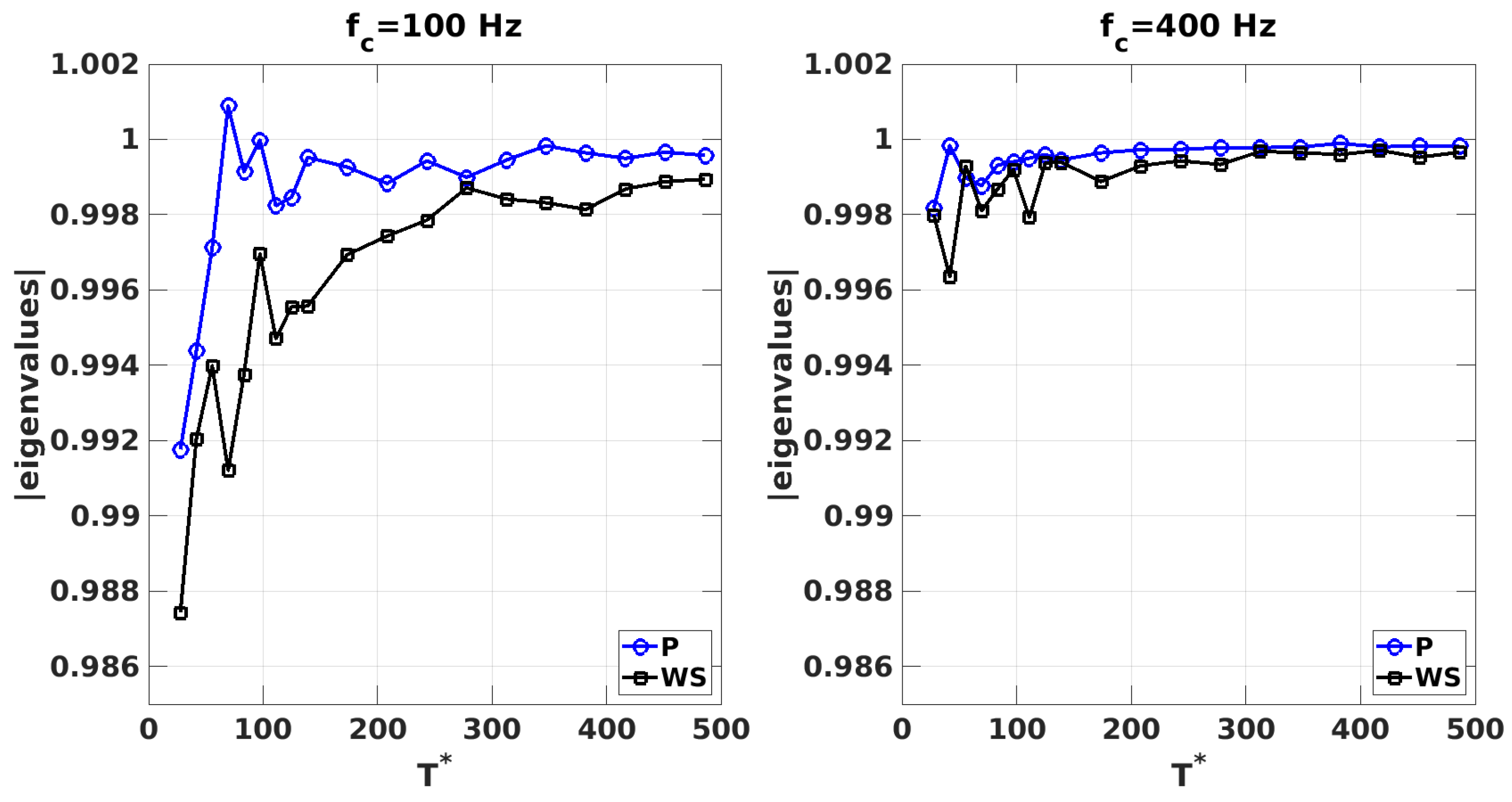
5.2. DMD Convergence Criterion
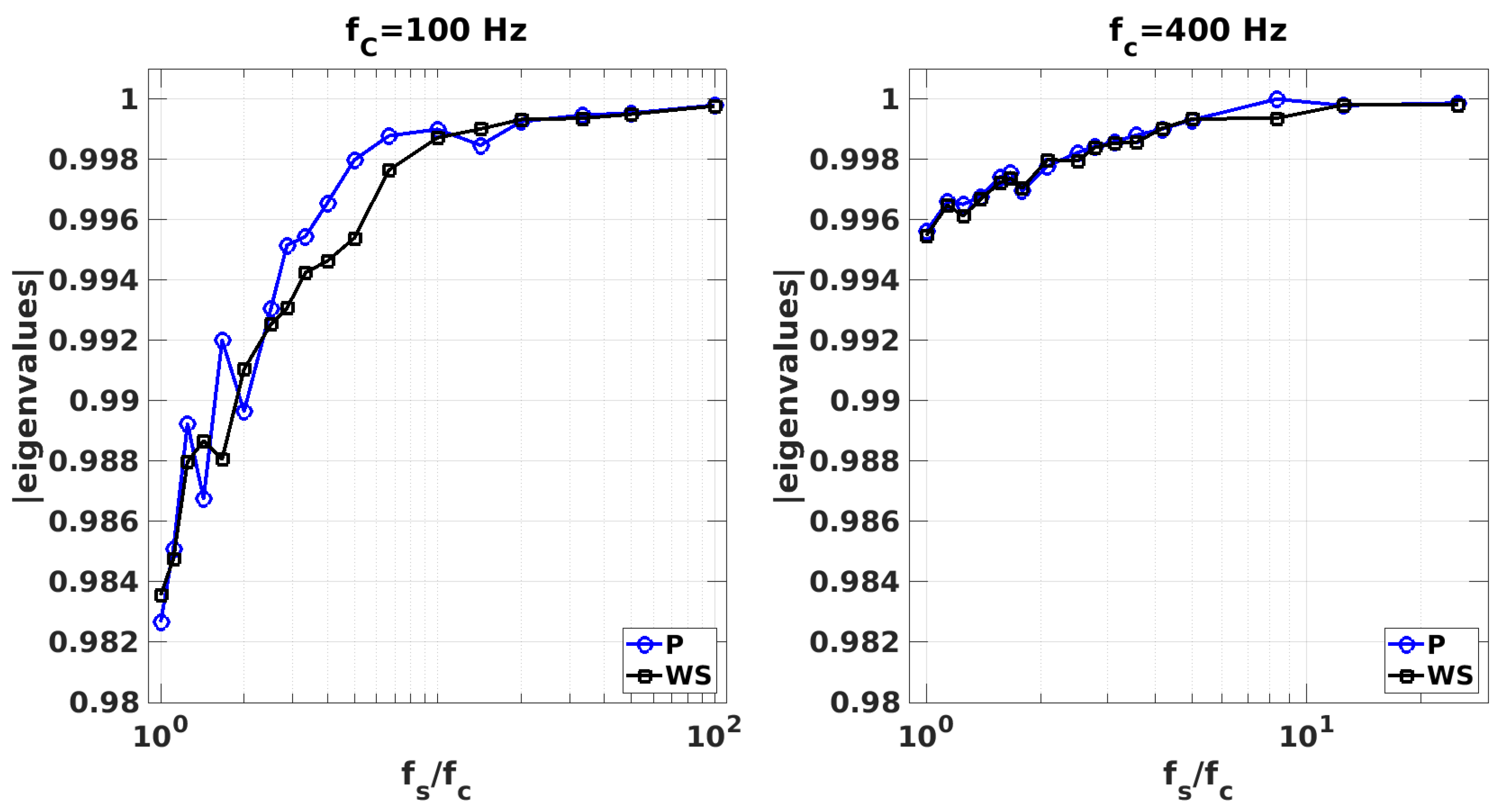
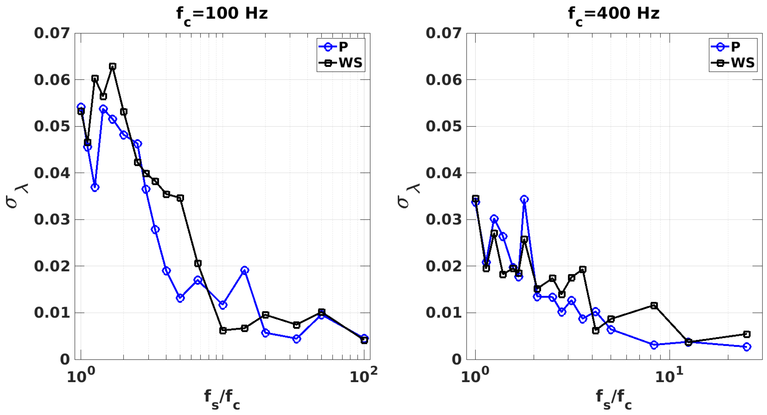
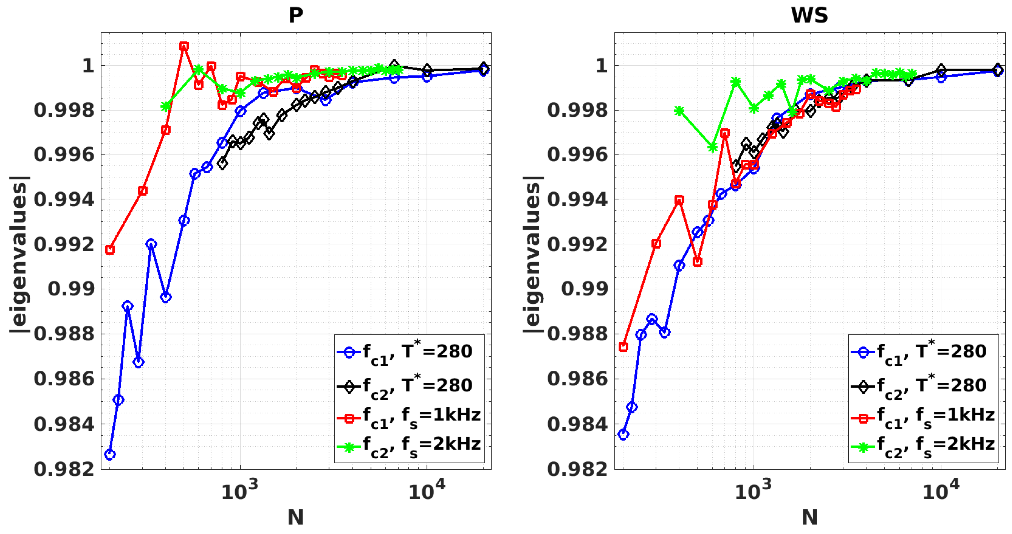
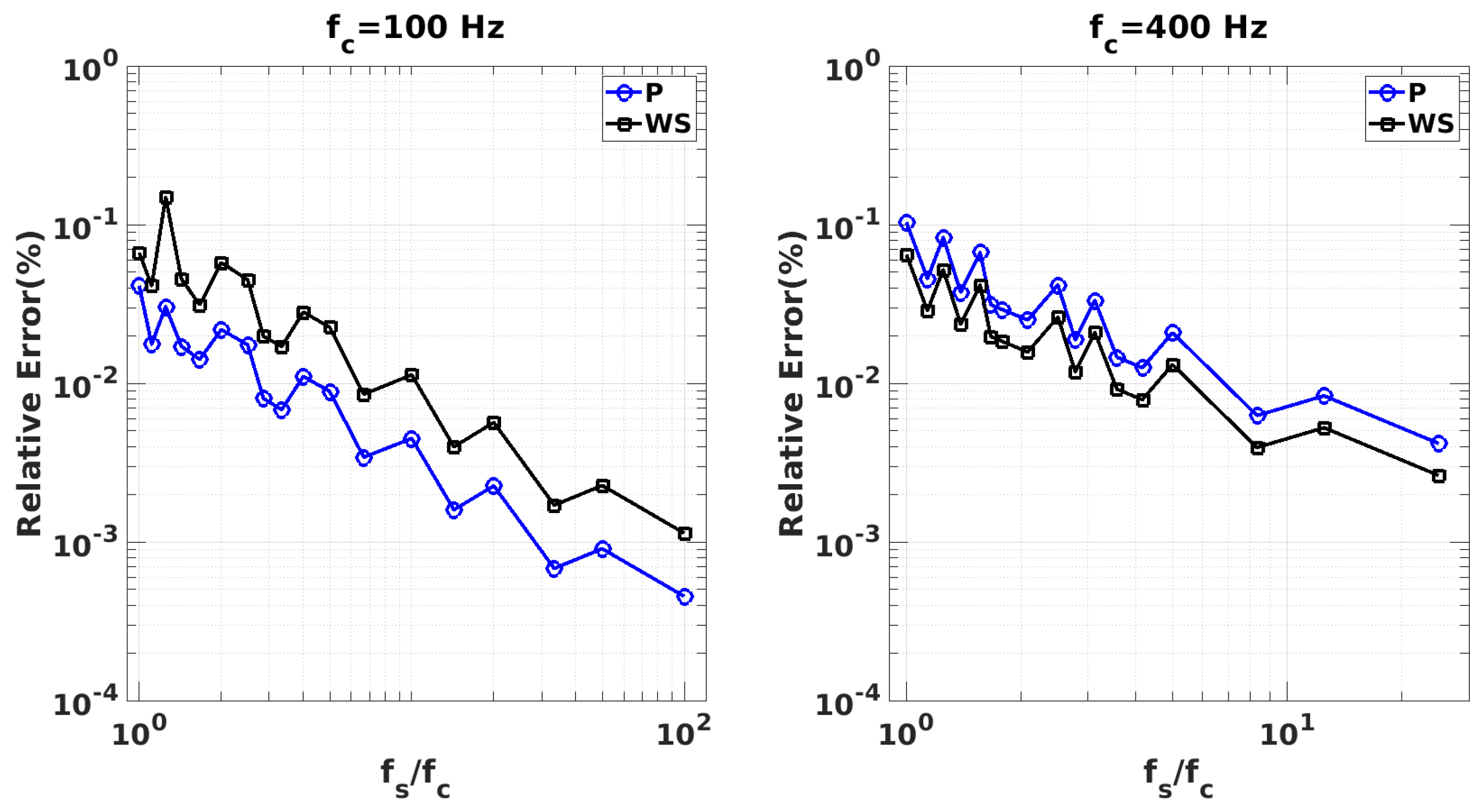
5.2.1. Convergence of Sampling Frequency
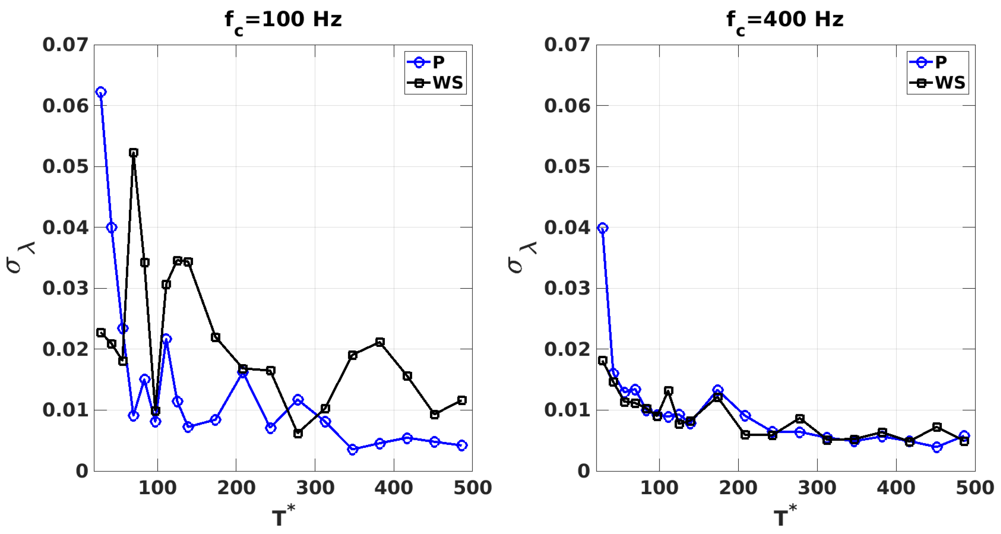
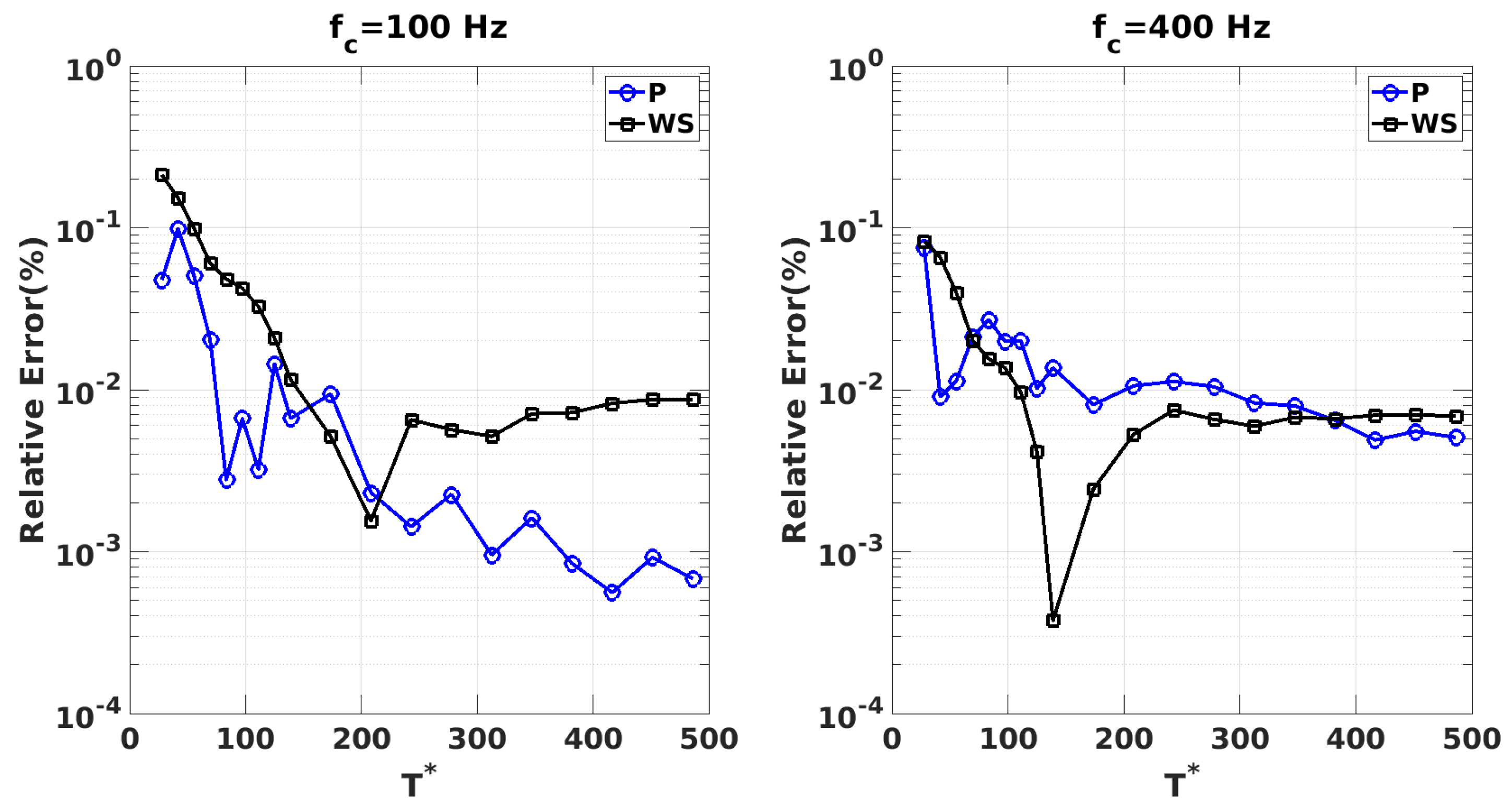
5.2.2. Convergence of Sampling Period
5.3. Mean-Subtracted DMD
6. Conclusions
Author Contributions
Funding
Institutional Review Board Statement
Informed Consent Statement
Data Availability Statement
Conflicts of Interest
References
- Townsend, A.A. The Structure of Turbulent Shear Flow Camb; Cambridge University Press: Cambridge, UK, 1956; Chapter 6. [Google Scholar]
- Taylor, G.I. The spectrum of turbulence. Proc. R. Soc. Lond. Ser. A-Math. Phys. Sci. 1938, 164, 476–490. [Google Scholar] [CrossRef]
- Klotz, L.; Pavlenko, A.; Wesfreid, J. Experimental measurements in plane Couette–Poiseuille flow: Dynamics of the large-and small-scale flow. J. Fluid Mech. 2021, 912, A24. [Google Scholar] [CrossRef]
- Lumley, J.L. The Structure of Inhomogeneous Turbulent Flows. Atmospheric Turbulence and RadioWave Propagation. Nauka. 1967, pp. 166–178. Available online: https://cir.nii.ac.jp/crid/1574231874542771712 (accessed on 7 January 2025).
- Gordeyev, S.V.; Thomas, F.O. Coherent structure in the turbulent planar jet. Part 1. Extraction of proper orthogonal decomposition eigenmodes and their self-similarity. J. Fluid Mech. 2000, 414, 145–194. [Google Scholar] [CrossRef]
- Meyer, K.E.; Pedersen, J.M.; Özcan, O. A turbulent jet in crossflow analysed with proper orthogonal decomposition. J. Fluid Mech. 2007, 583, 199–227. [Google Scholar] [CrossRef]
- Ravindran, S.S. A reduced-order approach for optimal control of fluids using proper orthogonal decomposition. Int. J. Numer. Methods Fluids 2000, 34, 425–448. [Google Scholar] [CrossRef]
- Noack, B.R.; Afanasiev, K.; Morzyński, M.; Tadmor, G.; Thiele, F. A hierarchy of low-dimensional models for the transient and post-transient cylinder wake. J. Fluid Mech. 2003, 497, 335–363. [Google Scholar] [CrossRef]
- Alonso, D.; Vega, J.; Velazquez, A. Reduced-order model for viscous aerodynamic flow past an airfoil. AIAA J. 2010, 48, 1946–1958. [Google Scholar] [CrossRef]
- Morlet, J. A Decomposition of hardy into square integrable wavelets of constant shape. SIAM J. Math Anal. 1980, 15, 723–736. [Google Scholar]
- Farge, M.; Rabreau, G. Wavelet transform to analyze coherent structures in two-dimensional turbulent flows. In Proceedings of the Scaling, Fractals and Nonlinear Variability in Geophysics 1, Paris, France, June 1988. [Google Scholar]
- Farge, M. Wavelet transforms and their applications to turbulence. Annu. Rev. Fluid Mech. 1992, 24, 395–458. [Google Scholar] [CrossRef]
- Ballouz, E.; Dawson, S.T.; Bae, H.J. Transient growth of wavelet-based resolvent modes in the buffer layer of wall-bounded turbulence. J. Phys. Conf. Ser. 2024, 2753, 012002. [Google Scholar] [CrossRef]
- Kang, D.; Lee, S.; Brouzet, D.; Lele, S.K. Wavelet-based pressure decomposition for airfoil noise in low-Mach number flows. Phys. Fluids 2023, 35, 075112. [Google Scholar] [CrossRef]
- Alam, J.M. Wavelet Transforms and Machine Learning Methods for the Study of Turbulence. Fluids 2023, 8, 224. [Google Scholar] [CrossRef]
- Zheng, Y.; Zhang, D.; Wang, T.; Rinoshika, H.; Rinoshika, A. A hybrid two-dimensional orthogonal wavelet multiresolution and proper orthogonal decomposition technique for the analysis of turbulent wake flow. Ocean Eng. 2022, 264, 112547. [Google Scholar] [CrossRef]
- Schmid, P.J. Dynamic mode decomposition of numerical and experimental data. J. Fluid Mech. 2010, 656, 5–28. [Google Scholar] [CrossRef]
- Hemati, M.; Deem, E.; Williams, M.; Rowley, C.W.; Cattafesta, L.N. Improving separation control with noise-robust variants of dynamic mode decomposition. In Proceedings of the 54th AIAA Aerospace Sciences Meeting, San Diego, CA, USA, 4–8 January 2016; p. 1103. [Google Scholar]
- Le Clainche, S.; Vega, J.M. Higher order dynamic mode decomposition to identify and extrapolate flow patterns. Phys. Fluids 2017, 29, 084102. [Google Scholar] [CrossRef]
- Sayadi, T.; Schmid, P.J.; Nichols, J.W.; Moin, P. Reduced-order representation of near-wall structures in the late transitional boundary layer. J. Fluid Mech. 2014, 748, 278–301. [Google Scholar] [CrossRef]
- Yu, M.; Huang, W.X.; Xu, C.X. Data-driven construction of a reduced-order model for supersonic boundary layer transition. J. Fluid Mech. 2019, 874, 1096–1114. [Google Scholar] [CrossRef]
- Ma, Z.; Yu, J.; Xiao, R. Data-driven reduced order modeling for parametrized time-dependent flow problems. Phys. Fluids 2022, 34, 075109. [Google Scholar] [CrossRef]
- Schmid, P.J. Dynamic mode decomposition and its variants. Annu. Rev. Fluid Mech. 2022, 54, 225–254. [Google Scholar] [CrossRef]
- Ikeda, J.; Matsumoto, D.; Tsubokura, M.; Uchida, M.; Hasegawa, T.; Kobayashi, R. Dynamic mode decomposition of flow around a full-scale road vehicle using unsteady CFD. In Proceedings of the 34th AIAA Applied Aerodynamics Conference, Washington, DC, USA, 13–17 June 2016; p. 3727. [Google Scholar]
- Ikeda, J.; Tsubokura, M.; Hasegawa, T.; Kobayashi, R. Effect of Unsteady Aerodynamics on Drivability of Road Vehicles using LES and Modal Analysis. In Proceedings of the 35th AIAA Applied Aerodynamics Conference, Denver, CO, USA, 5–9 June 2017; p. 3907. [Google Scholar]
- Edwige, S.; Eulalie, Y.; Gilotte, P.; Mortazavi, I. Wake flow analysis and control on a 47 slant angle Ahmed body. Int. J. Numer. Methods Heat Fluid Flow 2018, 28, 1061–1079. [Google Scholar] [CrossRef]
- Evstafyeva, O.; Morgans, A.; Dalla Longa, L. Simulation and feedback control of the Ahmed body flow exhibiting symmetry breaking behaviour. J. Fluid Mech. 2017, 817, R2. [Google Scholar] [CrossRef]
- Dalla Longa, L.; Evstafyeva, O.; Morgans, A. Simulations of the bi-modal wake past three-dimensional blunt bluff bodies. J. Fluid Mech. 2019, 866, 791–809. [Google Scholar] [CrossRef]
- Ahani, H.; Nielsen, J.; Uddin, M. The Proper Orthogonal and Dynamic Mode Decomposition of Wake Behind a Fastback DrivAer Model; Technical Report; SAE Technical Paper: Warrendale, PA, USA, 2022. [Google Scholar]
- Heft, A.I.; Indinger, T.; Adams, N.A. Experimental and numerical investigation of the DrivAer model. In Proceedings of the Fluids Engineering Division Summer Meeting. American Society of Mechanical Engineers, Rio Grande, PR, USA, 8–12 July 2012; Volume 44755, pp. 41–51. [Google Scholar]
- Siddiqui, N.A.; Agelin-Chaab, M. Experimental investigation of the flow features around an elliptical Ahmed body. Phys. Fluids 2022, 34, 105119. [Google Scholar] [CrossRef]
- Misar, A.; Tison, N.A.; Korivi, V.M.; Uddin, M. Application of the DMD approach to high-Reynolds-number flow over an idealized ground vehicle. Vehicles 2023, 5, 656–681. [Google Scholar] [CrossRef]
- Chen, K.K.; Tu, J.H.; Rowley, C.W. Variants of dynamic mode decomposition: Boundary condition, Koopman, and Fourier analyses. J. Nonlinear Sci. 2012, 22, 887–915. [Google Scholar] [CrossRef]
- Li, C.Y.; Chen, Z.; Tse, T.K.; Weerasuriya, A.U.; Zhang, X.; Fu, Y.; Lin, X. A parametric and feasibility study for data sampling of the dynamic mode decomposition: Range, resolution, and universal convergence states. Nonlinear Dyn. 2022, 107, 3683–3707. [Google Scholar] [CrossRef]
- Lahaye, A.; Leroy, A.; Kourta, A. Aerodynamic characterisation of a square back bluff body flow. Int. J. Aerodyn. 2014, 4, 43–60. [Google Scholar] [CrossRef]
- Muld, T.W.; Efraimsson, G.; Henningson, D.S. Mode decomposition on surface-mounted cube. Flow Turbul. Combust. 2012, 88, 279–310. [Google Scholar] [CrossRef]
- Travin, A.K.; Shur, M.L.; Spalart, P.R.; Strelets, M.K. Improvement of delayed detached-eddy simulation for LES with wall modelling. In Proceedings of the ECCOMAS CFD 2006: Proceedings of the European Conference on Computational Fluid Dynamics, Egmond aan Zee, The Netherlands, 5–8 September 2006; Delft University of Technology: Delft, The Netherlands, 2006. European Community on Computational Methods. [Google Scholar]
- Menter, F.R. Two-equation eddy-viscosity turbulence models for engineering applications. AIAA J. 1994, 32, 269–289. [Google Scholar] [CrossRef]
- Bounds, C.P.; Rajasekar, S.; Uddin, M. Development of a numerical investigation framework for ground vehicle platooning. Fluids 2021, 6, 404. [Google Scholar] [CrossRef]
- Ashton, N.; West, A.; Lardeau, S.; Revell, A. Assessment of RANS and DES methods for realistic automotive models. Comput. Fluids 2016, 128, 1–15. [Google Scholar] [CrossRef]
- Guilmineau, E.; Deng, G.; Leroyer, A.; Queutey, P.; Wackers, J.; Visonneau, M. Assessment of RANS and DES methods for the Ahmed body. In Proceedings of the ECCOMAS Congress 2016-VII European Congress on Computational Methods in Applied Sciences and Engineering, Crete, Greece, 5–10 June 2016. [Google Scholar]
- Fu, C.; Bounds, C.P.; Selent, C.; Uddin, M. Turbulence modeling effects on the aerodynamic characterizations of a NASCAR Generation 6 racecar subject to yaw and pitch changes. Proc. Inst. Mech. Eng. Part D J. Automob. Eng. 2019, 233, 3600–3620. [Google Scholar] [CrossRef]
- Misar, A.; Davis, P.; Uddin, M. On the Effectiveness of Scale-Averaged RANS and Scale-Resolved IDDES Turbulence Simulation Approaches in Predicting the Pressure Field over a NASCAR Racecar. Fluids 2023, 8, 157. [Google Scholar] [CrossRef]
- Spalart, P.R. Comments on the Feasibility of LES for Wings and on the Hybrid RANS/LES Approach. In Proceedings of the First AFOSR International Conference on DNS/LES, Ruston, LA, USA, 4–8 August 1997; pp. 137–147. [Google Scholar]
- Spalart, P.R.; Deck, S.; Shur, M.L.; Squires, K.D.; Strelets, M.K.; Travin, A. A new version of detached-eddy simulation, resistant to ambiguous grid densities. Theor. Comput. Fluid Dyn. 2006, 20, 181–195. [Google Scholar] [CrossRef]
- Shur, M.L.; Spalart, P.R.; Strelets, M.K.; Travin, A.K. A hybrid RANS-LES approach with delayed-DES and wall-modelled LES capabilities. Int. J. Heat Fluid Flow 2008, 29, 1638–1649. [Google Scholar] [CrossRef]
- Gritskevich, M.S.; Garbaruk, A.V.; Schütze, J.; Menter, F.R. Development of DDES and IDDES formulations for the k-ω shear stress transport model. Flow, Turbul. Combust. 2012, 88, 431–449. [Google Scholar] [CrossRef]
- Volpe, R.; Devinant, P.; Kourta, A. Experimental characterization of the unsteady natural wake of the full-scale square back Ahmed body: Flow bi-stability and spectral analysis. Exp. Fluids 2015, 56, 1–22. [Google Scholar] [CrossRef]
- Ahmed, S.R.; Ramm, G.; Faltin, G. Some salient features of the time-averaged ground vehicle wake. In SAE Transactions; SAE International: Warrendale, PA, USA, 1984; pp. 473–503. [Google Scholar]
- Grandemange, M.; Gohlke, M.; Cadot, O. Turbulent wake past a three-dimensional blunt body. Part 1. Global modes and bi-stability. J. Fluid Mech. 2013, 722, 51–84. [Google Scholar] [CrossRef]
- Eulalie, Y.; Gilotte, P.; Mortazavi, I.; Bobillier, P. Wake analysis and drag reduction for a square back Ahmed body using les computations. In Proceedings of the Fluids Engineering Division Summer Meeting, Chicago, IL, USA, 3–7 August 2014; American Society of Mechanical Engineers: New York, NY, USA, 2014; Volume 46230, p. V01CT17A010. [Google Scholar]
- Bonnavion, G.; Cadot, O. Unstable wake dynamics of rectangular flat-backed bluff bodies with inclination and ground proximity. J. Fluid Mech. 2018, 854, 196–232. [Google Scholar] [CrossRef]
- Liu, K.; Zhang, B.; Zhang, Y.; Zhou, Y. Flow structure around a low-drag Ahmed body. J. Fluid Mech. 2021, 913, A21. [Google Scholar] [CrossRef]
- Brunton, B.W.; Johnson, L.A.; Ojemann, J.G.; Kutz, J.N. Extracting spatial–temporal coherent patterns in large-scale neural recordings using dynamic mode decomposition. J. Neurosci. Methods 2016, 258, 1–15. [Google Scholar] [CrossRef] [PubMed]
- Podvin, B.; Pellerin, S.; Fraigneau, Y.; Evrard, A.; Cadot, O. Proper orthogonal decomposition analysis and modelling of the wake deviation behind a squareback Ahmed body. Phys. Rev. Fluids 2020, 5, 064612. [Google Scholar] [CrossRef]
- Le Clainche, S.; Vega, J.M.; Soria, J. Higher order dynamic mode decomposition of noisy experimental data: The flow structure of a zero-net-mass-flux jet. Exp. Therm. Fluid Sci. 2017, 88, 336–353. [Google Scholar] [CrossRef]
- Berizzi, A.; Bosisio, A.; Simone, R.; Vicario, A.; Giannuzzi, G.; Pisani, C.; Zaottini, R. Real-time identification of electromechanical oscillations through dynamic mode decomposition. IET Gener. Transm. Distrib. 2020, 14, 3992–3999. [Google Scholar] [CrossRef]
- Hemati, M.S.; Rowley, C.W.; Deem, E.A.; Cattafesta, L.N. De-biasing the dynamic mode decomposition for applied Koopman spectral analysis of noisy datasets. Theor. Comput. Fluid Dyn. 2017, 31, 349–368. [Google Scholar] [CrossRef]
- Colbrook, M.J.; Ayton, L.J.; Szőke, M. Residual dynamic mode decomposition: Robust and verified Koopmanism. J. Fluid Mech. 2023, 955, A21. [Google Scholar] [CrossRef]
- Tennekes, H.; Lumley, J.L. A First Course in Turbulence; MIT Press: Cambridge, MA, USA, 1972. [Google Scholar]
- Li, C.Y.; Chen, Z.; Weerasuriya, A.U.; Zhang, X.; Lin, X.; Zhou, L.; Fu, Y.; Tim, K. Best practice guidelines for the dynamic mode decomposition from a wind engineering perspective. J. Wind Eng. Ind. Aerodyn. 2023, 241, 105506. [Google Scholar] [CrossRef]
- Koopman, B.O. Hamiltonian systems and transformation in Hilbert space. Proc. Natl. Acad. Sci. USA 1931, 17, 315–318. [Google Scholar] [CrossRef]
- Hirsh, S.M.; Harris, K.D.; Kutz, J.N.; Brunton, B.W. Centering data improves the dynamic mode decomposition. SIAM J. Appl. Dyn. Syst. 2020, 19, 1920–1955. [Google Scholar] [CrossRef]
- Bohon, M.D.; Orchini, A.; Bluemner, R.; Paschereit, C.O.; Gutmark, E.J. Dynamic mode decomposition analysis of rotating detonation waves. Shock Waves 2021, 31, 637–649. [Google Scholar] [CrossRef]


| Rear Fascia | Body | Nose | |
|---|---|---|---|
| 0.216 (71%) | 0.031 (10.5%) | 0.014 (4.5%) | |
| 0 | 0.033 (10.8%) | 0.005 (1.5%) |
Disclaimer/Publisher’s Note: The statements, opinions and data contained in all publications are solely those of the individual author(s) and contributor(s) and not of MDPI and/or the editor(s). MDPI and/or the editor(s) disclaim responsibility for any injury to people or property resulting from any ideas, methods, instructions or products referred to in the content. |
© 2025 by the authors. Licensee MDPI, Basel, Switzerland. This article is an open access article distributed under the terms and conditions of the Creative Commons Attribution (CC BY) license (https://creativecommons.org/licenses/by/4.0/).
Share and Cite
Ahani, H.; Uddin, M. Impact of Key DMD Parameters on Modal Analysis of High-Reynolds-Number Flow Around an Idealized Ground Vehicle. Appl. Sci. 2025, 15, 713. https://doi.org/10.3390/app15020713
Ahani H, Uddin M. Impact of Key DMD Parameters on Modal Analysis of High-Reynolds-Number Flow Around an Idealized Ground Vehicle. Applied Sciences. 2025; 15(2):713. https://doi.org/10.3390/app15020713
Chicago/Turabian StyleAhani, Hamed, and Mesbah Uddin. 2025. "Impact of Key DMD Parameters on Modal Analysis of High-Reynolds-Number Flow Around an Idealized Ground Vehicle" Applied Sciences 15, no. 2: 713. https://doi.org/10.3390/app15020713
APA StyleAhani, H., & Uddin, M. (2025). Impact of Key DMD Parameters on Modal Analysis of High-Reynolds-Number Flow Around an Idealized Ground Vehicle. Applied Sciences, 15(2), 713. https://doi.org/10.3390/app15020713