

Determination of Heat Transfer Coefficient in a Film Boiling Phase of an Immersion Quenching Process

 , and
, and 
Abstract
:1. Introduction
2. Materials and Methods
2.1. Analytical Method
2.2. Numerical Method
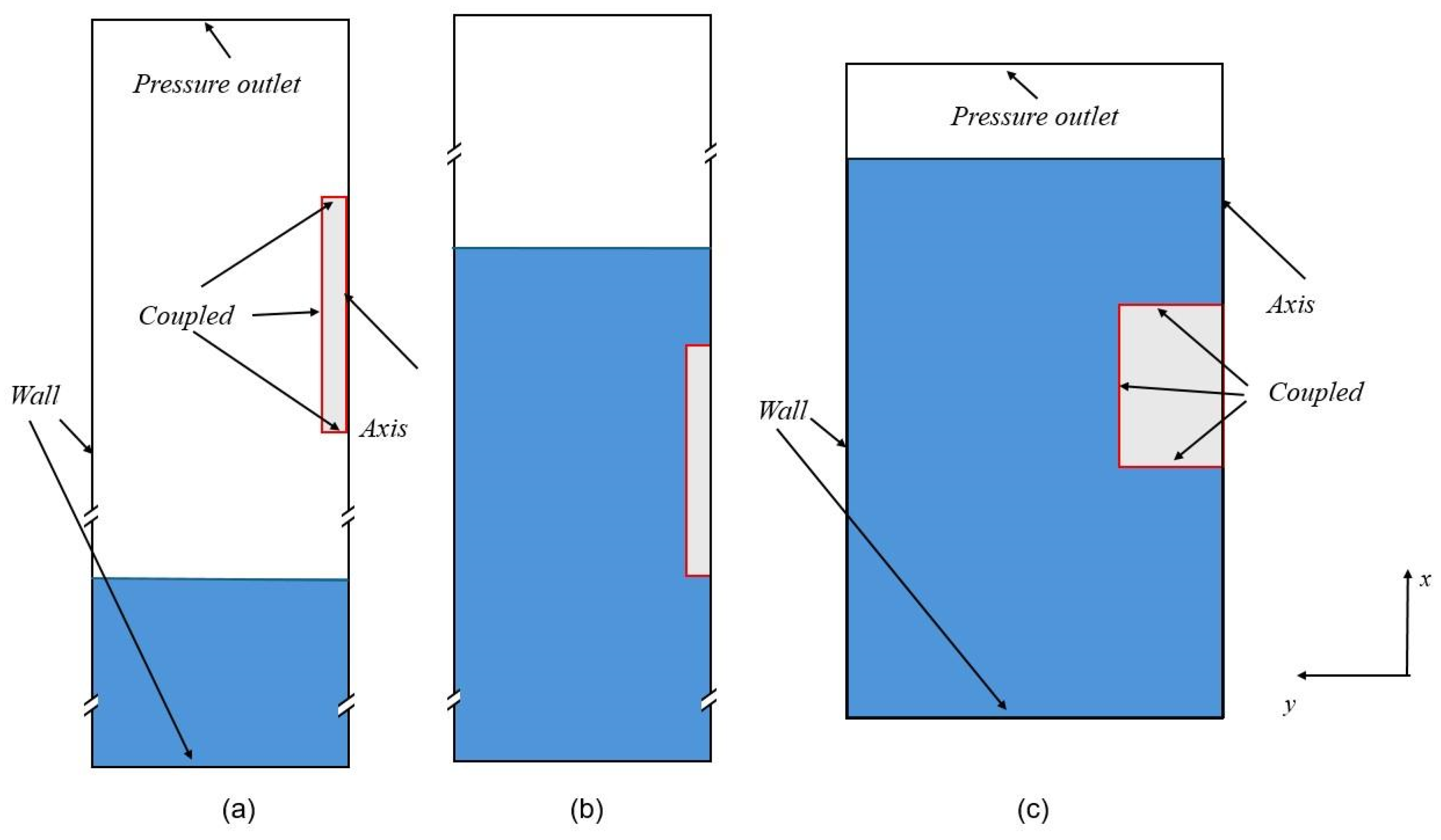
2.2.1. Description of the Cases
2.2.2. General Remarks
2.2.3. Mathematical Model
- conservation of mass:
- conservation of momentum:
- conservation of energy:
2.2.4. Boundary Conditions
2.2.5. Mass Transfer Modeling
2.2.6. Turbulence Modeling
2.2.7. Mesh Motion
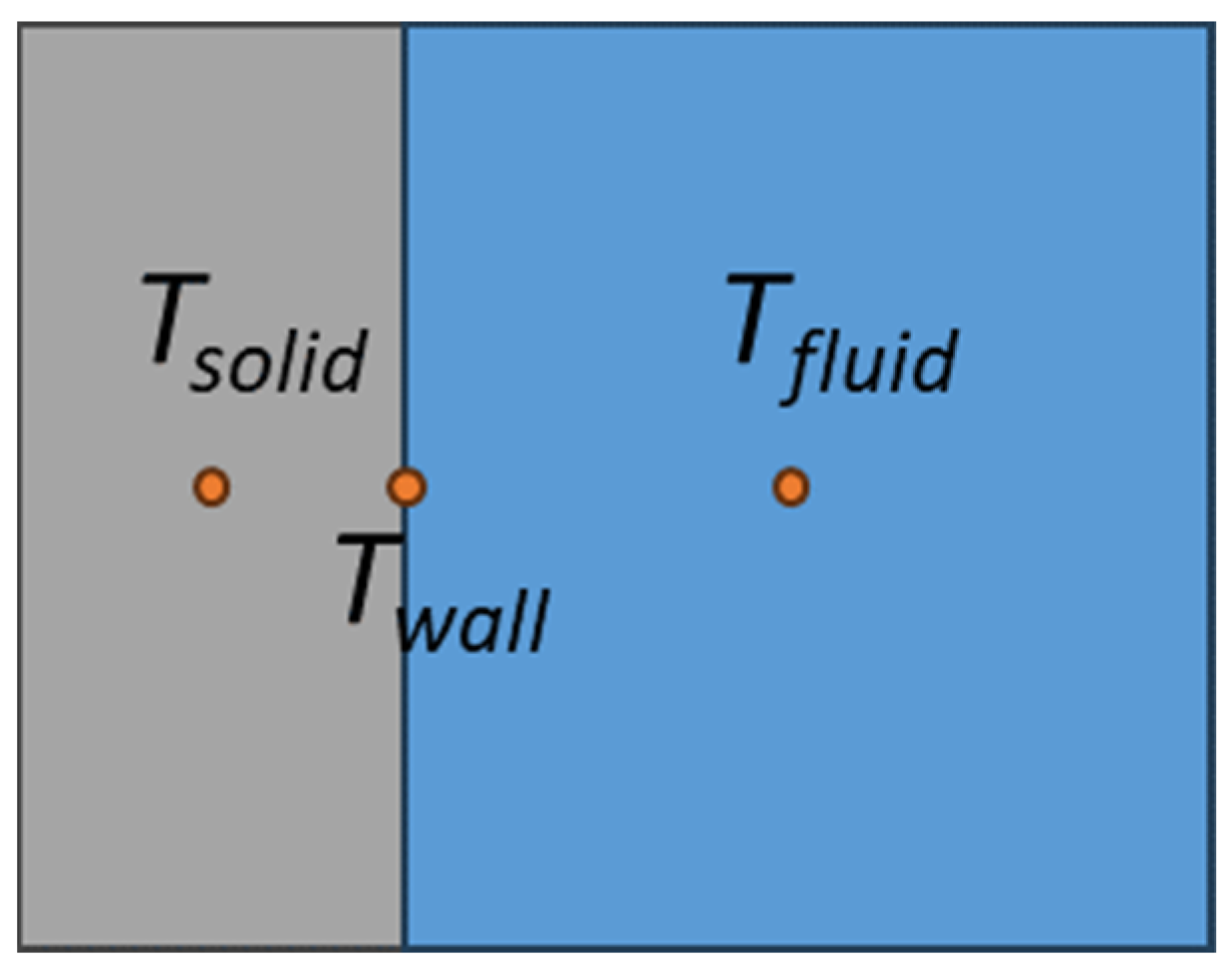
2.2.8. Integral Quantities Calculation: Heat Fluxes and Heat Transfer Coefficients
2.3. Studied Materials
2.3.1. Silver
2.3.2. Inconel 600
3. Results
3.1. Silver Specimen
3.2. Inconel 600 Specimen
4. Conclusions
- Using the already available features of the anisotropic drag model and the zero-resistance and thermal phase change model, a novel mass transfer model has been successfully included within the ANSYS Fluent computational package. The model is included in software via the user-defined functions (UDFs), and the main idea behind model implementation is summarized in the Appendix A.
- The novel method improves the simulations by making it possible to conduct complex boiling computations on a real geometry with real physical properties using moderate computational resources. Furthermore, the empiricism that was associated with the two-fluid model is alleviated by using the two-fluid VOF model in conjunction with the novel mass transfer model and the appropriate closures already available within the ANSYS Fluent.
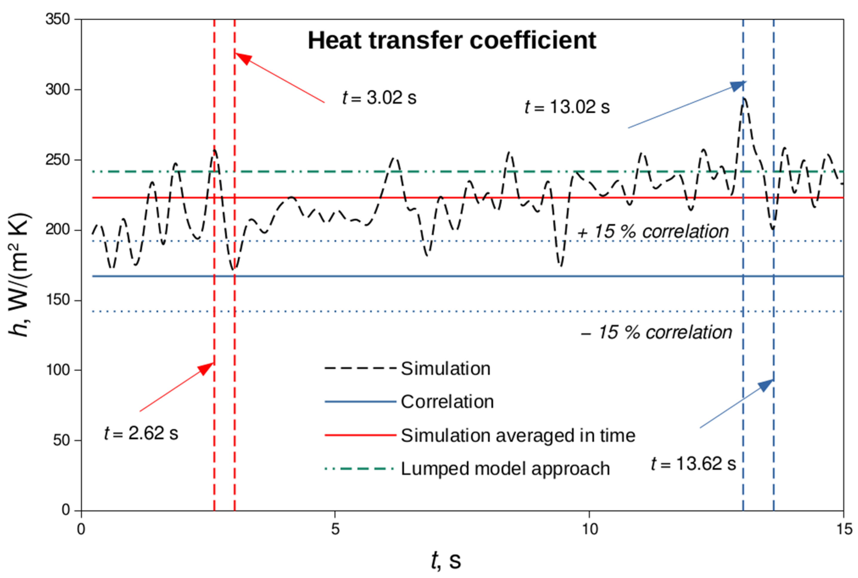
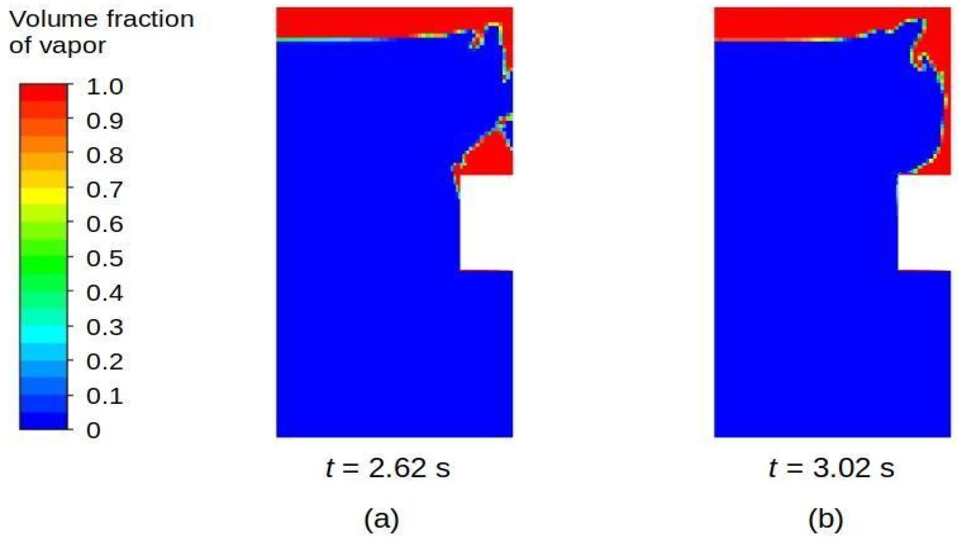
- It was found, at the beginning of the film boiling process, that the bubble collapse yields a peak in the heat transfer coefficient, while the dry zone leads to the local minimum of the heat transfer coefficient (global minimum).
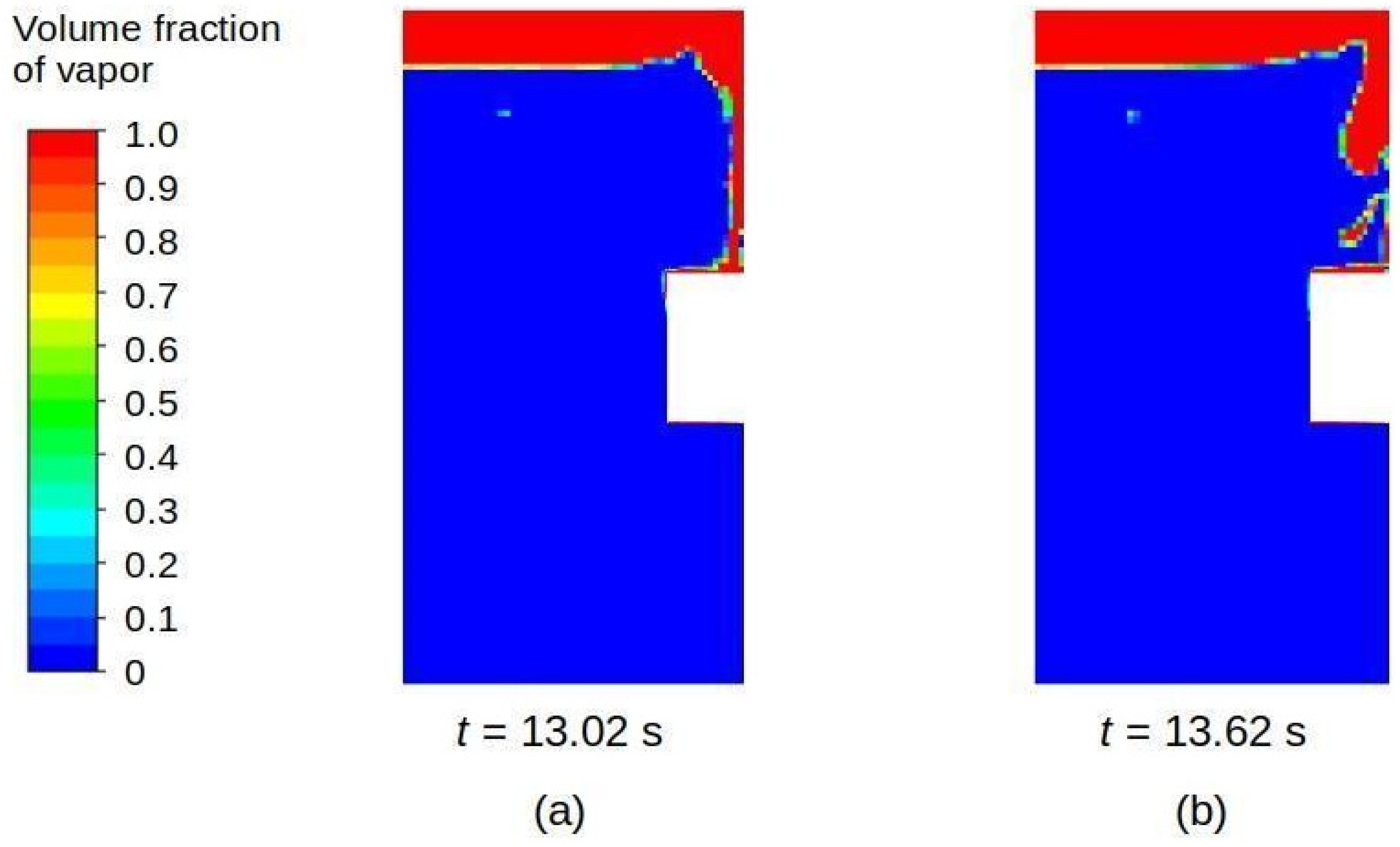
- However, it was not clear at a later stage whether the same finding noted for the second item could be applied, and additional effort is needed in this regard to distinguish the reason for the global maximum and the following local minimum in the heat transfer coefficient.
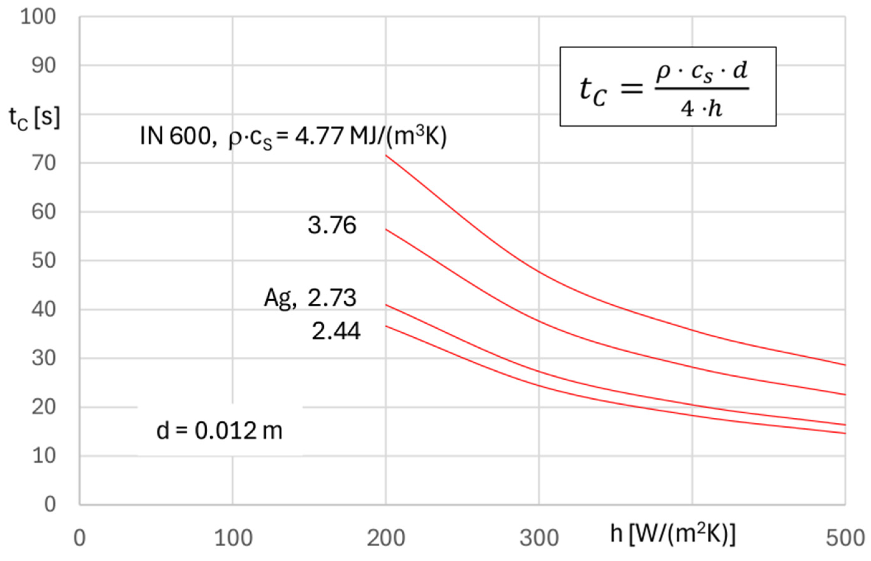
- The proposed lumped heat conduction model that stems from basic principles, i.e., by equalization of the first law of thermodynamics and Newton’s cooling law, was found to be an efficient tool in the estimation of the heat transfer coefficient when the unsteady temperature distribution is known and the time constant could be determined.
Author Contributions
Funding
Institutional Review Board Statement
Informed Consent Statement
Data Availability Statement
Acknowledgments
Conflicts of Interest
Nomenclature
| Latin symbols | ||
| Quantity | Description | Unit |
| Ai | interfacial area density/concentration | m−1 |
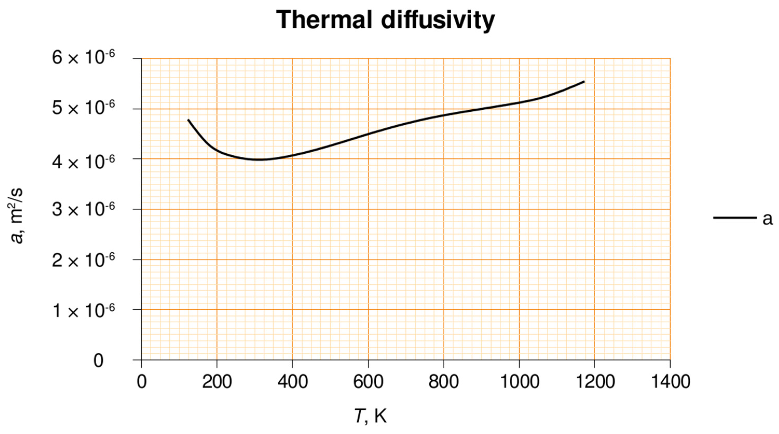
| as | the thermal diffusivity of the solid | m2/s |
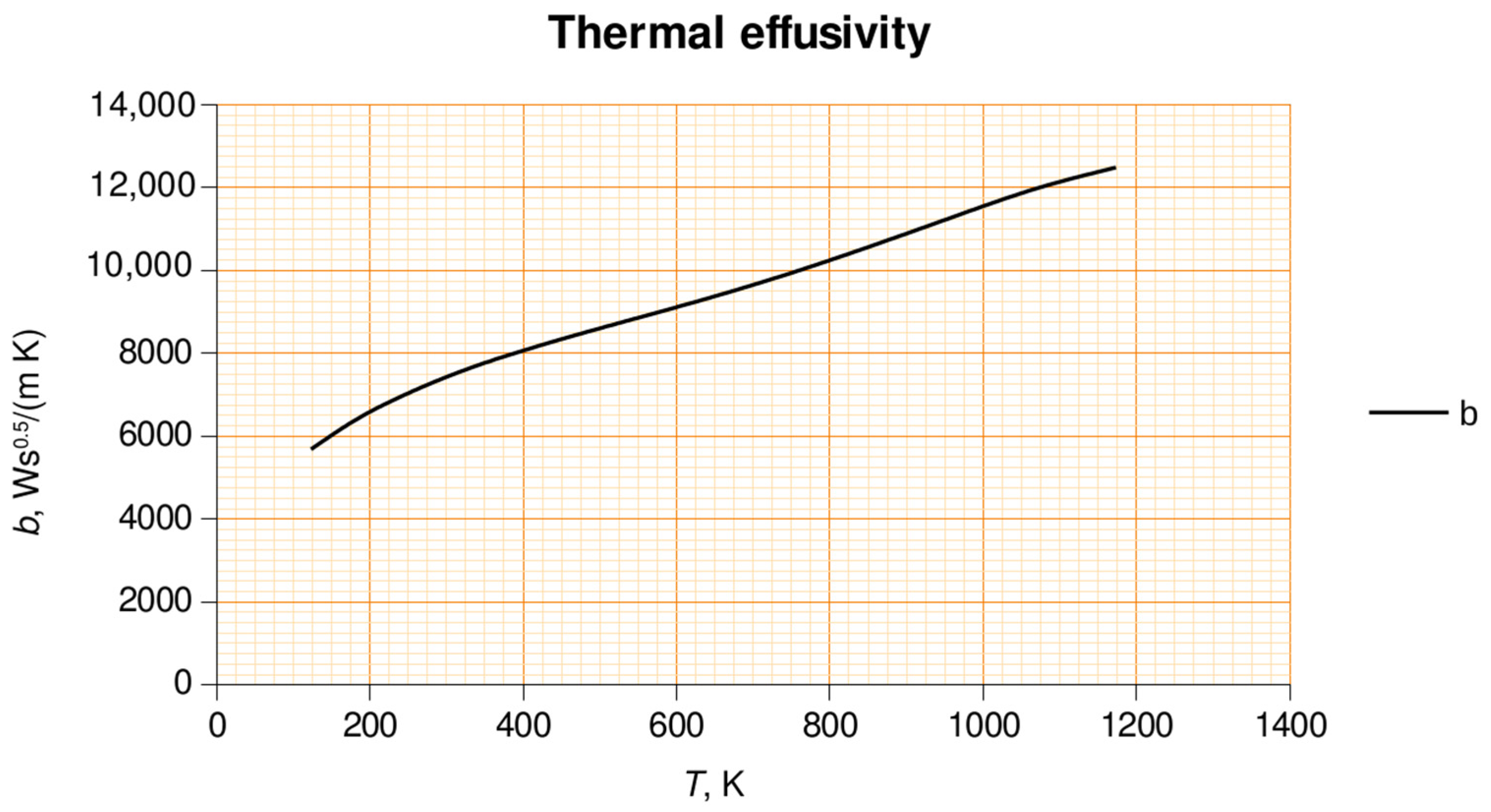
| b | thermal effusivity | Ws0.5/(m K) |
| cs | the specific heat capacity of a solid | J/(kg K) |
| Cv | vapor phase’s scaling factor in the thermal phase change model | 1 |
| D | the diameter | m |
| dv | the vapor phase’s diameter | m |
| g | gravitational acceleration | m/s2 |
| ∇α | gradient of the volume fraction field | m−1 |
| h | the heat transfer coefficient | W/(m2 K) |
| hpq | interphase heat transfer coefficient | W/(m2 K) |
| H | height of a specimen | m |
| mass transfer rate per unit volume for a phase pair | kg/(s m3) | |
| normal vector | m | |
| p | system pressure | Pa |
| ql | heat flux from liquid to the interface | W/m2 |
| qs | heat flux at the solid wall | W/m2 |
| qv | heat flux from vapor phase to the interface | W/m2 |
| r0 | specific heat of vaporization | J/kg |
| general representative of the interface drag term | kg/(m2 s2) | |
| Se | heat flux at the interface (source term) | W/m2 |
| T | thermodynamic (absolute) temperature in degrees Kelvin | K |
| t | time | s |
| Tsat | saturation temperature | K |
| Tsilid | solid temperature | K |
| T∞ | the free stream temperature | K |
| TKE | turbulent kinetic energy (specific) | m2/s2 |
| Tl | liquid phase’s temperature | K |
| Tv | the temperature of the vapor phase | K |
| Tw, Twall | the wall temperature | K |
| up | p-th phase velocity | m/s |
| Vc | cell volume | m3 |
| Vc,i | the volume of i-th cell | m3 |
| the velocity of the phase q (either vapor or liquid) | m/s | |
| w | flow velocity | m/s |
| x | spatial coordinate | m |
| Greek letters | ||
| Quantity | Description | Unit |
| αl | the volume fraction of a liquid phase | 1 |
| αv | the vapor volume fraction | 1 |
| λ | molecular thermal conductivity of a material | W/(m K) |
| λeff | effective thermal conductivity | W/(m K) |
| λm | average thermal conductivity of a solid material | W/(m K) |
| λs | thermal conductivity of a solid material | W/(m K) |
| λt | turbulent thermal conductivity | W/(m K) |
| λvap | thermal conductivity of a vapor phase | W/(m K) |
| μv | the dynamic viscosity of a vapor phase | Pa s |
| νv | the kinematic viscosity of a vapor phase | m2/s |
| ρ | density | kg/m3 |
| ρs | the density of the solid | kg/m3 |
| ρq | density of q-th phase | kg/m3 |
| σ | surface tension | N/m |
| Φpq | the heat flow rate from the interface to the liquid phase in a vapor–liquid phase change process | W/m3 |
Appendix A
References
- Barthès, M. Ebullition Sur Site Isolé: Étude Expérimentale de la Dynamique de Croissance d’une Bulle et des Transferts Associés. Ph.D. Thesis, Université de Provence—Aix-Marseille I, Marseille, France, 2005. [Google Scholar]
- ISO 9950:1995; Industrial Quenching Oils—Determination of Cooling Characteristics—Nickel-Alloy Probe Test Method. International Organization for Standardization: Geneva, Switzerland, 1995.
- Felde, I. Új Módszer Acélok Edzéséhez Használatos Hűtőközegek Hűtőképességének Minősítésére. Ph.D. Thesis, Miskolci Egyetem, Műszaki Anyagtudományi Kar, Kerpely Antal Anyagtudományok és technológiák Doktori Iskola, Miskolc, Hungary, 2007. [Google Scholar]
- Momoki, S.; Yamada, T.; Shigechi, T.; Kanemaru, K.; Yamaguchi, T. Film Boiling Around a Vertical Cylinder With Top and Bottom Horizontal Surfaces. In Proceedings of the HT2007; ASME/JSME 2007 Thermal Engineering Heat Transfer Summer Conference, Vancouver, BC, Canada, 8 July 2007; Volume 2, pp. 611–619. [Google Scholar]
- Demirel, C. Experimentelle Untersuchung und Simulation des Abschreckprozesses von bauteilähnlichen Geometrien aus G-AlSi7Mg. 2009. Available online: https://depositonce.tu-berlin.de/items/a928e92c-4afe-4351-9012-e3b9ad23666b (accessed on 19 November 2024).
- Donnelly, B.; O’Donovan, T.S.; Murray, D.B. Bubble Enhanced Heat Transfer from a Vertical Heated Surface. J. Enhanc. Heat Transf. 2008, 15, 159–169. [Google Scholar] [CrossRef]
- Krause, F.; Schüttenberg, S.; Fritsching, U. Modelling and Simulation of Flow Boiling Heat Transfer. Int. J. Numer. Methods Heat Fluid Flow 2010, 20, 312–331. [Google Scholar] [CrossRef]
- El Kosseifi, N. Numerical Simulation of Boiling for Industrial Quenching Processes; Ecole Nationale Supérieure des Mines de Paris: Paris, France, 2012. [Google Scholar]
- John, V.; Kindl, A.; Suciu, C. Finite Element LES and VMS Methods on Tetrahedral Meshes. J. Comput. Appl. Math. 2010, 233, 3095–3102. [Google Scholar] [CrossRef]
- Magnini, M. CFD Modeling of Two-Phase Boiling Flows in the Slug Flow Regime with an Interface Capturing Technique. Ph.D. Thesis, Alma Mater Studiorum—Università di Bologna, Bologna, Italy, 2012. [Google Scholar]
- Landek, D.; Župan, J.; Filetin, T. A Prediction of Quenching Parameters Using Inverse Analysis. Matls. Perf. Charact. 2014, 3, 229–241. [Google Scholar] [CrossRef]
- Tensi, H.M. Wetting Kinematics. In Theory and Technology of Quenching: A Handbook; Liščić, B., Tensi, H.M., Luty, W., Eds.; Springer: Berlin/Heidelberg, Germany, 1992; pp. 93–116. ISBN 978-3-662-01596-4. [Google Scholar]
- Felde, I.; Shi, W. Hybrid Approach for Solution of Inverse Heat Conduction Problems. In Proceedings of the 2014 IEEE International Conference on Systems, Man, and Cybernetics (SMC), San Diego, CA, USA, 5–8 October 2014; IEEE: Piscataway, NJ, USA, 2014; pp. 3896–3899. [Google Scholar]
- Steuer, R. Ultraschallunterstütztes Flüssigkeitsabschrecken Bei Der Wärmebehandlung Metallischer Werkstoffe; Forschungsberichte des Lehrstuhls für Werkstofftechnik der Universität Rostock; Shaker Verlag: Aachen, Germany, 2015; Volume 4, ISBN 978-3-8440-3667-1. [Google Scholar]
- Subhash, M. Computational Modelling of Liquid Jet Impingement onto Heated Surface. Ph.D. Thesis, Technische Universität: Darmstadt, Darmstadt, Germany, 2017. [Google Scholar]
- Bahbah, C. Méthodes Numériques Avancées Pour La Simulation Du Procédé de Trempe Industrielle. Ph.D. Thesis, Université Paris Sciences et Lettres, Paris, France, 2020. [Google Scholar]
- Panda, A. Direct Numerical Simulations of Heat and Mass Transport in Multiphase Flows. Ph.D. Thesis, Technische Universiteit Eindhoven, Eindhoven, The Netherlands, 2020. [Google Scholar]
- Ebrahim, S.A.; Cheung, F.-B.; Bajorek, S.M.; Tien, K.; Hoxie, C.L. Heat Transfer Correlation for Film Boiling during Quenching of Micro-Structured Surfaces. Nucl. Eng. Des. 2022, 398, 111943. [Google Scholar] [CrossRef]
- Gamidi, K.; Pasam, V.K. Analysis of Residual Stresses in Spot Cooled Vibration Assisted Turning of Ti6Al4V Alloy Using Computational Fluid Dynamics-Aided Finite Element Method. J. Mater. Eng. Perform. 2024, 33, 3731–3745. [Google Scholar] [CrossRef]
- Gupta, P.K.; Yadav, N.P. Numerical Investigation Into Convective Heat Transfer Coefficient of the Grinding Fluid Used in a Deep Grinding Process. Trans. FAMENA 2024, 48, 129–144. [Google Scholar] [CrossRef]
- Hannoschöck, N. Wärmeleitung und -transport: Grundlagen der Wärme- und Stoffübertragung; Springer Berlin Heidelberg: Berlin/Heidelberg, Germany, 2018; ISBN 978-3-662-57571-0. [Google Scholar]
- Bourouga, B.; Gilles, J. Roles of heat transfer modes on transient cooling by quenching process. Int. J. Mater Form 2009, 3, 77–88. [Google Scholar] [CrossRef]
- Cukrov, A.; Sato, Y.; Boras, I.; Ničeno, B. A Solution to Stefan Problem Using Eulerian Two-Fluid VOF Model. Brodogr. Int. J. Nav. Archit. Ocean. Eng. Res. Dev. 2021, 72, 141–164. [Google Scholar] [CrossRef]
- Cukrov, A.; Landek, D.; Sato, Y.; Boras, I.; Ničeno, B. Numerical simulation of film boiling heat transfer in immersion quenching process using Eulerian two-fluid approach. Case Stud. Therm. Eng. 2024, 64, 105497. [Google Scholar] [CrossRef]
- Gauss, F.; Lucas, D.; Krepper, E. Grid Studies for the Simulation of Resolved Structures in an Eulerian Two-Fluid Framework. Nucl. Eng. Des. 2016, 305, 371–377. [Google Scholar] [CrossRef]
- Liu, Y.; Pointer, W.D. Eulerian Two-Fluid RANS-Based CFD Simulations of a Helical Coil Steam Generator Boiling Tube; Oak Ridge National Lab. (ORNL): Oak Ridge, TN, USA, 2017. [Google Scholar]
- Ansys® Fluent. ANSYS Fluent Theory Guide, Release 19.2; Help System; ANSYS, Inc.: Canonsburg, PA, USA, 2019. [Google Scholar]
- Perić, M. Modeling of Free-Surface Flow With Focus on the VOF-Method. In Proceedings of the 17th Multiphase Flow Conference and Short Course, Helmholtz-Zentrum Dresden—Rossendorf, Dresden, Germany, 11–15 November 2019. [Google Scholar]
- Drew, D.A.; Passman, S.L. Theory of Multicomponent Fluids; Springer Science & Business Media: Berlin/Heidelberg, Germany, 2006; Volume 135, ISBN 0-387-22637-0. [Google Scholar]
- Höhne, T.; Vallée, C. Experiments and Numerical Simulations of Horizontal Two-Phase Flow Regimes Using an Interfacial Area Density Model. J. Comput. Multiph. Flows 2010, 2, 131–143. [Google Scholar] [CrossRef]
- Denèfle, R.; Mimouni, S.; Caltagirone, J.-P.; Vincent, S. Multifield Hybrid Approach for Two-Phase Flow Modeling—Part 1: Adiabatic Flows. Comput. Fluids 2015, 113, 106–111. [Google Scholar] [CrossRef]
- Kharangate, C.R.; Lee, H.; Mudawar, I. Computational Modeling of Turbulent Evaporating Falling Films. Int. J. Heat Mass Transf. 2015, 81, 52–62. [Google Scholar] [CrossRef]
- Mer, S.; Praud, O.; Neau, H.; Merigoux, N.; Magnaudet, J.; Roig, V. The Emptying of a Bottle as a Test Case for Assessing Interfacial Momentum Exchange Models for Euler–Euler Simulations of Multi-Scale Gas-Liquid Flows. Int. J. Multiph. Flow 2018, 106, 109–124. [Google Scholar] [CrossRef]
- Štrubelj, L.; Tiselj, I.; Mavko, B. Simulations of Free Surface Flows with Implementation of Surface Tension and Interface Sharpening in the Two-Fluid Model. Int. J. Heat Fluid Flow 2009, 30, 741–750. [Google Scholar] [CrossRef]
- de Bertodano, M.L.; Fullmer, W.; Clausse, A.; Ransom, V.H. Introduction. In Two-Fluid Model Stability, Simulation and Chaos; de Bertodano, M.L., Fullmer, W., Clausse, A., Ransom, V.H., Eds.; Springer International Publishing: Cham, Switzerland, 2017; pp. 1–8. ISBN 978-3-319-44968-5. [Google Scholar]
- Malikov, Z. Mathematical Model of Turbulence Based on the Dynamics of Two Fluids. Appl. Math. Model. 2020, 82, 409–436. [Google Scholar] [CrossRef]
- Kharangate, C.R.; Mudawar, I. Review of Computational Studies on Boiling and Condensation. Int. J. Heat Mass Transf. 2017, 108, 1164–1196. [Google Scholar] [CrossRef]
- Cukrov, A.; Sato, Y.; Boras, I.; Ničeno, B. Film Boiling around a Finite Size Cylindrical Specimen—A Transient Conjugate Heat Transfer Approach. Appl. Sci. 2023, 13, 9144. [Google Scholar] [CrossRef]
- Hillier, A.; Doorsselaere, T.V.; Karampelas, K. Estimating the Energy Dissipation from Kelvin–Helmholtz Instability Induced Turbulence in Oscillating Coronal Loops. ApJL 2020, 897, L13. [Google Scholar] [CrossRef]
- Yamada, T.; Shigechi, T.; Momoki, S.; Kanemaru, K. An Analysis of Film Boiling around a Vertical Finite-Length Cylinder. Rep. Fac. Eng. Nagasaki Univ. 2001, 31, 1–11. [Google Scholar]
- Aubram, D. An Arbitrary Lagrangian-Eulerian Method for Penetration into Sand at Finite Deformation; Shaker: Düren, Germany, 2014; ISBN 978-3-8440-2507-1. [Google Scholar]
- Cukrov, A.; Landek, D.; Sato, Y.; Boras, I.; Ničeno, B. Water Entry of a Heated Axisymmetric Vertical Cylinder. Energies 2023, 16, 7926. [Google Scholar] [CrossRef]
- Dobrzynski, C. Adaptation de Maillage Anisotrope 3D et Application à l’aéro-Thermique Des bâtiments. Ph.D. Thesis, Université Pierre et Marie Curie—Paris VI, Paris, France, 2005. [Google Scholar]
- Olivier, G. Anisotropic Metric-Based Mesh Adaptation for Unsteady CFD Simulations Involving Moving Geometries, Adaptation de Maillage Anisotrope Par Prescription de Champ de Métriques Appliquée Aux Simulations Instationnaires En Géométrie Mobile; Université Pierre et Marie Curie—Paris VI: Paris, France, 2011. [Google Scholar]
- Barral, N. Time-Accurate Anisotropic Mesh Adaptation for Three-Dimensional Moving Mesh Problems, Adaptation de Maillage Anisotrope Dépendant Du Temps Pour Des Problèmes Tridimensionnels En Maillage Mobile; Université Pierre et Marie Curie—Paris VI: Paris, France, 2015. [Google Scholar]
- MacKenzie, D.S. Understanding the Cooling Curve Test. Therm. Process. 2017, 28–32. Available online: https://thermalprocessing.com/wp-content/uploads/2017/201701/0117-ASM.pdf (accessed on 19 November 2024).
- Jagga, S.; Vanapalli, S. Cool-down Time of a Polypropylene Vial Quenched in Liquid Nitrogen. Int. Commun. Heat Mass Transf. 2020, 118, 104821. [Google Scholar] [CrossRef]
- Mayinger, F. Blasenbildung und Wärmeübergang beim Sieden in freier und erzwungener Konvektion. Chem. Ing. Tech. 1975, 47, 737–748. [Google Scholar] [CrossRef]
- Bucci, M.; Buongiorno, J.; Bucci, M. The Not-so-Subtle Flaws of the Force Balance Approach to Predict the Departure of Bubbles in Boiling Heat Transfer. Phys. Fluids 2021, 33, 017110. [Google Scholar] [CrossRef]
- Cukrov, A.; Landek, D.; Sato, Y.; Boras, I.; Ničeno, B. The Development of Numerical Method for Simulation of Metal Materials Quenching. Rud. Geol. Naft. Zb. 2025, 40. in press. [Google Scholar]
- Sato, Y.; Ničeno, B. Pool boiling simulation using an interface tracking method: From nucleate boiling to film boiling regime through critical heat flux. Int. J. Heat Mass Transf. 2018, 125, 876–890. [Google Scholar] [CrossRef]
Disclaimer/Publisher’s Note: The statements, opinions and data contained in all publications are solely those of the individual author(s) and contributor(s) and not of MDPI and/or the editor(s). MDPI and/or the editor(s) disclaim responsibility for any injury to people or property resulting from any ideas, methods, instructions or products referred to in the content. |
© 2025 by the authors. Licensee MDPI, Basel, Switzerland. This article is an open access article distributed under the terms and conditions of the Creative Commons Attribution (CC BY) license (https://creativecommons.org/licenses/by/4.0/).
Share and Cite
Cukrov, A.; Sato, Y.; Landek, D.; Hannoschöck, N.; Boras, I.; Ničeno, B. Determination of Heat Transfer Coefficient in a Film Boiling Phase of an Immersion Quenching Process. Appl. Sci. 2025, 15, 1021. https://doi.org/10.3390/app15031021
Cukrov A, Sato Y, Landek D, Hannoschöck N, Boras I, Ničeno B. Determination of Heat Transfer Coefficient in a Film Boiling Phase of an Immersion Quenching Process. Applied Sciences. 2025; 15(3):1021. https://doi.org/10.3390/app15031021
Chicago/Turabian StyleCukrov, Alen, Yohei Sato, Darko Landek, Nikolaus Hannoschöck, Ivanka Boras, and Bojan Ničeno. 2025. "Determination of Heat Transfer Coefficient in a Film Boiling Phase of an Immersion Quenching Process" Applied Sciences 15, no. 3: 1021. https://doi.org/10.3390/app15031021
APA StyleCukrov, A., Sato, Y., Landek, D., Hannoschöck, N., Boras, I., & Ničeno, B. (2025). Determination of Heat Transfer Coefficient in a Film Boiling Phase of an Immersion Quenching Process. Applied Sciences, 15(3), 1021. https://doi.org/10.3390/app15031021