Discoloration Characteristics of Mechanochromic Sensors in RGB and HSV Color Spaces and Displacement Prediction

Abstract

Mechanochromic sensors are promising for structural health monitoring as they can visually monitor the deformation caused by discoloration. Most studies have focused on the large deformation problems over 100% strain; however, it is necessary to investigate the discoloration characteristics in a small deformation range to apply it to engineering structures, such as reinforced concrete. In this study, a photonic crystal-based discoloration sensor was investigated to determine the discoloration characteristics of the red, green, and blue (RGB) as well as hue, saturation, and value (HSV) color spaces according to displacement levels. B and S showed the highest sensitivity and linear discoloration at displacements < 1 mm, whereas R and H showed significant discoloration characteristics at displacements > 1 mm. The Vision Transformer model based on RGB and HSV channels was linearly predictable up to 4 mm displacement with an accuracy of R² 0.89, but errors were found at the initial displacement within 2 mm.

1. Introduction

The real-time monitoring of structures during construction or operation stages is crucial for ensuring structural safety and preventing unforeseen accidents or failures. Current monitoring systems largely utilize electronic devices such as strain and displacement sensors to measure mechanical deformations by applying the concept of electrical resistance changes. Although these technologies can be sophisticated and accurate, they also have limitations such as high initial installation and maintenance costs, low durability, need for technical expertise, and the requirement of placing sensors in hard-to-access locations [1].

To overcome these obstacles, various structural health monitoring (SHM) systems have been introduced as potential diagnostic techniques for engineering structures. For example, acoustic emissions can effectively detect the development of a crack and its position in advance. However, the frequency components of acoustic emission signals are not always reliable indicators of material damage, as they can be affected by the wave propagation distance [2], making it difficult to interpret the signals. Fiber-optic sensors offer many advantages, such as low power loss, immunity to electromagnetic interference, compact size, and durability in harsh environments for SHM diagnosis systems; however, several challenges remain, including difficulties in interpreting signals (high noise and sensitivity for low-amplitude signals) [3] and complex wiring systems [4].

Mechanochromic substances, which change color in response to mechanical deformations, offer opportunities in the construction industry [5]. These substances can be attached to the components that make up the structure, and their discoloration provide an intuitive, immediate visual cue of potential failures [6,7], enabling real-time, at-a-glance diagnostics. They can be applied as a part of the attachment process during or after the construction phase, thereby significantly simplifying the installation process and reducing the need for specialized equipment and technical expertise. Furthermore, because they do not rely on data transmission, they allow for immediate response and intervention. Additionally, the monitoring systems require minimal maintenance as they do not require power or electronic components to function, further reducing long-term operational costs. Therefore, such mechanochromic substances are particularly advantageous in the diagnosis systems of large-scale structures requiring real-time data transmission and present as a promising sensor for SHM [8,9,10].

Minh et al. [5] fabricated a photonic crystal (PC) mechanochromic sensor by assembling polystyrene nanoparticles on a silicon wafer via spin coating. They discovered discoloration of the sensor from blue to red when it was stretched by 50%. The diffracted wavelength increased linearly from 450 to 670 nm when strain from 0 to 50% was applied, indicating a high degree of sensitivity in this strain range. Zhang et al. [11] employed a nanoimprinting technique to fabricate polystyrene nanoparticles based on a PC mechanochromic sensor. The discoloration of the sensor could be distinguished at strains below 30%, and it maintained its mechanochromic ability after 2000 cycles of a stretching test. Bae et al. [7] developed a Fabry–Pérot (F-P) mechanochromic sensor composed of metal–insulator–metal cavity structures. This sensor can be stretched over 100%, i.e., it can be deformed beyond the initial length before deformation. Also, this sensor displays distinct angle-insensitive color changes in response to mechanical strain (percentage of displacement relative to the initial length). Another study by this group [6] proposed a colorimetric method for detecting deformation in Al-based metals using a mechanochromic sensor with a strain capacity (maximum strain) of 120%. This method achieved an error rate of less than 15% compared to the actual strain. Pyeon et al. [12] discovered that the discoloration of an F-P mechanochromic sensor could be detected in real time during crack propagation in fiber-reinforced concrete. Furthermore, the discoloration ability of the mechanochromic sensor exposed to a freeze–thaw environment was restored in 2 h.

Reinforced concrete is the main composite used in structures in the civil and architectural fields. Steel reinforcements cause critical damages at about 0.02% of strain. As concrete is used as a covering to prevent corrosion of the reinforced steel, cracks in the concrete cover can deteriorate reinforced concrete structures and are required to be strictly managed according to design standards. For instance, the American Concrete Institute [13] and Korean Concrete Institute [14] generally adopt cracks of 0.3 mm as the allowable crack size under humidity conditions to inhibit the corrosion of rebar. Because the crack width of concrete is measured with the naked eye using a crack width ruler, the assessment of crack width may be subject to the worker’s individual judgement.

Previously reported mechanochromic sensors can be deformed to more than 100%, and their discolorations are effective within 50% strain. Therefore, it is important to perform a sensitivity analysis of the mechanochromic sensor discoloration for its application in SHM. In this study, the discoloration sensitivity of the mechanochromic sensor was analyzed to investigate its feasibility as a mechanical sensor for SHM in the construction field. Therefore, since the crack width of concrete is managed in terms of length rather than strain, displacement was chosen as the measure of deformation. Uniaxial direct tensile tests were conducted on a steel plate with a mechanochromic sensor attached. The discoloration of the mechanochromic sensor was quantified in the red, green, and blue (RGB) as well as hue, saturation, and value (HSV) color spaces using image analysis and compared with the real displacement. Additionally, we propose a method for regressing displacement by simultaneously inputting each color space into the deep learning algorithm, enabling feature extraction from each color space and integrating the entire displacement process of the mechanochromic sensor into one process.

2. Preparation and Methodology

2.1. Fabrication of Mechanochromic Sensor

The fabrication process for the mechanochromic sensor is illustrated in Figure 1. A 780 nm monolayer of polystyrene particles (Bangs Laboratories, Inc., Fishers, IN, USA) was assembled using a spin-coating method, as previously reported [15]. Subsequently, it was etched in an oxygen-reactive ion chamber (RIE) to reduce its mean diameter. A 200 nm (Cr) film was then deposited on the substrate using an e-beam evaporator. After peeling off the nanoparticles using adhesive tape, a master mold with concave nanostructures was obtained for further replication on a polydimethylsiloxane (PDMS) substrate. In this study, a PDMS substrate with convex nanostructures (nanobumps) on its surface served as a mechanochromic sensor.

Since the color on the sensor is generated by the interaction between the incident light and the periodic nanobumps, its color is determined by the periodicity of the nanobumps if the angle of incident light is fixed. When the sensor is stretched to certain strain ($\mathsf{\epsilon }$), the initial lattice constant (${\mathrm{d}}_0$) shifts to ${\mathrm{d}}^{\prime }={\mathrm{d}}_0(1+\mathsf{\epsilon })$ [16]. The diffracted wavelength of the undeformed sensor (${\mathsf{\lambda }}_0$) is determined by the incident angle (${\mathsf{\theta }}_1$) and diffracted angle (viewing angle, ${\mathsf{\theta }}_2$). Therefore, the diffracted wavelength shift (${\mathsf{\lambda }}^{\prime }$) due to deformation is given by:

$${\mathsf{\lambda }}^{\prime }={\mathsf{\lambda }}_0(1+\mathsf{\epsilon })$$

(1)

Figure 2 shows the reflection spectra of the sensor as a function of wavelength to depict its color variation for different strain levels. This result was obtained under conditions where the incident angle (${\mathsf{\theta }}_1$) and the viewing angle (${\mathsf{\theta }}_2$) were set to 40° and 0°, respectively. The initial color of the sensor was blue. As the strain increased, the peak of wavelength spectrum shifted to a higher region of wavelength (Figure 2a). At strains of 0%, 10%, 20%, 30%, 40%, and 50%, the sensor displayed blue, light blue, green, yellow, orange, and red colors, respectively. It was noted that the reflection intensity became weaker with increasing the strain. This might be because tensile deformation caused wrinkles on the surface of the sensor [7] and contraction of the nanostructure in height due to the Poisson effect [17].

As indicated in the above equation, the wavelength changed linearly with the strain. The measured wavelengths corresponding to various strain levels were accurately predicted by Equation (1) (gray arrow in Figure 2b).

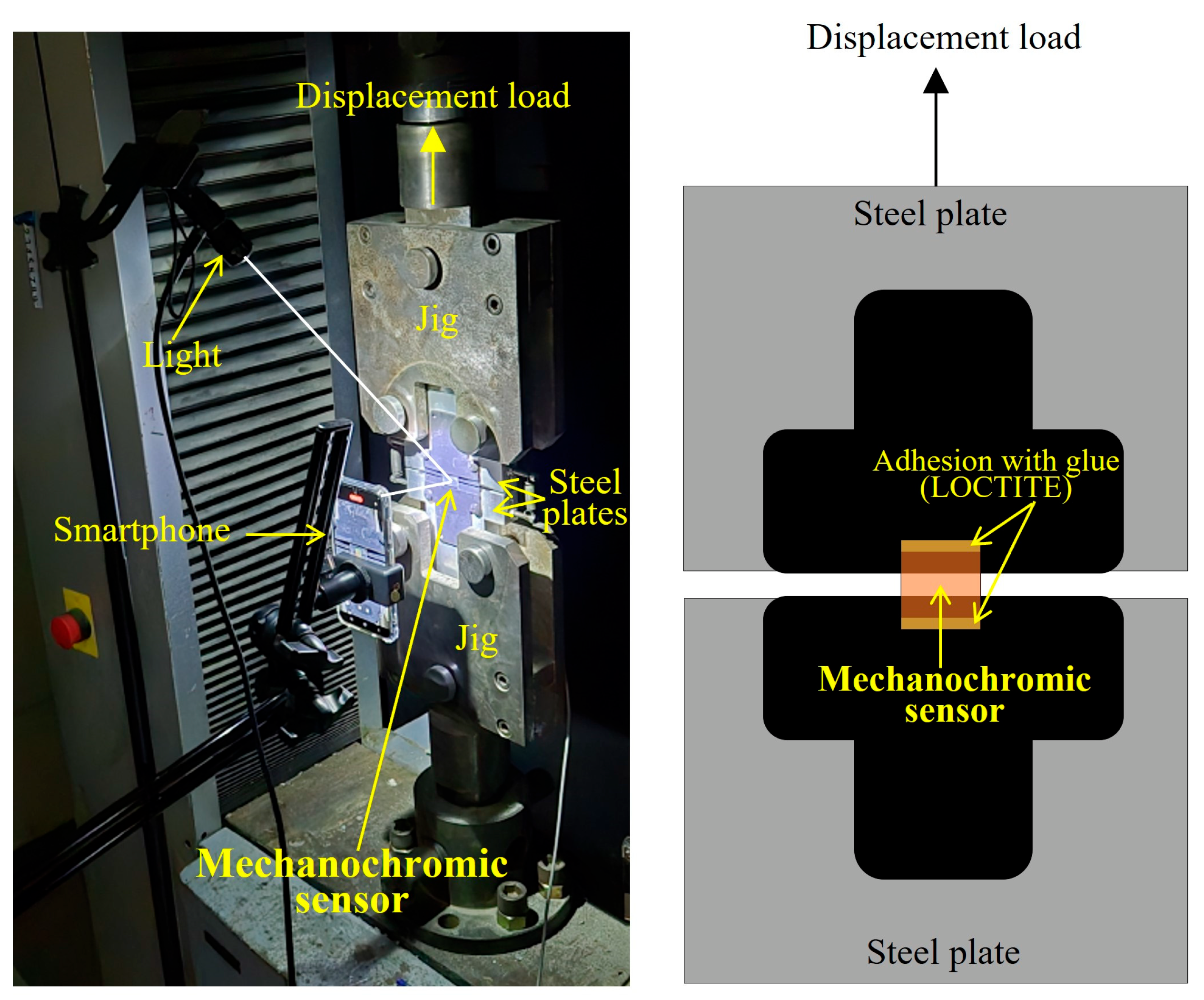
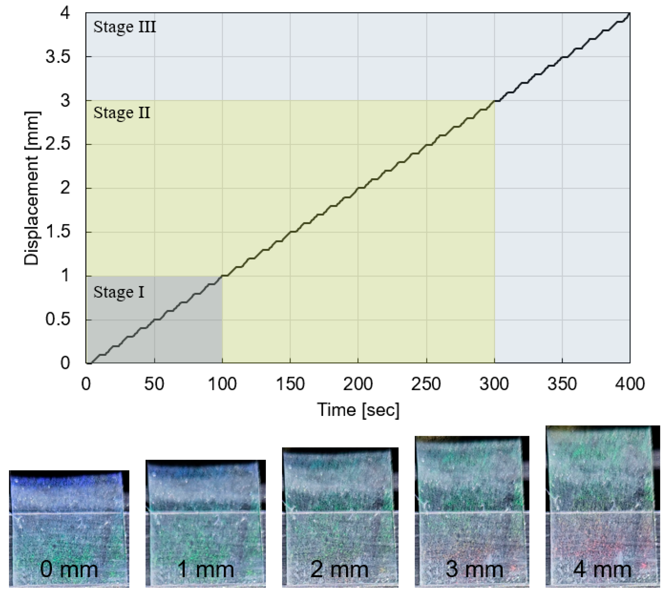
2.2. Measurements of Discoloration and Displacement Under Tensile Load

To induce the deformation of the mechanochromic sensor, a direct tensile test was employed. The tensile test setup is shown in Figure 3. A steel plate was installed on the upper and lower parts of the jig, respectively, and a sensor was attached to the adhesive between them. A uniaxial tensile displacement of up to 4 mm was applied and paused every 0.1 mm. An image of the sensor discoloration according to the displacement is shown in Figure 4. Stroke displacement was recorded using a universal testing machine (AG-300KMX; Shimadzu, Kyoto, Japan). The entire experimental process was recorded using a smartphone (Galaxy s23, Samsung Electronics Inc., Suwon, Republic of Korea). The distance between the camera lens and the sensor was set to 8 cm, and the angle (${\mathsf{\theta }}_2$) of the light reflected from the sensor to the camera lens was set to 0°. An artificial light source was installed to create a constant-illuminance environment at an incident angle (${\mathsf{\theta }}_1$) of 55°. The illuminance from the artificial light source was measured (MK350S; Uprtek, Taiwan, China) three times at the center of the sensor before and after the tensile test, confirming constant illuminance (9847 lx). The discoloration of a mechanochromic sensor, especially a PC-based sensor, has different color development characteristics according to the incident angle of light and the lattice spacing of the nanostructure. However, this study focused on investigating the correlation between the discoloration and deformation of the mechanochromic sensor under photographing conditions, including constant illuminance, capturing distance, and equipment. Discoloration in different environments should be investigated in future studies.

2.3. Methodology of Image Analysis for Quantification of Discoloration

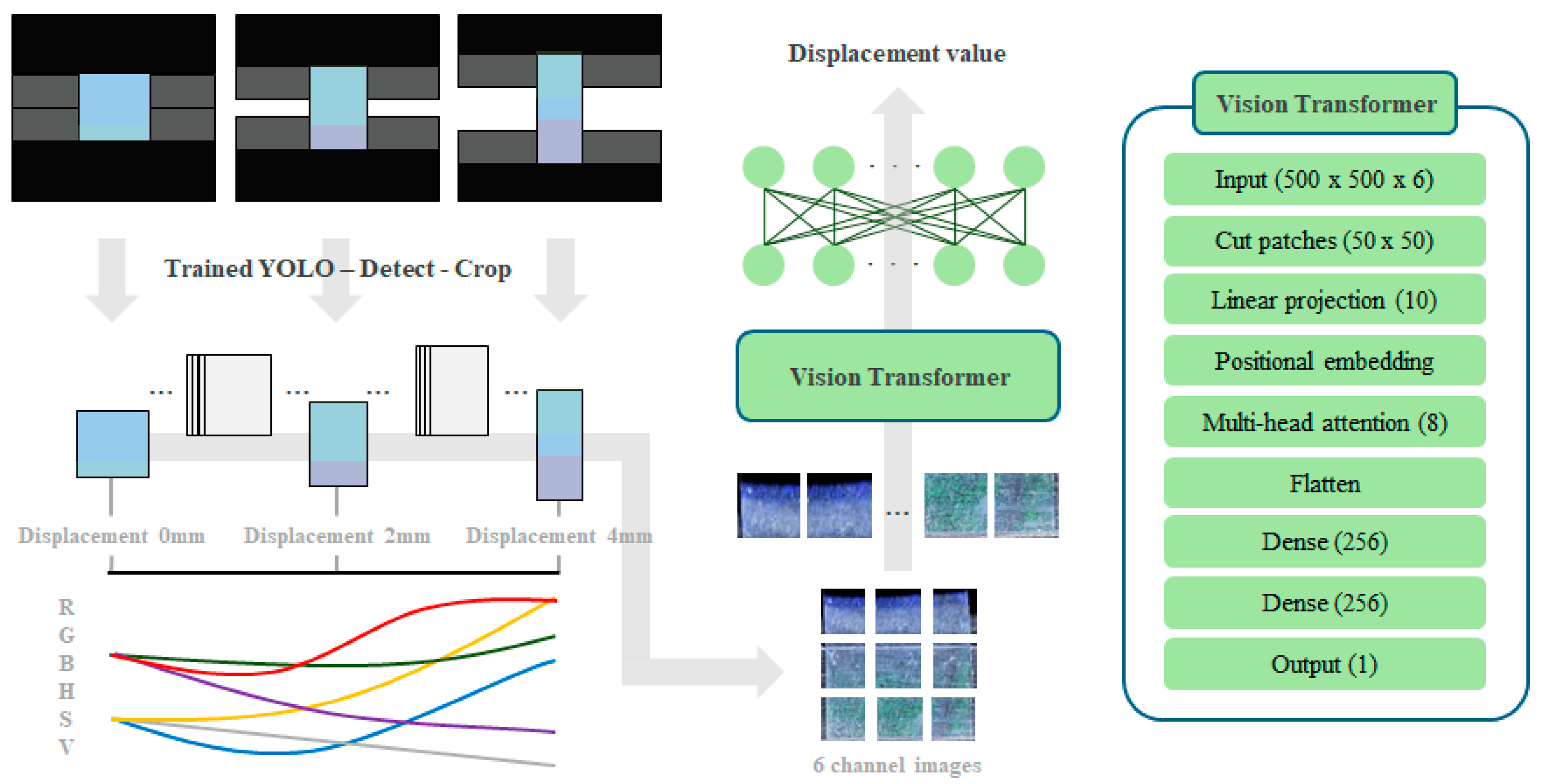
2.3.1. Image Processing

Figure 5 shows the workflow used to quantify the discoloration of the mechanochromic sensor. Colorimetric changes in a displacement-responsive mechanochromic sensor were quantified in both the RGB and HSV color spaces, and the Vision Transformer (ViT) algorithm [18] was used to regress the corresponding displacement values. To convert the sensor region from the raw images into defined objects, polygon-style labels were obtained from 245 sensor images using the LabelMe software (version 5.6.0), open-source image annotation tool, and fine-tuning methods were applied to customize the YOLO v8 model. The trained model detected and cropped sensor regions from raw time-sequence images, which included displacements ranging from 0–3 mm at intervals of 0.1/6 mm/s.

The extracted sensor images were clustered and quantized into 15 colors by using a k-means clustering algorithm. The images were then converted into HSV channels, concatenated with the original RGB channels, and then concatenated into six channel sensor images. The mean intensity of each channel was calculated and matched with displacement values over time. The changes were compared and analyzed in three displacement stages: 0–1 mm, 1–3 mm, and 3–4 mm.

2.3.2. Vision Transformer

ViT uses attention layers to learn the significance of pixels within an image, thereby enabling meaningful inferences from the images. In this study, we employed a Vision Transformer for a small-sized dataset algorithm (ViT-s) [19] that can achieve high-performance regression even with a limited-size dataset.

For input preprocessing, the extracted six channel sensor images were resized to a resolution of 500 × 500 pixels and divided into patches of 50 pixels each. Each patch was flattened and vectorized into a size of 10 using a linear projection layer. The positional information for each patch was added to retain the spatial context of the original image. The vectors were processed through eight transformer layers, followed by a two-layer multilayer perceptron architecture, each comprising 256 perceptrons. Model outputs predicted displacement values.

3. Results and Discussion

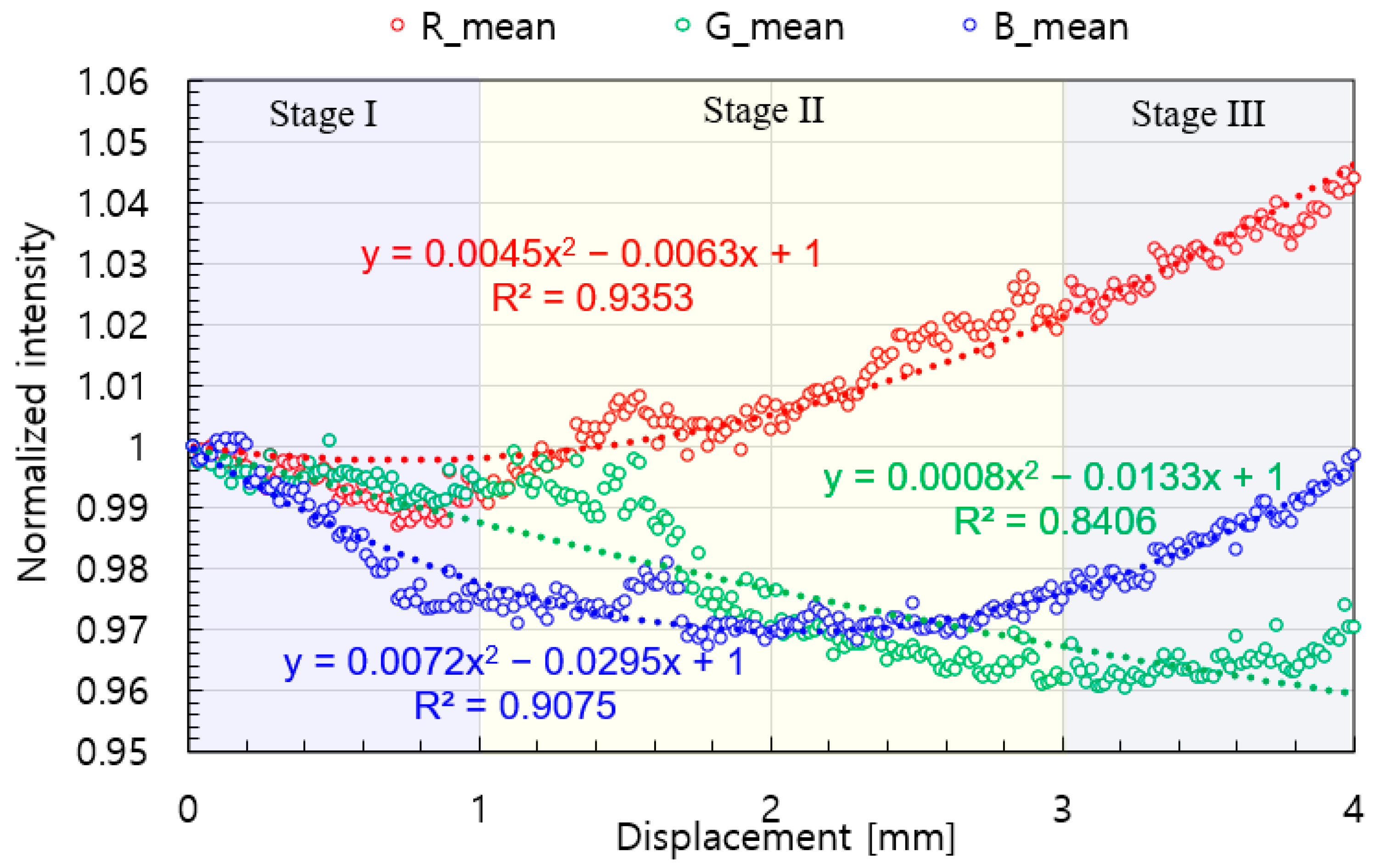
3.1. Relationship Between Deformation and RGB Values

Figure 6 shows the intensities of R, G, and B values with respect to the applied displacement. The R, G, and B values were normalized as the ratios of the intensities changed by deformation to the initial intensities. The changes in R, G, and B values varied depending on the displacement level.

In stage I (0–1 mm), R, G, and B showed discoloration characteristics. The B values were the most sensitive to the initial displacement, showing a relatively steep slope. The R and G values were similar during this stage and showed a slight decrease. R and G showed different behaviors from those at stage II (1–3 mm). R increased continuously until the end of this stage, whereas the G values remained constant up to 1.5 mm, followed by a sharp decrease up to 2 mm. Subsequently, this decrease slowed down. Within this displacement range, the decrease in B slowed, and B increased from 2 mm; however, overall, it showed low-sensitivity discoloration. In stage III (3–4 mm), the R value increased. In contrast, G showed an increasing trend from 3.5 mm, which was similar to the trend observed from 0.8 to 1.5 mm in stage I and II. However, B showed an increasing trend until the end of the experiment at 4 mm and showed a slope similar to that of R. Owing to these characteristics, RGB can be appropriately defined as a polynomial function (dotted lines in Figure 6) within the 0–4 mm displacement range. These relationships are consistent with those reported previously [6]. R and B exhibited R² values of over 0.91 in relation to displacement, while G showed an R² value of 0.84.

Consequently, in the initial displacement of stage I, B showed the dominant discoloration characteristic, whereas G showed the main discoloration in stage II. The discoloration of R showed remarkable discoloration characteristics at displacements of 1 mm or more, including stages II and III; that is, a large displacement. This is owing to the change in the reflection characteristics according to the deformation of the internal structure of the mechanochromic sensor. This trend aligns with the wavelength shift shown in Figure 2, where the color changed sequentially from blue to green to red as the strain increased. Color B, which was sensitive during the initial displacement in stage I, reappeared prominently in stage III due to the periodicity of discoloration governed by Bragg’s diffraction equation ($\mathsf{\lambda }=2\mathrm{d}·\mathrm{s}\mathrm{i}\mathrm{n}\mathsf{\theta })$. This observation is consistent with previous observation [16], which reported that the color of the sensor returned to its initial B beyond a strain of 50% (4 mm displacement). However, the color in this second cycle was deteriorated. Therefore, the discoloration of the sensor in the first cycle is effective for predicting deformation, while the reliability of using discoloration in the second cycle remains questionable.

3.2. Relationship Between Deformation and HSV Values

Figure 7 shows the changes in the intensities of H, S, and V as functions of the applied displacement. HSV is a digital color format in which a specific color is defined by its position coordinates in a cylindrical coordinate, where H is the angle, S is the radius, and V is the height. This allows intuitive color changes, particularly for visualizing sensitive changes in hue and saturation [20]. H, S, and V were normalized to the ratios of the intensities changed by deformation to the initial intensities.

In stage I (0–1 mm), S showed the most sensitive discoloration compared to H and V; that is, a decrease in saturation was clearly observed. The H and V values showed minor decreases, and their behaviors were similar during this stage. The high sensitivity of S in this stage suggests that initial structural deformation induced increased scattering, which lowered the purity of color. Beyond stage I, S still showed a large decrease, and H started to increase significantly beyond 1.5 mm, indicating a shift in the reflected wavelength toward longer (redder) one due to structural elongation. However, no significant change was observed in V in stage II. In stage III, H and S appeared to converge along with a decrease in their slopes, and V still showed no significant change, except for a slight increase toward the end of the experiment. These results suggest that H, S, and V values reflect the periodic deformation of the sensor’s internal structure, governed by Bragg’s diffraction equation, and align with the RGB discoloration trend of B → G → R. Furthermore, the polynomial relationships (each dotted line in Figure 7) between H, S, and V and the applied displacement (with R² > 0.84) highlight the non-linear deformation behavior of the sensor, indicating the influence of nanoscale structural reconfiguration at higher displacements.

3.3. Sensitivity of the Mechanochromic Sensor and Prediction of Displacement

To investigate the quantitative sensitivity in discoloration of each color, the relationship between the normalized intensity of the color and the displacement in each stage was expressed as a linear function. Figure 8 shows the linear trend (dotted lines) of the normalized intensities of colors as a function of displacement.

Table 1. Sensitivity value according to loading stage.

Normalized Color	I (0–1 mm)			II (1–3 mm)			III (3–4 mm)
	a	b	R2	a	b	R2	a	b	R2
R	−0.012	1	0.64	0.015	0.979	0.89	0.020	0.962	0.90
G	−0.009	1	0.38	−0.020	1.016	0.88	0.007	0.942	0.47
B	−0.028	1	0.93	−0.001	0.975	0.09	0.021	0.913	0.94
H	−0.027	1	0.89	0.051	0.912	0.96	0.028	0.980	0.78
S	−0.076	1	0.87	−0.048	0.950	0.69	−0.004	0.828	0.00
V	−0.028	1	0.93	−0.001	0.974	0.02	0.020	0.914	0.93

summarizes the results of linear function fitting for each color and displacement values at each stage. The linear function is defined as follows:

$$\Delta \mathrm{C}=\mathrm{a}\cdot \mathrm{d}+\mathrm{b},$$

(2)

where $\mathrm{a}$ and $\mathrm{b}$ are the coefficients of the linear function, and $\mathrm{a}$ stands for sensitivity, demonstrating the relationship between displacement (d) and discoloration ($\Delta \mathrm{C})$. $\mathrm{b}$ is the y-intercept, i.e., this initial value of $\Delta \mathrm{C}$ at each stage. $\Delta \mathrm{C}$ is normalized R, G, B, H, S, and V values. For instance, in the case of R, $\Delta \mathrm{C}$ indicates the ratio of the R values at different displacement to its initial value.

Each RGB color exhibited varying sensitivity ($\mathrm{a}$) and goodness of a fit (R²), depending on the displacement stage. In the initial displacement (stage I), B exhibited the highest sensitivity and R² values, implying high linearity. However, the linearity of B decreased in stage II, wherein R and G showed high sensitivity and R². Furthermore, R showed high linearity in stage III.

In the case of HSV, all three (H, S, and V) exhibited high R² values, while S showed the highest sensitivity, for the initial displacement. H showed significant linearity in the subsequent behavior. At the beginning of displacement, B and V exhibited high linearity; however, as displacement increased, R and H exhibited significant discoloration behavior. Specifically, the color element for predicting displacement may vary depending on the displacement level, resulting in a complicated post-processing process for displacement prediction. Therefore, in this study, displacement was predicted using the ViT-s model.

ViT-s is a deep learning model that applies a transformer architecture to computer vision tasks. ViT-s processes input images by splitting them into fixed-size patches, embedding each patch, and leveraging a self-attention mechanism to capture global relationships across the entire image. Unlike CNNs, which rely heavily on local feature extraction, ViT-s excels in learning comprehensive correlations throughout an image [18].

In particular, the ViT-s used in this study demonstrated an effective predictive performance on small datasets by employing a shift patch tokenization structure, which enhanced the spatial relationships between adjacent pixels during the image tokenization process and the locality self-attention structure to strengthen local attention. The high estimation performance of the deep learning algorithm highlights its ability to predict displacement in an end-to-end manner without requiring post-processing or manual judgement, while also achieving robust generalization through the comprehensive interpretation of six channel representations.

As shown in Figure 9, ViT-s achieved an R² value of 0.997, successfully regressing the displacement values from the cropped sensor images, contrary to using the average intensity of each channel to regress the sensor displacement value. Thus, the ViT-s model demonstrated a high performance for displacement regression, allowing for a comprehensive interpretation. The ability of the ViT-s model to learn patch-wise importance within images and perform multidimensional feature extraction enables it to assign weights to the extracted features of critical patches across the six channels, including R, G, B, H, S, and V values. In this study, both RGB and HSV color spaces were simultaneously input into the model. While the RGB color space maintains the original image characteristics, the HSV color space provides a hue-based separation, making it less sensitive to lighting variations. By combining these two spaces, we not only eliminate the need for a separate three-stage separation process but also reinforce the overall robustness of our displacement prediction under different environmental conditions. Consequently, our method demonstrated high applicability as an end-to-end approach compared to previous studies.

3.4. Future Works

According to Equations (1) and (2), the wavelength of the sensor in its undeformed state is determined by both the incident angle and the diffraction angle. This can affect the initial color of the sensor as well as its subsequent discoloration during deformation. Light intensity also can cause changes in saturation (S). In practical structural applications, environmental factors (e.g., weather, indoor vs. outdoor conditions) and the observer’s viewing angle can influence these angles, and thus the sensor’s initial color and discoloration behavior may vary accordingly. Thus, it is challenging to generalize the findings of this study for structural health monitoring (SHM) using mechanochromic sensors.

However, since the sensor’s discoloration is periodic, knowing its initial color allows one to infer deformation-induced discoloration [16]. Moreover, the rationale for introducing a deep learning-based prediction method in this study was to gather data on discoloration behavior under diverse conditions and utilize them to predict deformation through data-driven training in future works. In fact, several recent studies have reported successful predictions of deformation using vision-based sensors combined with machine learning techniques [21,22].

A key finding of this study is that the discoloration sensor can predict displacement even at the small deformation levels commonly required for structural applications. Future research should focus on collecting discoloration data under various conditions, including different incident angles, viewing angles, and imaging equipment. Subsequent efforts should involve data-driven training, sensitivity analyses with respect to environmental factors, and further exploration of deformation prediction strategies.

Pyeon et al. [12] investigated the discoloration characteristics of the sensor after freezing and concluded that it returned to its original color within a few minutes following thawing. However, there is a lack of research examining how prolonged UV exposure and high-temperature conditions affect the initial color and discoloration of mechanochromic sensor. To apply this sensor in structural SHM, it is necessary to overcome their long-term durability issues. This topic also should be explored in future research.

4. Conclusions

This study investigated the feasibility of using photonic crystal-based mechanochromic sensors for SHM. To this end, discolorations due to direct tensile deformations were analyzed in the RGB and HSV color spaces. The following conclusions were drawn from this study:

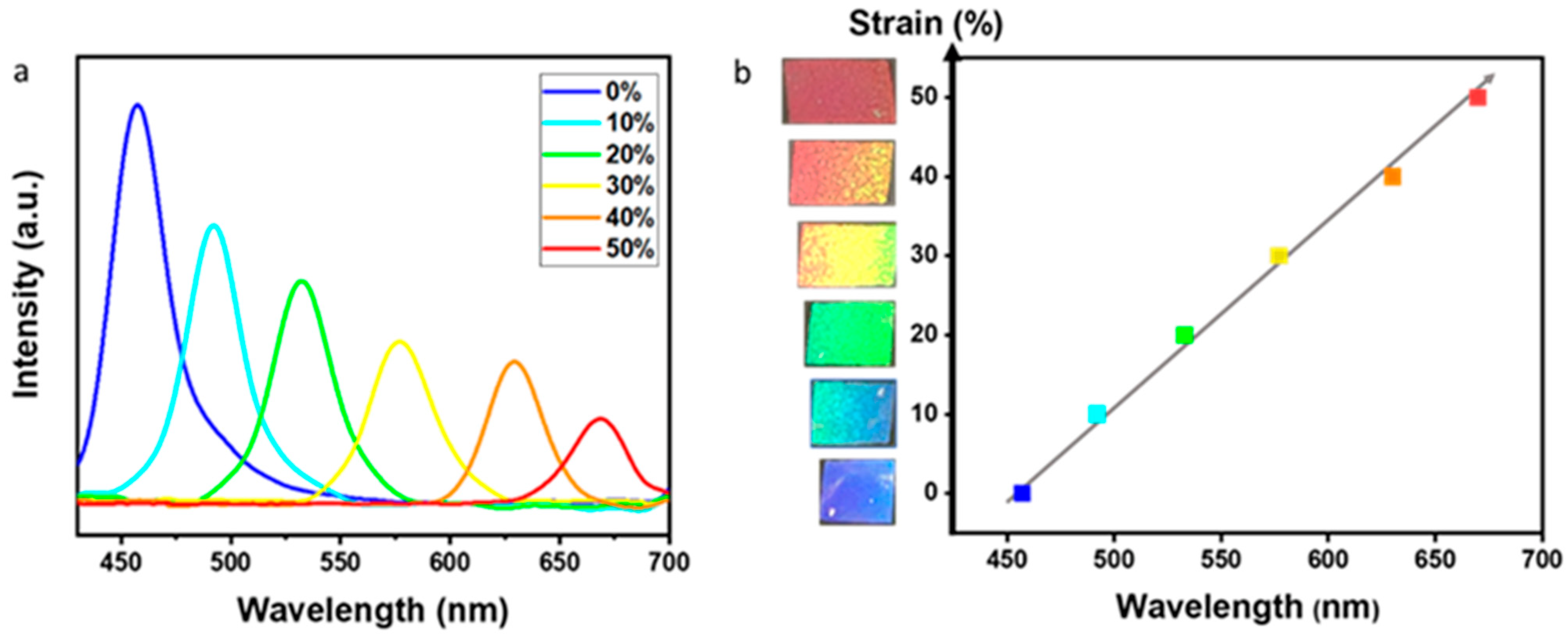
• The RGB color of the mechanochromic sensor showed different discolorations depending on the extent of displacement. B showed significant discoloration at <1 mm displacement, but the discoloration reduced for displacements > 1 mm. At 1.5–2 mm displacement, the discolorations of R and G were dominant, with R showing the largest discoloration behavior at >4 mm displacement.
• HSV also exhibited different behaviors depending on the degree of displacement. In the HSV color space, S exhibited major discoloration at an initial displacement < 1 mm, which was effective up to 3 mm. At displacements between 1–4 mm, the discoloration of H was major.
• For displacements < 1 mm, the discolorations of B and S were the most sensitive and showed the highest fitness for linear relationships, suggesting their suitability for predicting small displacements in concrete. However, owing to the influence of other colors on the small displacement as well as on large displacements, an in-depth study is required to predict the overall displacement.
• The ViT model, built with six RGB and HSV channels, exhibited a high prediction accuracy of R² = 0.997 for the measured displacement. This presents a novel methodology for predicting displacement through the discoloration of the mechanochromic sensor. However, the different discoloration characteristics depending on the angle of incidence of the mechanochromic sensor should be considered in future studies.

References

1. Lee, S.-J.; You, I.; Kim, S.; Shin, H.-O.; Yoo, D.-Y. Self-Sensing Capacity of Ultra-High-Performance Fiber-Reinforced Concrete Containing Conductive Powders in Tension. Cem. Concr. Compos. 2022, 125, 104331. [Google Scholar] [CrossRef]
2. Behnia, A.; Chai, H.K.; Shiotani, T. Advanced structural health monitoring of concrete structures with the aid of acoustic emission. Constr. Build. Mater. 2014, 65, 282–302. [Google Scholar] [CrossRef]
3. Soman, R.; Wee, J.; Peters, K. Optical fiber sensors for ultrasonic structural health monitoring: A review. Sensors 2021, 21, 7345. [Google Scholar] [CrossRef] [PubMed]
4. Fotouhi, M.; Sadeghi, S.; Jalalvand, M.; Ahmadi, M. Analysis of the damage mechanisms in mixed-mode delamination of laminated composites using acoustic emission data clustering. J. Thermoplast. Compos. Mater. 2017, 30, 318–340. [Google Scholar] [CrossRef]
5. Hoang Minh, N.H.; Kim, K.; Kang, D.H.; Yoo, Y.-E.; Yoon, J.S. Photonic crystals for dichotomous sensitivity to strain for sensor and indicator applications. ACS Appl. Nano Mater. 2024, 7, 20361–20369. [Google Scholar] [CrossRef]
6. Bae, G.; Seo, M.; Lee, S.; Bae, D.; Lee, M. Colorimetric detection of mechanical deformation in metals using thin-film mechanochromic sensor. Adv. Mater. Technol. 2021, 6, 2100479. [Google Scholar] [CrossRef]
7. Bae, G.; Seo, M.; Lee, S.; Bae, D.; Lee, M. Angle-insensitive Fabry–Perot mechanochromic sensor for real-time structural health monitoring. Adv. Mater. Technol. 2021, 6, 2100118. [Google Scholar] [CrossRef]
8. Tabatabaeian, A.; Liu, S.; Harrison, P.; Schlangen, E.; Fotouhi, M. A review on self-reporting mechanochromic composites: An emerging technology for structural health monitoring. Compos. A 2022, 163, 107236. [Google Scholar] [CrossRef]
9. Guo, Q.; Zhang, X. A review of mechanochromic polymers and composites: From material design strategy to advanced electronics application. Compos. B Eng. 2021, 227, 109434. [Google Scholar] [CrossRef]
10. Tang, C. Fundamental aspects of stretchable mechanochromic materials: Fabrication and characterization. Materials 2024, 17, 3980. [Google Scholar] [CrossRef] [PubMed]
11. Zhang, R.; Wang, Q.; Zheng, X. Flexible mechanochromic photonic crystals: Routes to visual sensors and their mechanical properties. J. Mater. Chem. C 2018, 6, 3182–3199. [Google Scholar] [CrossRef]
12. Pyeon, S.; Kim, H.; Choe, G.; Lee, M.; Jeon, J.; Kim, G.; Nam, J. Crack evaluation of concrete using mechanochromic Sensor. Materials 2023, 16, 662. [Google Scholar] [CrossRef] [PubMed]
13. ACI Committee. 224-Cracking, Causes, Evaluation, and Repair of Cracks in Concrete Structures; American Concrete Institute: Farmington Hills, MI, USA, 2007. [Google Scholar]
14. KDS 14 20 30–Serviceability design standard of concrete structure. In Korean Des. Stand. 2021.
15. Minh, N.H.; Kim, K.; Kang, D.H.; Yoo, Y.-E.; Yoon, J.S. Fabrication of robust and reusable mold with nanostructures and its application to anti-counterfeiting surfaces based on structural colors. Nanotechnology 2021, 32, 495302. [Google Scholar] [CrossRef]
16. Minh, N.H.; Kim, K.; Kang, D.H.; Yoo, Y.-E.; Yoon, J.S. An angle-compensating colorimetric strain sensor with wide working range and its fabrication method. Sci. Rep. 2022, 12, 21926. [Google Scholar] [CrossRef] [PubMed]
17. Quan, Y.-J.; Kim, Y.-G.; Kim, M.-S.; Min, S.-H.; Ahn, S.-H. Stretchable Biaxial and Shear Strain Sensors Using Diffractive Structural Colors. ACS Nano 2020, 14, 5392–5399. [Google Scholar] [CrossRef]
18. Dosovitskiy, A.; Beyer, L.; Kolesnikov, A.; Weissenborn, D.; Zhai, X.; Unterthiner, T.; Dehghani, M.; Minderer, M.; Heigold, G.; Gelly, S.; et al. An Image is Worth 16 × 16 Words: Transformers for Image Recognition at Scale. arXiv 2010, arXiv:2010.11929. [Google Scholar]
19. Lee, S.H.; Lee, S.; Song, B.C. Vision Transformer for Small-Size Datasets. arXiv 2021, arXiv:2112.13492. [Google Scholar]
20. Battisti, A.; Minei, P.; Pucci, A.; Bizzarri, R. Hue-based quantification of mechanochromism towards a cost-effective detection of mechanical strain in polymer systems. Chem. Commun. 2016, 53, 248–251. [Google Scholar] [CrossRef] [PubMed]
21. Wang, Y.; Adam, M.L.; Zhao, Y.; Zheng, W.; Gao, L.; Yin, Z.; Zhao, H. Machine Learning-Enhanced Flexible Mechanical Sensing. Nano-Micro Lett. 2023, 15, 55. [Google Scholar] [CrossRef]
22. De Castro, L.D.C.; Scabini, L.; Ribas, L.C.; Bruno, O.M.; Oliveir, O.N., Jr. Machine Learning and Image Processing to Monitor Strain and Tensile Forces with Mechanochromic Sensors. Expert Syst. Appl. 2023, 212, 118792. [Google Scholar] [CrossRef]
Figure 1. Fabrication and structure of mechanochromic sensor, where RIE, Cr, and PDMS stand for oxygen-reactive ion chamber, chromium, and polydimethylsiloxane, respectively.
Applsci 15 01066 g001
Figure 2. Color variations of mechanochromic sensor [16]; (a) reflectance spectra for different strains according to the wavelength and (b) colors and diffracted wavelengths for different strains and their comparison with theorical calculations (gray line). Note: the initial geometry of the sensor was 8 × 8 mm2.
Applsci 15 01066 g002
Figure 3. Test setup of tensile test.
Applsci 15 01066 g003
Figure 4. Graph and example images of mechanochromic sensor displacements over time (0 to 4 mm) during 400 s.
Applsci 15 01066 g004
Figure 5. Image processing workflow and ViT architecture. The 6 channels input into the Vision Transformer in this study include the R, G, B, H, S, and V channels.
Applsci 15 01066 g005
Figure 6. Changes in RGB depending on displacement.
Applsci 15 01066 g006
Figure 7. Changes in HSV depending on displacement.
Applsci 15 01066 g007
Figure 8. Result of linear curve fitting between displacement and normalized color at each stage; (a) RGB colors, (b) HSV colors.
Applsci 15 01066 g008
Figure 9. Comparison of predicted displacement using the trained ViT model on images and the measured displacement.
Applsci 15 01066 g009