Article

The Multi-Resolution Migration Imaging Method for Grounded Electrical Source Transient Electromagnetic Virtual Wavefield

by
Kailiang Lu
1,*,
Xiu Li
2,*,
Jianhua Yue
3,
Ya’nan Fan
1,
Qinrun Yang
3 and
Xiaozhen Teng
3
1
State Key Laboratory of Intelligent Construction and Healthy Operation and Maintenance of Deep Underground Engineering, China University of Mining and Technology, Xuzhou 221116, China
2
College of Geology Engineering and Geomatics, Chang’an University, Xi’an 710054, China
3
School of Resources and Geosciences, China University of Mining and Technology, Xuzhou 221116, China
*
Authors to whom correspondence should be addressed.
Appl. Sci. 2025, 15(3), 1107; https://doi.org/10.3390/app15031107
Submission received: 26 November 2024 / Revised: 19 January 2025 / Accepted: 21 January 2025 / Published: 23 January 2025

Abstract

:

Featured Application

Multi-resolution imaging of geological structures by transient electromagnetic method.

Abstract

The traditional source uses a square wave with a fixed fundamental frequency to excite transient electromagnetic (TEM) fields, with harmonic energy primarily concentrated in the low-frequency range, limiting the detection resolution of the TEM. The differential pulse, composed of two square waves with identical pulse widths but opposite polarities, concentrates harmonic energy more effectively. By adjusting the pulse width of the differential pulse, the concentration frequency band of harmonic energy can be changed, enabling multi-resolution detection of geological structures at different depths. In this study, TEM fields are excited using differential pulses of varying pulse widths during power supply. A preconditioned precise integration time-sweeping wavefield reverse transformation method is applied to interpret the virtual wavefield from the diffusion field, effectively improving the numerical accuracy and noise resistance of the virtual wavefield. Then, the finite-difference migration imaging method is used to obtain imaging profiles for differential pulses of different pulse widths, and stacking techniques are applied to acquire high-resolution characteristics of electrical interfaces at various depths. Finally, the feasibility of the method is verified through a complex geological model. By comparing the relative anomalies of square waves and differential pulses with different pulse widths, the results show that the electromagnetic anomalies for differential pulses are increased by 53.7%. Therefore, using differential pulses as the excitation source leads to higher-resolution electromagnetic responses, which in turn result in high-resolution imaging.

1. Introduction

The electrical source TEM, as an important geophysical exploration technique [1], is widely used in fields such as metal mineral exploration [2,3], coalfield geological hazard investigation [4], hydro-geophysical prospecting [5], and tunnel advance prediction [6,7] due to its high efficiency and deep detection capabilities [8,9]. However, traditional electrical source TEM primarily uses square waves (or trapezoidal waves), with fieldwork also employing triangular waves, semi-sine waves, and other waveforms [10]. Overall, these waveforms generally lack high-frequency harmonic components, making them inadequate for the fine characterization of poor geological bodies [11]. Moreover, the volume effects in TEM diffusion fields are prominent, and the resolution capability for electrical interfaces is limited when applying diffusion field-based migration imaging and inversion methods [12]. Therefore, exploring new TEM detection techniques and imaging methods is of significant value for improving the interpretation of TEM data. This study investigates a multi-resolution pre-stack migration imaging method for electrical source TEM virtual wavefields.
It is well known that traditional field sources use square waves with a fixed fundamental frequency to excite TEM fields, with harmonic energy primarily dominated by low-frequency harmonics, which limits the detection resolution [13]. To enhance the detection capabilities of the TEM, some scholars have focused on the transmitted waveform during ON-Time as a research entry point [14,15]. Liu et al. investigated the effect of different transmitted waveforms on the response of airborne electromagnetic systems, and provided the relationship between the optimal pulse width of commonly used semi-sine waves, square waves, triangular waves, and trapezoidal waves and detection time [16]. Chen et al. derived the electromagnetic field expressions for a loop source in free space for these four waveforms, studied their impact on electromagnetic detection, and pointed out that square and trapezoidal waves are suitable for ground-based electromagnetic methods, while semi-sine and triangular waves are more suitable for airborne electromagnetic methods [17]. Yin et al. conducted a detailed study on the detection capability of semi-sine and trapezoidal waves for geological targets and suggested that, based on actual exploration requirements, optimal airborne electromagnetic parameters can be designed to improve operational efficiency [18]. According to recent research, the traditional square wave lacks high-frequency harmonic components, making it difficult to fundamentally improve the detection resolution in time-domain electromagnetic methods [19]. Li et al. highlighted advancements in urban underground space imaging methods, noting that by transmitting differential pulses with varying pulse widths during the ON-Time for scanning detection, a multi-resolution TEM diffusion field can be generated, thereby enhancing the resolution of TEM detection [13]. Therefore, this paper employs differential pulse excitation to generate electromagnetic fields, and through multi-pulse scanning, enables multi-resolution detection of geological anomalies at varying depths and scales.
To achieve high-resolution imaging of TEM data, the kinematic characteristics of the wavefield can be extracted from the diffusion field based on the reverse transformation theory of TEM wavefields [20,21,22,23,24]. However, the reverse transformation equation for the virtual wavefield is a first-kind Fredholm integral equation, which is inherently ill-posed [25]. When the reverse transformation equation is linearized and discretized, the resulting coefficient matrix is severely ill-conditioned, making it difficult to accurately recover the virtual wavefield using conventional numerical methods [26]. To mitigate the ill-conditioning of the coefficient matrix, Li et al. divided the TEM diffusion field into segments based on a time sequence and applied a regularization algorithm to implement the reverse transformation of the wavefield [27]. However, this approach introduced issues with the continuity between segmented data. To address the continuity issue of the virtual wavefield, Qi et al. reduced the condition number of the ill-conditioned matrix using an over-relaxation preconditioned method and solved the virtual wavefield over the full time period with a regularized conjugate gradient algorithm [28]. Nonetheless, this method exhibited low numerical accuracy and poor noise resistance. Building on this, Qi et al. later employed a multi-window time-sweeping technique to suppress background noise interference in the virtual wavefield to some extent [12]. In addition, Xue et al. combined regularization with singular value decomposition and introduced weighting factors to obtain a stable virtual wavefield [29]. In order to further improve the numerical accuracy of the virtual wave field, some scholars have proposed a preconditioned precise integration algorithm [23,24], which transforms the solution of the ill-conditioned linear system into a stable process of infinite integration of the matrix exponential function, ensuring high computational efficiency while maintaining accuracy. Furthermore, by incorporating the multi-window time-sweeping technique into the preconditioned precise integration algorithm [23], the noise resistance of the virtual wavefield was significantly enhanced.
However, the coherent axes of the virtual wavefield typically reflect the characteristics of shallow formations more accurately. As subsurface structures become increasingly complex, the coherent axes of the virtual wavefield in deeper regions cannot reliably represent the stratigraphic morphology, necessitating the use of migration imaging methods for spatial positioning [30]. Li et al. used the three-dimensional boundary element method combined with the Kirchhoff method to achieve the surface extension of the virtual wavefield [31]. Xue et al. employed deconvolution techniques and wavelet compression to enhance the vertical resolution of migration imaging [32]. Qi et al. based on a full time-domain virtual wavefield, utilized Kirchhoff integral migration, inverse synthetic aperture, and deconvolution techniques to achieve high-resolution pseudo-seismic three-dimensional imaging results [12]. Fan et al., drawing on the Born approximation imaging method from the field of seismic exploration, achieved rapid imaging of the virtual wavefield [22]. By processing electromagnetic data from coal seam goaf areas, they successfully identified electrical interface features. Xue et al. used virtual wavefields to achieve full-waveform inversion imaging, which not only improves vertical resolution but also provides accurate parameter estimation [26]. To better address the migration imaging problem in media with significant lateral velocity variations, Lu et al., starting from the time-domain wave equation, extrapolated the first-order approximation of the upgoing wave equation to obtain a time–space domain wavefield recursion formula [33]. Using the finite difference method, they solved the wavefield in subsurface spaces and obtained accurate electrical interface features. While all these imaging methods provide information on electrical interfaces within formations, they are limited by the resolution of the source field and struggle to achieve multi-resolution imaging from shallow to deep regions.
In summary, this paper first transmits multiple differential pulses with varying pulse widths during the ON-Time period to obtain a multi-resolution TEM diffusion field. Then, a preconditioned precise integration wavefield reverse transformation method is employed to extract the virtual wavefield from the diffusion field. Finally, pre-stack migration imaging technology is applied to obtain electrical interface characteristics from shallow to deep layers, effectively addressing the challenge of multi-resolution detection.

2. Differential Pulse Spectrum Analysis and 3D Forward Modeling

2.1. Differential Pulse Spectrum Analysis

Figure 1a and Figure 2a show waveforms of different pulse widths and their corresponding spectra. The pulse widths of the square wave and differential pulse are 0.6 ms, 1.0 ms, 2.5 ms, 5.0 ms, and 10.0 ms, respectively. Figure 1b and Figure 2b present the normalized spectra of the square wave and differential pulse, where hollow circles represent the cutoff frequencies, and solid circles represent the dominant frequencies. As shown in Figure 1, the square wave is a broadband waveform, but its harmonic energy is mainly concentrated in the low-frequency range, lacking high-resolution harmonic components. In contrast, Figure 2 shows that the differential pulse consists of two square waves with identical pulse widths but opposite polarities, with its harmonic energy concentrated near the dominant frequency. Compared to the spectrum of a square wave with the same pulse width, the differential pulse exhibits a higher cutoff frequency, indicating a richer content of high-frequency harmonics. As the pulse width of the differential pulse decreases, both the dominant and cutoff frequencies shift toward the high-frequency range. Given the varying dominant frequencies and the concentrated harmonic energy of differential pulses with different pulse widths, this study uses multiple differential pulses to scan subsurface spaces, enabling multi-resolution imaging from shallow to deep layers.
To investigate the relationship between differential pulse width, dominant frequency, and detection depth, this paper presents approximate curves for pulses with widths ranging from 10 µs to 100 ms, along with their corresponding dominant frequencies and detection depths. Figure 3a shows the dominant frequency curve for differential pulses of different pulse widths, where it is evident that as the pulse width increases, the dominant frequency decreases. Figure 3b displays the approximate curves of pulse width versus detection depth, derived using the skin depth formula under different uniform half-space conductivity conditions. It can be observed that detection depth increases with pulse width, and the smaller the conductivity of the uniform half-space, the greater the detection depth.

2.2. 3D Forward Modeling of Differential Pulse

For the 3D forward modeling of differential pulse, this study adopts the unstructured tetrahedral vector finite element method. To achieve efficient numerical simulations, the second-order backward differentiation formula (BDF2) is employed during the ON-Time stage, while the shift-and-invert Krylov (SAI-Krylov) subspace method is used during the OFF-Time stage.
For a given computational domain Ω, neglecting the displacement current, Maxwell’s equations can be expressed in the following form [34]:
× e = b t ,
× μ 0 1 b σ e = J s t .
where e represents the electric field intensity ( V · m 1 ), b denotes the magnetic flux density (T), μ 0 is the magnetic permeability of free space ( H · m 1 ), J s represents the current density ( A · m 2 ), and σ is the electrical conductivity of the subsurface ( S · m 1 ). At infinity, the first-type boundary condition is applied in this study.
By discretizing the space using an unstructured tetrahedral mesh, eliminating the magnetic flux density b from Equation (1) and (2), and applying the Galerkin method, the governing equation for the electric field can be derived as follows:
V   × N i × N j d V e + V   μ 0 σ N i N j d V e t = V   μ 0 N i N j d V J s t .
where N i and N j are the interpolation basis functions within the element. Applying the BDF2 to the derivative terms in Equation (3) yields the following:
V   × N i × N j d V e n + V   μ 0 σ N i N j d V 3 e n 4 e n 1 + e n 2 2 Δ t + V   μ 0 N i N j d V 3 J s n 4 J s n 1 + J s n 2 2 Δ t = 0 .
where e n and J s n represent the electric field intensity and current density at time step n, respectively. In this study, the matrices are defined as follows: M c u r l = V   × N i × N j d V , M σ = V   μ 0 σ N i N j d V , M i n n e r = V   μ 0 N i N j d V . Thus, the electric field intensity during the ON-Time can be solved using the following equation [35]:
2 Δ t M c u r l + 3 M σ e n = M σ 4 e n 1 e n 2 M i n n e r 3 J s n 4 J s n 1 + J s n 2 .
After the current is turned off (OFF-Time), J s in Equation (3) becomes zero and can be rewritten as follows:
e t = M σ 1 M c u r l e ,
Using the SAI-Krylov subspace method to solve Equation (6) [36,37,38], the approximate solution can be expressed in the following form:
e t e m t = V m e t γ H m 1 I e 0 2 e 1 ,
where m is the order of the SAI-Krylov subspace, γ is the shift parameter, I is the identity matrix, and e 0 represents the electric field intensity at the time of current shutdown. The vector e 1 = 1,0 , , 0 m T . V m and H m are the basis vector matrix and the projection matrix, respectively, which can be solved using the Arnoldi algorithm [39].

2.3. Validation of Magnetic Flux Density for Differential Pulse

In this study, a differential pulse with a pulse width of 20 ms is used to validate the 3D forward modeling method. The resistivity of the air layer is set to 106 Ω∙m, and the resistivity of the homogeneous half-space is 200 Ω∙m. The grounded wire has a length of 1 km and is placed along the x-axis, with the coordinates of the two endpoints at (−500 m, 0 m, 0 m) and (500 m, 0 m, 0 m), respectively. The current intensity is 10 A. The coordinates of the four measurement points are (100 m, 100 m, 0 m), (200 m, 200 m, 0 m), (500 m, 500 m, 0 m), and (1 km, 1 km, 0 m). Since the current analysis primarily focuses on the electromagnetic data during the OFF-Time stage, the sampling time ranges from 1 µs to 100 ms after the current is turned off, with a total of 51 time channels logarithmically spaced.
Figure 4a shows the z-component of the magnetic flux density, where the dashed line represents the 1D results, and the circles represent the 3D results. The two are in good agreement. Figure 4b presents the relative error curve, with the overall numerical error being less than 5%, which validates the accuracy of the 3D numerical method used in this study.

3. Preconditioned Precise Integration Time-Sweeping Method

The virtual wavefield can be interpreted from the TEM diffusion field, enabling high-resolution migration imaging of electrical interfaces in subsurface formations. In this study, the precise integration method is employed to transform the solution of the ill-conditioned linear system into an infinite integral of the matrix exponential function, significantly improving the numerical accuracy of the virtual wavefield. Considering the presence of background noise in field data, a multi-window time-sweeping technique is introduced based on the preconditioned precise integration method, effectively enhancing the noise resistance of the wavefield reverse transformation method.

3.1. Preconditioned Precise Integration Algorithm

The relationship between the TEM diffusion field and the virtual wavefield is as follows [20,27]:
f r , t = 1 2 π t 3 0   τ exp τ 2 4 t u r , τ d τ ,
In Equation (8), f and u represent the diffusion field and the virtual wavefield, respectively, while t and τ represent the diffusion field time and virtual time, respectively. The exp denotes the exponential function. Equation (8) is a Fredholm integral equation of the first kind, which exhibits typical ill-posedness. Its linearization and discretization can yield the following:
f t i = j = 1 n   k i , j u τ j ,
where k i , j = 1 / π t i e x p τ 2 / 4 t i τ j 1 τ j , and Equation (9) can be expressed as the following linear equation system:
K u = f .
The system of linear Equation (10) exhibits severe ill-conditioning. In this paper, we solve the virtual wavefield u using the preconditioned precise integration method. Since the precise integration method requires the coefficient matrix K to be symmetric and positive definite, Equation (10) is rewritten in the following form:
K T K u = K T f ,
Let the matrix A = K T K . By left-multiplying both sides of Equation (11) by the preconditioned matrix Q and setting u = P y , then
Q A P y = Q K T f ,
Equation (12) can be simplified into the following form:
M y = b ,
where M = Q A P , b = Q K T f . By applying the preconditioned precise integration method, the solution of linear Equation (13) can be expressed in the following iterative form [23]:
y k = i = 0 k 1   I + exp 2 k i 1 ζ M F ( ζ ) b y k + 1 = I + exp 2 k ζ M y k , k = 0,1 , 2 , ,
the ζ represents the integration step size, and F ( ζ ) is expressed as follows:
F ζ = ζ I + ( M ζ ) / 2 + ( M ζ ) 2 / 6 + ( M ζ ) 3 / 24 .
After solving for y using the iterative Formula (14), the virtual wavefield can be obtained by u = P y .

3.2. Time-Sweeping Wavefield Reverse Transformation Method

To suppress interference and highlight anomalous information, this paper introduces a multi-window time-sweeping technique based on the preconditioned precise integration algorithm. First, different sweeping time windows are set, and the virtual wavefield is computed for each window. Then, a correlation analysis is performed between the virtual wavefield of each window and that of the full time period. If the correlation coefficient exceeds the predefined threshold, the corresponding virtual wavefields are combined through correlation summation to obtain the virtual wavefields for different windows. Finally, by stacking the virtual wavefields from different windows, the wavefield information for the entire virtual time profile is obtained [40]. The schematic diagram of the process is shown below [23] (Figure 5).

4. The Multi-Resolution Pre-Stack Migration Imaging Method

In cases where the formation dip is small and the geological structure is simple, the phase axis of the virtual wavefield can intuitively reflect the characteristics of the geological structure. However, for complex geological structures, the phase axis of the virtual wavefield in deeper regions cannot accurately represent the formation morphology, requiring the use of migration imaging methods to spatially position it accurately.

4.1. The Finite-Difference Migration Imaging Method

In a Cartesian coordinate system, the governing equation for the wavefield in the passive region is as follows [33]:
2 u 1 v 2 2 u t 2 = 0 ,
In this paper, upgoing waves are used for migration imaging, Equation (16) is rewritten as a two-dimensional wave equation:
2 u x 2 + 2 u z 2 = 1 v 2 2 u t 2 .
By applying a coordinate transformation to Equation (17), let x = x , z = z , and t = t + z / v . Since the wave field remains invariant under the change of coordinates, we have u x , z , t = u x , z , t . Based on this, the following expression can be derived:
2 u x 2 = 2 u x 2 2 u z 2 = 2 u z 2 + 2 v 2 u z t + 1 v 2 2 u t 2 2 u t 2 = 2 u t 2 .
Substituting Equation (18) into Equation (16) yields the wave equation in the floating coordinate system:
2 u x 2 + 2 v 2 u z t + 2 u z 2 = 0 ,
By performing a Fourier transform on x and t in Equation (19), the first-order approximation equation can be obtained [33]:
2 u z t + v 4 2 u x 2 = 0 .
In the above equation, the velocity v can either be a constant or a function of x and z , denoted as v x , z .
Assume that Equation (20) exists in the spatial domain Ω < x < , 0 t T , 0 z < Z , with the following mixed boundary conditions given:
u x , z , T = 0 x , z , T t = 0 u x , z = 0 , t = φ x , t u x , Z , t = 0 .
where u x , z = 0 , t = φ x , t represents the wave field observed at the surface. By solving the above partial differential equation, the wave field values u x , z , t of the upgoing waves at any point in the subsurface x , z > 0 can be obtained.
In this paper, the Crank–Nicolson symmetric implicit difference scheme is employed, as illustrated in Figure 6.
Next, the following notation is used to derive the equation:
u i , j n = u i x , n z , j t = u x , z , t δ t u i , j + 1 / 2 n = u i , j + 1 n u i , j n / t δ x x u i , j + 1 / 2 n = u i + 1 , j + 1 / 2 n 2 u i , j + 1 / 2 n + u i 1 , j + 1 / 2 n / x 2 ,
where x and z are the spatial steps in the x and z directions, respectively, and t is the time step. For the central point in Figure 6, the wavefield is denoted as u i , j + 1 / 2 n + 1 / 2 . Let u = u i , j + 1 / 2 n + 1 / 2 , u z = u i , j + 1 / 2 n + 1 u i , j + 1 / 2 n z , then Equation (20) can be simplified as
2 u z t = 1 z t u i , j + 1 n + 1 u i , j n + 1 u i , j + 1 n + u i , j n .
For the 2 u x 2 , let u = u i , j + 1 / 2 n + 1 + u i , j + 1 / 2 n / 2 , then
2 u x 2 = 1 2 x 2 u i + 1 , j + 1 / 2 n + 1 2 u i , j + 1 / 2 n + 1 + u i 1 , j + 1 / 2 n + 1 + u i + 1 , j + 1 / 2 n 2 u i , j + 1 / 2 n + u i 1 , j + 1 / 2 n ,
In summary, Equation (20) can be written in the following form:
u i , j + 1 n + 1 u i , j n + 1 u i , j + 1 n + u i , j n = v z t 8 x 2 u i + 1 , j + 1 / 2 n + 1 2 u i , j + 1 / 2 n + 1 + u i 1 , j + 1 / 2 n + 1 + u i + 1 , j + 1 / 2 n 2 u i , j + 1 / 2 n + u i 1 , j + 1 / 2 n ,
Let α = v z t 8 x 2 , δ ^ t + = t δ t + , δ t + u i , j + 1 / 2 n = u i , j + 1 n u i , j n / t , δ ^ x x = x 2 δ x 2 ; the discrete expression of Equation (25) can then be simplified as follows:
δ ^ t + + α δ ^ x x u i , j + 1 / 2 n + 1 = δ ^ t + α δ ^ x x u i , j + 1 / 2 n .
To obtain the expression for the integer-point sampling, let u i , j + 1 / 2 n = u i , j + 1 n + u i , j n / 2 and u i , j + 1 / 2 n + 1 = u i , j + 1 n + 1 + u i , j n + 1 / 2 . Then, Equation (26) can be transformed into
I α δ ^ x x u i , j n + 1 = I + α δ ^ x x u i , j + 1 n + 1 + I + α δ ^ x x u i , j n I α δ ^ x x u i , j + 1 n ,
After rearranging Equation (27), we obtain
( I + 2 α ) u i , j n + 1 α u i + 1 , j n + 1 α u i 1 , j n + 1 = ( I 2 α ) u i , j + 1 n + 1 + u i , j n + α u i + 1 , j + 1 n + 1 + u i + 1 , j n + α u i 1 , j + 1 n + 1 + u i 1 , j n ( I + 2 α u i , j + 1 n α u i + 1 , j + 1 n α u i 1 , j + 1 n ,
where i = 1,2 , , n x ; j = 1,2 , , n t , and n x represents the number of nodes in the x -direction, and n t is the number of time samples at each measurement point.
To express Equation (28) in matrix form
A u j n + 1 = B u j + 1 n + 1 + u j n A u j + 1 n ,
where u j n is the wavefield vector along the x-direction at the depth layer z = n z and time layer t = j t ; u j + 1 n , u j n + 1 , and u j + 1 n + 1 represent the corresponding wavefield vectors at the respective layers. The expressions for matrices A , B , and vectors u j n + 1 , u j + 1 n + 1 , u j n , and u j + 1 n are as follows:
A = 1 + 2 α α α 1 + 2 α α α 1 + 2 α α α 1 + 2 α n x × n x ,
B = 1 2 α α α 1 2 α α α 1 2 α α α 1 2 α n x × n x ,
u j n + 1 = u 1 , j n + 1 , u 2 , j n + 1 , , u i , j n + 1 , , u n x , j n + 1 T u j + 1 n + 1 = u 1 , j + 1 n + 1 , u 2 , j + 1 n + 1 , , u i , j + 1 n + 1 , , u n x , j + 1 n + 1 T u j n = u 1 , j n , u 2 , j n , u i , j n , , u n x , j n T u j + 1 n = u 1 , j + 1 n , u 2 , j + 1 n , , u i , j + 1 n , , u n x , j + 1 n T .
The vectors u j n and u j + 1 n in Equation (29) represent the TEM virtual wavefields observed at the surface during the first downward extrapolation. During reverse extrapolation, the wavefield at the surface receiver points can be treated as the source. Thus, when calculating u j n + 1 , it is known that u j + 1 n + 1 is zero. Therefore, as long as matrix A is invertible, Equation (29) is solvable, that is:
u j n + 1 = A 1 B u j n u j + 1 n .
Since A is a diagonally dominant matrix and α is always greater than zero, we have 1 + 2 α > 2 α , which implies that d e t A 0 . Therefore, the matrix A is invertible [33].
The wavefield at the grid nodes in the subsurface can be extrapolated downward using the aforementioned method. Subsequently, the wavefield values at the grid nodes, corresponding to a travel time of 2 z / v , are extracted as imaging data. These data are then arranged in both the horizontal and depth directions, ultimately yielding the imaging results of the electrical interface.

4.2. The Correlation Stacking Method for Differential Pulse Imaging

The requirements for imaging resolution in TEM are becoming increasingly stringent. However, previous research has primarily focused on data processing and interpretation methods, often neglecting the impact of the field source on detection capabilities. Due to the resolution limitations inherent to the field source, simply optimizing data processing and interpretation methods is insufficient for fundamentally enhancing the ability to identify electrical interfaces. In this study, we propose a multi-resolution imaging approach using differential pulses with varying pulse widths to image electrical interfaces at different depths in the subsurface, which effectively enhances the detection capabilities of the TEM method.
For a given survey line, n differential pulses with different pulse widths are first used to excite the TEM field, resulting in n sets of diffusion field data. Next, the virtual wavefields are extracted from these n diffusion fields using the preconditioned precise integration time-sweeping algorithm. Then, the finite-difference method is applied to obtain the migration imaging of these n virtual wavefields. Finally, the migration images with different resolutions are stacked to produce a high-resolution imaging profile. Since the migration imaging is performed prior to the “stacking” process, this method is referred to as multi-resolution pre-stack migration imaging of TEM virtual wavefields, as illustrated in Figure 7.

5. Numerical Examples

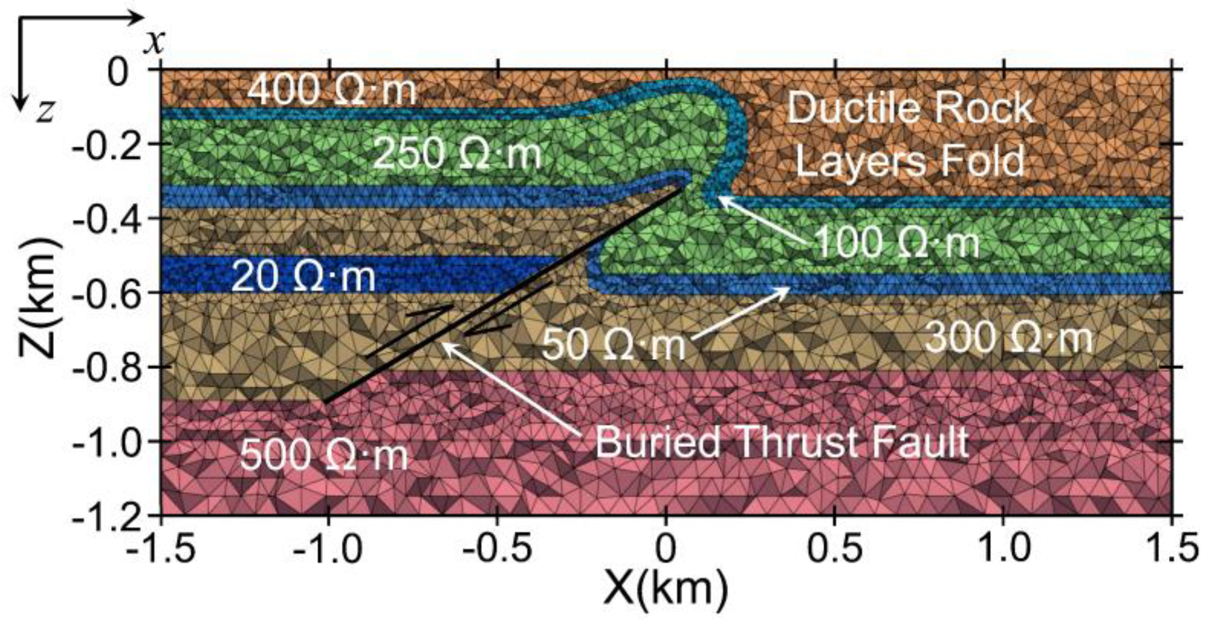
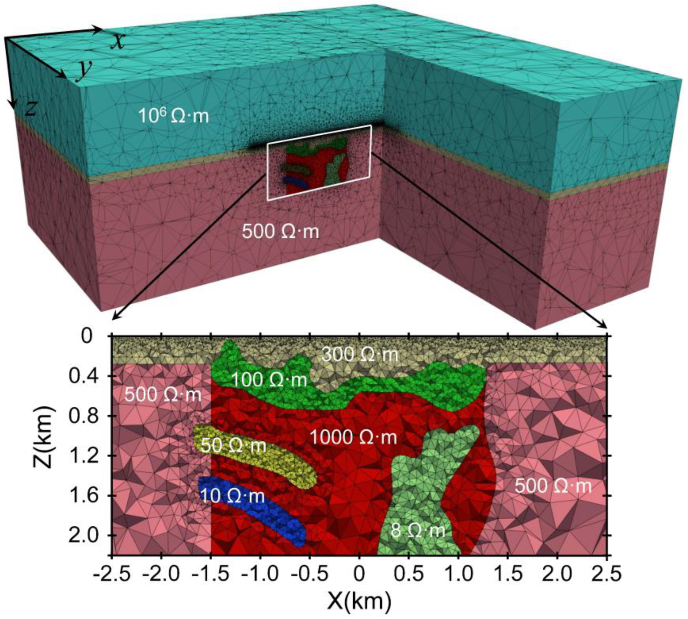
5.1. Buried Thrust Fault Model

To validate the imaging workflow shown in Figure 7, a buried thrust fault model is employed first. The schematic diagram of the model and the resistivity of the strata are shown in Figure 8. The geological model primarily consists of two main structures: a shallow ductile rock layer fold and a deep blind thrust fault. A grounded wire, 4 km in length, is used as the transmitter. The coordinates of the two endpoints of the transmitter are (−2 km, 0 m, 0 m) and (2 km, 0 m, 0 m), respectively. The receiver line, parallel to the transmitter, is 3 km long, with endpoints at (−1.5 km, 100 m, 0 m) and (1.5 km, 100 m, 0 m). The model includes three low-resistivity layers with resistivities of 100 Ω∙m, 50 Ω∙m, and 20 Ω∙m. Based on the qualitative relationship between the differential pulse width and detection depth, and through extensive experiments, differential pulses with pulse widths of 0.4 ms, 2 ms, and 5 ms are selected as the transmitted waveforms.
Figure 9 presents the computational results for square waves with pulse widths of 0.4 ms, 2 ms, and 5 ms. Figure 9a,d,g show bz with low-resistivity anomalies, while Figure 9b,e,h show bz without anomalies. Figure 9c,f,i show the corresponding relative anomaly contours. From the relative anomaly contours, it can be observed that the shallow electromagnetic anomalies for square waves with different pulse widths are more pronounced. Although increasing the pulse width enhances the deep subsurface electromagnetic anomalies, they remain relatively weak.
Figure 10 presents the computational results for differential pulses with pulse widths of 0.4 ms, 2 ms, and 5 ms. It can be observed that it is also difficult to directly identify electromagnetic anomalies from the diffusion fields (Figure 10a,d,g). Therefore, relative anomalies are used for illustration (Figure 10c,f,i). When the pulse width is 0.4 ms, Figure 10c clearly reveals the shallow anomalous features of the ductile rock layer fold. As the pulse width increases to 2 ms, the shallow anomalous features of the ductile rock layer fold gradually weaken, while the deeper anomalous features become more prominent (Figure 10f). When the pulse width increases to 5 ms, the anomalous features of the buried thrust fault become more distinct, while the anomalies associated with the ductile rock layer fold become weaker (Figure 10i). By exciting the TEM field with differential pulses of varying pulse widths, electromagnetic anomalies from geological bodies at different depths can be obtained.
Comparing Figure 9 and Figure 10, it is observed that the early amplitude of the diffusion fields excited by square waves and differential pulses with the same pulse width is nearly identical, while the amplitude of the square wave diffusion field is stronger in the later stage. However, as shown by the relative anomaly contour plots, the relative anomalies induced by the differential pulse are more pronounced, with an improvement of 53.7% over the square wave (Figure 9c and Figure 10c). The following sections will further compare the virtual wavefields and migration imaging results of square waves and differential pulses with different pulse widths.
To simulate field data and perform imaging of electrical interfaces, 5% random noise was first added to the diffusion field, followed by the application of wavelet transform methods to remove the noise interference from the diffusion field. Finally, a precise pre-processing integration method was applied to extract the virtual wavefield from the diffusion field, as shown in Figure 11. It is observed that, with the increase in square wave pulse width, there are no significant changes in the shallow subsurface features, while the deep subsurface features gradually intensify, though they remain insufficiently pronounced.
Figure 12 shows the virtual wavefield corresponding to differential pulses with different pulse widths. Figure 12a,b clearly depict the interface features of the shallow ductile rock layer fold, but it is difficult to capture the interface information of the deep buried thrust fault. As the pulse width increases to 5 ms, Figure 12c reveals the interface information of the deeper strata.
As previously mentioned, the virtual wavefield’s phase axes can only intuitively reflect the morphology of the shallow strata and cannot accurately depict the characteristics of deeper formations. Therefore, migration imaging is required to correctly position these features spatially.
Figure 13 presents the migration imaging results for square waves with different pulse widths. It can be observed that the geometric characteristics of the shallow subsurface layers show little change. As the pulse width of the square wave increases, the deep subsurface features are somewhat enhanced, but the stratigraphic interfaces remain difficult to clearly delineate.
Figure 14 shows the migration imaging for differential pulses with different pulse widths. It can be observed that the migration imaging results for differential pulses with varying pulse widths effectively characterize the interface morphology of strata at different depths (Figure 14a–c). By stacking the imaging results from different differential pulses, a high-resolution imaging profile can be obtained (Figure 14d), where the red dashed line represents the theoretical model’s electrical interface. However, due to effects such as volume effects, there are discrepancies between the migration imaging of the shallow fold and the theoretical model.

5.2. Complex Geological Model

Figure 15 shows the complex geological model. The resistivity of the air layer is set to 106 Ω∙m, and the resistivity of the homogeneous half-space is 500 Ω∙m. The surface consists of Quaternary sediments with a resistivity of 300 Ω∙m; the shallow geothermal reservoir has a resistivity of 100 Ω∙m, while the deep geothermal reservoir has resistivities of 50 Ω∙m and 10 Ω∙m, and the resistivity of the geothermal fluid is 8 Ω∙m. The length of these geological anomalies in the y-direction is 1 km. The grounded wire source used in this study is 6 km in length, with endpoints at coordinates (−3 km, −100 m, 0 m) and (3 km, −100 m, 0 m). The receiver line is parallel to the transmitter, with an offset of 200 m and a point spacing of 20 m. The endpoints of the receiver line are located at (−2.5 km, 100 m, 0 m) and (2.5 km, 100 m, 0 m). Based on the qualitative relationship between differential pulse width and detection depth, and through extensive experiments, differential pulses with pulse widths of 1 ms, 4 ms, and 12 ms were selected as the transmitted waveforms.
Figure 16 presents the computational results for differential pulses with pulse widths of 1 ms, 2 ms, 4 ms, 8 ms, and 12 ms. Figure 16a,d,g,j,m show bz with low-resistivity anomalies for differential pulses of varying widths, while Figure 16b,e,h,k,n show bz without anomalies for the same pulses. Since the electromagnetic response characteristics of differential pulses with different pulse widths cannot be directly reflected in bz, relative anomalies are used for characterization. As seen in Figure 16c, when the 1 ms differential pulse is used to excite the electromagnetic field, only the shallow geothermal reservoir shows prominent anomalous features. As the pulse width increases to 4 ms, the electromagnetic anomaly of the shallow geothermal reservoir weakens, while the anomalous features of the deeper geothermal reservoir with a resistivity of 50 Ω∙m and the shallow geothermal fluid become more pronounced. When the pulse width increases to 12 ms, the deeper geothermal reservoir with a resistivity of 10 Ω∙m and the deeper geothermal fluid show distinct anomalous features, while other low-resistivity anomalies are less prominent.
Figure 17 shows the virtual wavefields for differential pulses with different pulse widths. It can be observed that differential pulses with smaller pulse widths provide higher resolution for the electrical interfaces of shallow strata. As the pulse width increases, the resolution of the shallow strata gradually decreases, while the resolution of the electrical interfaces of deeper strata improves.
Figure 18 presents the migration imaging results for differential pulses with different pulse widths. Figure 18a–e correspond to differential pulses with pulse widths of 1 ms, 2 ms, 4 ms, 8 ms, and 12 ms, respectively, Figure 18f shows the stacked imaging profile. The figures demonstrate that using differential pulses with varying pulse widths to excite the electromagnetic field allows for high-resolution imaging of electrical interfaces at different depths. The stacked migration imaging clearly delineates the electrical interface features from shallow to deep strata. However, due to volume effects, discrepancies exist between the migration imaging of the deep geothermal reservoir with a resistivity of 10 Ω∙m and the geothermal fluid, and the theoretical model. Additionally, it can be observed that the migration imaging method for TEM virtual wavefields struggles to accurately depict vertical electrical interfaces.

6. Conclusions

This paper proposes the multi-resolution pre-stack migration imaging method of the virtual wave field in TEM exploration with electrical sources. By exciting the electromagnetic field with differential pulses of varying pulse widths, the detection resolution of TEM can be effectively improved. To capture the electrical interface characteristics of the subsurface layers, this study employs the preconditioned precise integration scanning wave field inverse transformation method to extract the virtual wave field from the diffusion field. The finite-difference method is then used for migration imaging, and the migration results from different differential pulses are stacked to obtain a high-resolution imaging profile from shallow to deep regions. The following conclusions are drawn:
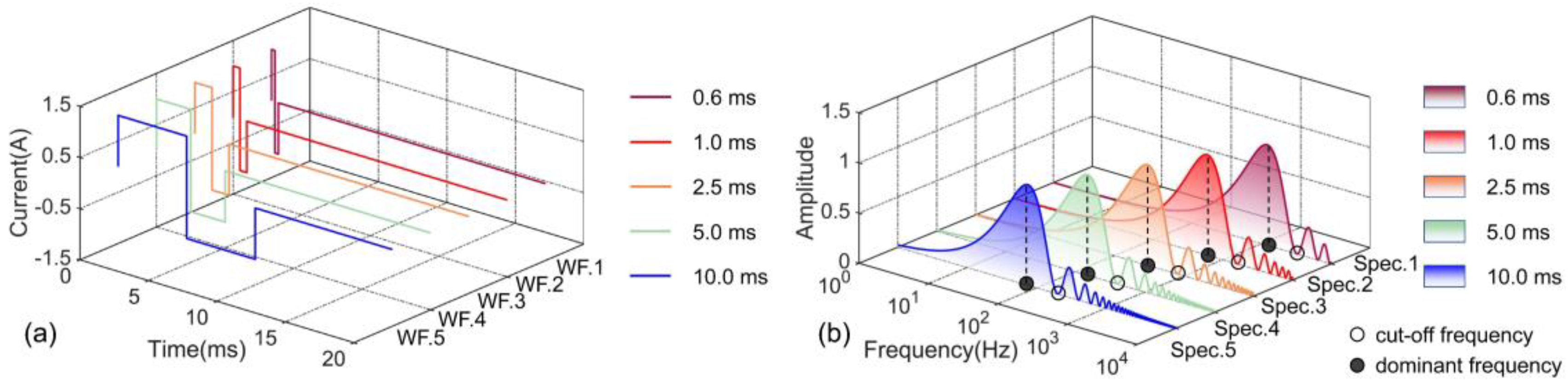
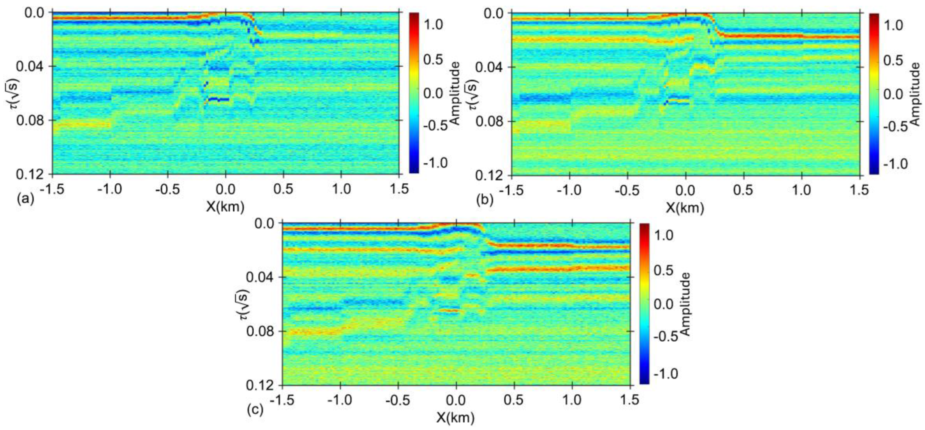
  • When square waves are used as the excitation waveform, the dominance of low-frequency harmonics hinders the achievement of high-resolution detection. In contrast, differential pulses effectively enhance high-frequency harmonics, thereby mitigating the impact of low-frequency harmonics on detection performance.
  • Based on the buried thrust fault model, square waves and differential pulses with different pulse widths were used as excitation sources. From the relative anomaly maps of bz, it is observed that the anomaly response increased by 53.7%, indicating that differential pulses provide higher detection resolution.
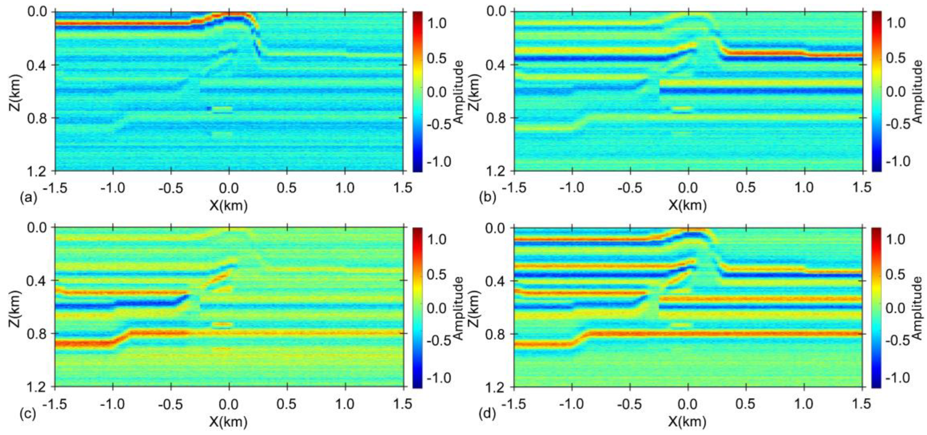
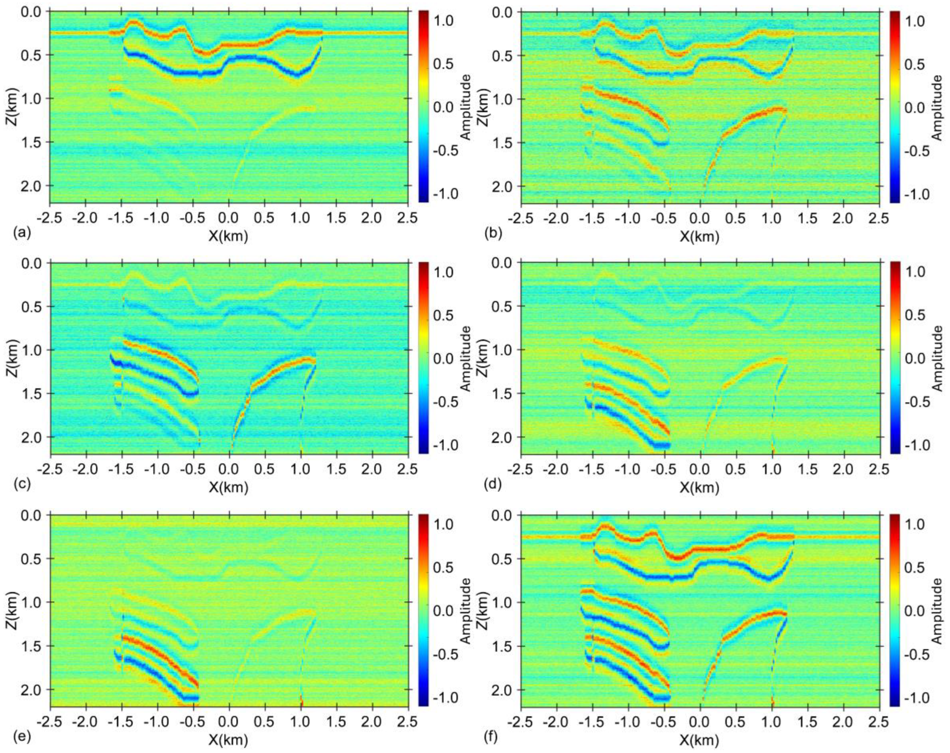
  • The TEM diffusion field exhibits a stronger volumetric effect. Converting it into a virtual wavefield can effectively mitigate the impact of the volumetric effect. However, the virtual wavefield cannot accurately represent the subsurface features, and it is necessary to apply migration imaging methods to obtain the geometric shapes of the stratigraphic interfaces.
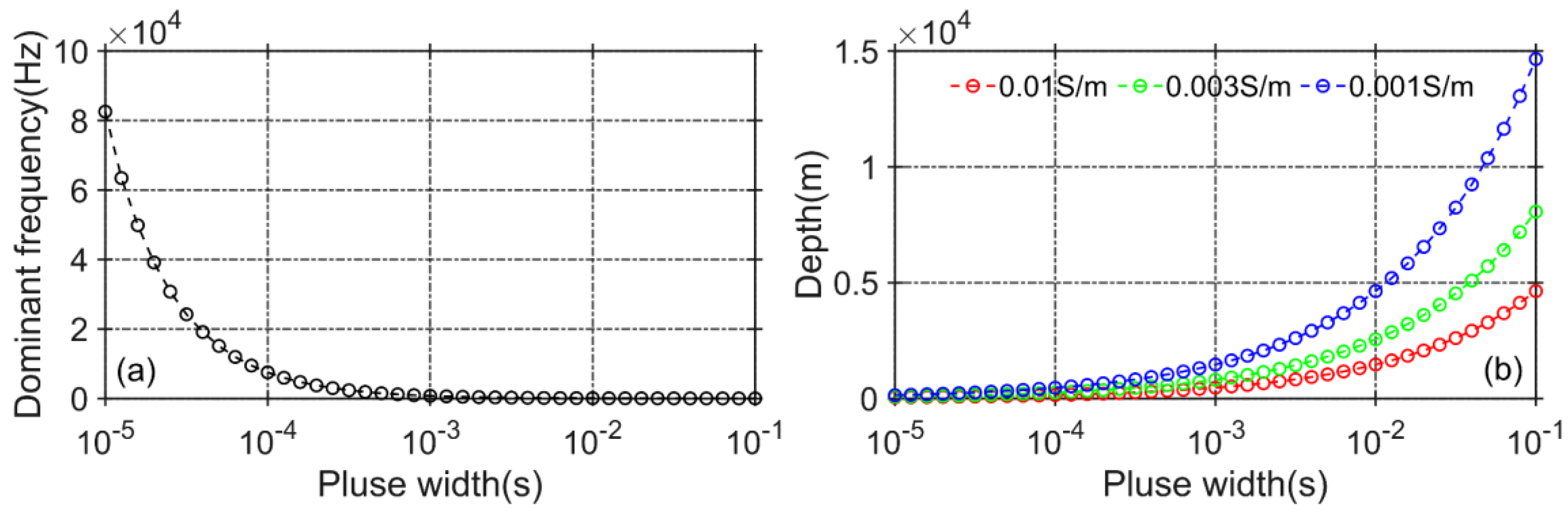
  • Square waves with different pulse widths can effectively reflect the geometric characteristics of the shallow subsurface layers. As the pulse width of the square wave increases, although the resolution of the deep subsurface layers improves to some extent, the enhancement remains limited.
  • Imaging results from the buried thrust fault model and the complex geological model demonstrate that differential pulses enable multi-resolution detection across different depth ranges, which can subsequently be used to obtain high-resolution imaging through correlation stacking.
  • This paper investigates the use of differential pulses with varying pulse widths to excite transient electromagnetic fields, and employs migration imaging methods to image the interfaces of geological anomalies. Future research will focus on developing resistivity imaging methods using differential pulses with different pulse widths.
  • This study primarily addresses the fundamental theoretical research on transient electromagnetic multi-resolution detection. The corresponding equipment is currently in the final stage of debugging. We plan to conduct the first experimental validation once the equipment is completed, with the experimental validation expected to begin in August 2025. At that time, a systematic evaluation of the proposed method will be conducted.
In summary, this research provides guidance for time-domain electromagnetic exploration and data interpretation. Future studies should explore how to design the optimal combination of differential pulse waveforms tailored to specific geological structures. Since this study primarily focuses on the foundational theoretical work and the development of the proposed method, the next step will be to apply the presented data processing techniques to field data to further validate the feasibility of the method.

Author Contributions

Writing—original draft, validation, methodology, and formal analysis, K.L.; writing—review and editing, funding acquisition, and conceptualization: K.L., X.L. and J.Y.; review and editing, analysis and interpretation: Y.F., Q.Y. and X.T. All authors have read and agreed to the published version of the manuscript.

Funding

This research was funded by National Natural Science Foundation of China (Grant No. 42230811, 42404154), Basic Research Program of Jiangsu (Grant No. BK20241672), and Jiangsu Funding Program for Excellent Postdoctoral Talent.

Institutional Review Board Statement

Not applicable.

Informed Consent Statement

Not applicable.

Data Availability Statement

The raw data supporting the conclusions of this article will be made available by the authors on request.

Acknowledgments

The authors would like to thank China University of Mining and Technology for providing the facilities required for this research. The authors also appreciate the constructive feedback from reviewers and colleagues, which helped improve the quality of this paper.

Conflicts of Interest

The authors declare no conflicts of interest.

References

  1. Xue, G.Q.; Wu, X.; Chen, K.; Lei, K.X.; Zhao, Y.; Lv, P.F.; Shi, J.J. An analysis of the shadow effect for the short-offset transient electromagnetic method. J. Appl. Geophys. 2022, 206, 104833. [Google Scholar] [CrossRef]
  2. Fournier, D.; Kang, S.; McMillan, M.; Oldenburg, D. Inversion of airborne geophysics over the DO-27/DO-18 kimberlites-Part 2: Electromagnetics. Interpretation 2017, 5, T313–T325. [Google Scholar] [CrossRef]
  3. Di, Q.Y.; Xue, G.Q.; Yin, C.C.; Li, X. New methods of controlled-source electromagnetic detection in China. Sci. China Earth Sci. 2020, 50, 1219–1227. [Google Scholar] [CrossRef]
  4. Jiang, Z.H.; Liu, L.B.; Liu, S.C.; Yue, J.H. Surface-to-Underground Transient Electromagnetic Detection of Water-Bearing Goaves. IEEE Trans. Geosci. Remote Sens. 2019, 57, 5303–5318. [Google Scholar] [CrossRef]
  5. Gottschalk, L.; Knight, R.; Asch, T.; Abraham, J.; Cannia, J. Using an airborne electromagnetic method to map saltwater intrusion in the Northern Salinas Valley, CA. Geophysics 2019, 85, B119–B131. [Google Scholar] [CrossRef]
  6. Li, S.C.; Sun, H.F.; Lu, X.S.; Li, X. Three-dimensional modeling of transient electromagnetic responses of water-bearing structures in front of a tunnel face. J. Environ. Eng. Geophys. 2014, 19, 13–32. [Google Scholar] [CrossRef]
  7. Xue, G.Q.; Li, X.; Yu, S.B.; Chen, W.Y.; Ji, Y.J. The application of ground-airborne TEM systems for underground cavity detection in China. J. Environ. Eng. Geophys. 2018, 23, 103–113. [Google Scholar] [CrossRef]
  8. Li, X.; Hu, W.M.; Xue, G.Q. 3D modeling of multi-radiation source semi-airborne transient electromagnetic response. Chin. J. Geophys. 2021, 64, 716–723. [Google Scholar]
  9. Lu, K.L.; Li, X.; Fan, Y.N.; Zhou, J.M.; Qi, Z.P.; Li, W.H.; Li, H. The application of multi-grounded source transient electromagnetic method in the detections of coal seam goafs in Gansu Province, China. J. Geophys. Eng. 2021, 18, 515–528. [Google Scholar] [CrossRef]
  10. Qi, Y.F.; Yin, C.C.; Liu, Y.H.; Cai, J. 3D time-domain airborne EM full-wave forward modeling based on instantaneous current pulse. Chin. J. Geophys. 2017, 60, 369–382. [Google Scholar]
  11. Cao, H.K.; Qi, Z.P.; Li, X.; Qi, Y.F.; Cheng, W.S. Transient electromagnetic apparent resistivity calculation considering turn-off time and shallow resolution analysis of different waveforms. Prog. Geophys. 2022, 37, 1704–1716. [Google Scholar]
  12. Qi, Z.P.; Li, X.; Lu, X.S.; Zhang, Y.Y.; Yao, W.H. Inverse transformation algorithm of transient electromagnetic field and its high-resolution continuous imaging interpretation method. J. Geophys. Eng. 2015, 12, 242–252. [Google Scholar] [CrossRef]
  13. Li, W.H.; Liu, B.; Li, S.C.; Li, H.; Lu, K.L.; Li, X. Study on multi-resolution imaging method of urban underground space based on high performance transient electromagnetic source. Chin. J. Geophys. 2020, 63, 4553–4564. [Google Scholar]
  14. Zeng, S.H.; Hu, X.Y.; Li, J.H.; Farquharson, C.G.; Wood, P.C.; Lu, X.S.; Peng, R.H. Effects of full transmitting-current waveforms on transient electromagnetics: Insights from modeling the Albany graphite deposit. Geophysics 2019, 84, E255–E268. [Google Scholar] [CrossRef]
  15. Li, J.H.; Wang, Y. Effects of base frequency, duty cycle, and waveform repetition on transient electromagnetic responses: Insights from models of a deep-buried conductor. Geophysics 2024, 89, E165–E176. [Google Scholar] [CrossRef]
  16. Liu, G.M. Effect of transmitter current waveform on airborne TEM response. Explor. Geophys. 1998, 29, 34–41. [Google Scholar] [CrossRef]
  17. Chen, S.D.; Lin, J.; Zhang, S. Effect of transmitter current waveform on TEM response. Chin. J. Geophys. 2012, 55, 709–716. [Google Scholar]
  18. Yin, C.C.; Ren, X.Y.; Liu, Y.H.; Cai, J. Exploration capability of airborne TEM systems for typical targets in the subsurface. Chin. J. Geophys. 2015, 58, 3370–3379. [Google Scholar]
  19. Zhao, Y.; Xu, F.; Li, X.; Lu, K.L. Exploration capability of transmitter current waveform on shallow water TEM response. Chin. J. Geophys. 2019, 62, 1526–1540. [Google Scholar]
  20. Xue, G.Q.; Gelius, L.J.; Li, X.; Qi, Z.P.; Chen, W.Y. 3D pseudo-seismic imaging of transient electromagnetic data—A feasibility study. Geophys. Prospect. 2013, 61, 561–571. [Google Scholar] [CrossRef]
  21. Li, X.; Xue, G.Q.; Zhi, Q.Q.; Li, H.; Zhong, H.S. TEM pseudo-wave field extractions using a modified algorithm. J. Environ. Eng. Geophys. 2018, 23, 33–45. [Google Scholar] [CrossRef]
  22. Fan, Y.N.; Lu, K.L.; Li, X.; Qi, Z.P.; Ma, J.; Fan, K.R. Mapping coal water-filled zones using multi-radiation source transient electromagnetic pseudo-seismic Born approximation imaging and apparent resistivity imaging in Gansu, China. J. Appl. Geophys. 2022, 203, 104717. [Google Scholar] [CrossRef]
  23. Lu, K.L.; Fan, Y.N.; Li, X.; Zhou, J.M.; Fan, K.R. Transient electromagnetic pseudo wavefield imaging based on the sweep-time preconditioned precise integration algorithm. J. Appl. Geophys. 2023, 209, 104937. [Google Scholar] [CrossRef]
  24. Fan, K.R.; Guo, J.L.; Wang, G.; Xu, L.; Lu, K.L.; Sun, S.Q.; He, P.; Li, Z.Q.; Wang, N. A Self-adaptive Algorithm of Inverse Wavefield Transform for the Vertically Magnetic Components of the Loop-source Transient Electromagnetic Data. IEEE Geosci. Remote Sens. Lett. 2025, 22, 7501005. [Google Scholar] [CrossRef]
  25. Lu, K.L.; Li, X.; Qi, Z.P.; Fan, Y.N.; Zhou, J.M.; Li, W.H.; Li, H.; Zhang, M.J.; Wang, Y.Z. A precise integration transform algorithm for transformation from the transient electromagnetic diffusion field into the pseudo wave field. Chin. J. Geophys. 2021, 64, 3379–3390. [Google Scholar]
  26. Xue, J.J.; Cheng, J.L.; Gelius, L.J.; Wu, X.; Zhao, Y. Full waveform inversion of transient electromagnetic data in the time domain. IEEE Trans. Geosci. Remote Sens. 2022, 60, 2006408. [Google Scholar] [CrossRef]
  27. Li, X.; Xue, G.Q.; Song, J.P.; Guo, W.B.; Wu, J.J. An optimize method for transient electromagnetic field-wave field conversion. Chin. J. Geophys. 2005, 48, 1185–1190. [Google Scholar] [CrossRef]
  28. Qi, Z.P.; Li, X.; Wu, Q.; Sun, H.F.; Yang, Z.L. A new algorithm for full-time-domain wave-field transformation based on transient electromagnetic method. Chin. J. Geophys. 2013, 56, 3581–3595. [Google Scholar]
  29. Xue, J.J.; Cheng, J.L.; Xue, G.Q.; Li, H.; Zhong, H.S.; Lei, K.X.; Li, X. Extracting Pseudo Wave Fields from Transient Electromagnetic Fields Using a Weighting Coefficients Approach. J. Environ. Eng. Geophys. 2019, 24, 351–359. [Google Scholar] [CrossRef]
  30. Li, X.; Yang, H.; Qi, Z.P.; Sun, N.Q. Virtual wave field characteristic extractions based on multi-window time-sweep wave field transformation. J. Appl. Geophys. 2022, 204, 104701. [Google Scholar] [CrossRef]
  31. Li, X.; Qi, Z.P.; Xue, G.Q.; Fan, T.; Zhu, H.W. Three dimensional curved surface continuation image based on TEM pseudo wave-field. Chin. J. Geophys. 2010, 53, 3005–3011. [Google Scholar]
  32. Xue, G.Q.; Li, X.; Qi, Z.P.; Fan, T.; Zhou, N.N. Study of sharpen the wave-form of TEM pseudo-seismic. Chin. J. Geophys. 2011, 54, 1384–1390. [Google Scholar]
  33. Lu, K.L.; Fan, Y.N.; Li, X.; Zhou, J.M. Finite difference transient electromagnetic migration imaging for grounded sources. Chin. J. Geophys. 2023, 66, 854–869. [Google Scholar]
  34. Lu, K.L.; Zhou, J.M.; Li, X.; Fan, Y.N.; Qi, Z.P.; Cao, H.K. 3D large-scale transient electromagnetic modeling using a Shift-and-Invert Krylov subspace method. J. Appl. Geophys. 2022, 198, 104573. [Google Scholar] [CrossRef]
  35. Yin, C.C.; Qi, Y.F.; Liu, Y.H.; Cai, J. 3D time-domain airborne EM forward modeling with topography. J. Appl. Geophys. 2016, 134, 11–22. [Google Scholar] [CrossRef]
  36. Börner, R.U.; Renst, O.G.; Güttel, S. Three-dimensional transient electromagnetic modelling using rational Krylov methods. Geophys. J. Int. 2015, 202, 2025–2043. [Google Scholar] [CrossRef]
  37. Zhou, J.M.; Lu, K.L.; Li, X.; Liu, W.T.; Qi, Z.P.; Qi, Y.F. 3-D large-scale TEM modeling using restarting polynomial Krylov method. IEEE Trans. Geosci. Remote Sens. 2022, 60, 1–10. [Google Scholar] [CrossRef]
  38. Lu, K.L.; Fan, Y.N.; Zhou, J.M.; Li, X.; Li, H.; Fan, J.R. 3D anisotropic TEM modeling with loop source using model reduction method. J. Geophys. Eng. 2022, 19, 403–417. [Google Scholar] [CrossRef]
  39. Saad, Y. Iterative Methods for Sparse Linear Systems, 2nd ed.; Society for Industrial and Applied Mathematics: Philadelphia, PA, USA, 2003. [Google Scholar]
  40. Li, W.H.; Xue, J.J.; Li, X. Development of multi resolution transient electromagnetic virtual wave-field migration imaging method. J. Appl. Geophys. 2024, 222, 105314. [Google Scholar] [CrossRef]
Figure 1. Square waves of different pulse widths and spectra: (a) waveform; (b) normalized spectrum.
Applsci 15 01107 g001
Figure 2. Differential pulses of different pulse widths and spectra: (a) waveform; (b) normalized spectrum.
Applsci 15 01107 g002
Figure 3. The relationship between differential pulse width, dominant frequency, and detection depth: (a) pulse width and dominant frequency; (b) pulse width and detection depth.
Applsci 15 01107 g003
Figure 4. The results of differential pulses: (a) bz; (b) relative error curve.
Applsci 15 01107 g004
Figure 5. The schematic diagram of the preconditioned precise integration time-sweeping wavefield inverse transformation.
Applsci 15 01107 g005
Figure 6. Schematic diagram of the symmetric implicit difference scheme.
Applsci 15 01107 g006
Figure 7. Flowchart of multi-resolution pre-stack migration imaging for TEM virtual wavefields.
Applsci 15 01107 g007
Figure 8. Buried thrust fault model.
Applsci 15 01107 g008
Figure 9. The bz with low-resistivity anomalies, with low-resistivity anomalies and relative anomaly for square waves: (ac) square wave with pulse widths 0.4 ms; (df) square wave with pulse widths 2 ms; (gi) square wave with pulse widths 5 ms.
Applsci 15 01107 g009
Figure 10. The bz with low-resistivity anomalies, with low-resistivity anomalies and relative anomaly for differential pulses: (ac) differential pulses with pulse widths 0.4 ms; (df) differential pulses with pulse widths 2 ms; (gi) differential pulses with pulse widths 5 ms.
Applsci 15 01107 g010
Figure 11. Virtual wavefields for square waves with different pulse widths: (a) pulse width of 0.4 ms; (b) pulse width of 2 ms; (c) pulse width of 5 ms.
Applsci 15 01107 g011
Figure 12. Virtual wavefields for differential pulses with different pulse widths: (a) pulse width of 0.4 ms; (b) pulse width of 2 ms; (c) pulse width of 5 ms.
Applsci 15 01107 g012
Figure 13. Migration imaging for square waves with different pulse widths: (a) pulse width of 0.4 ms; (b) pulse width of 2 ms; (c) pulse width of 5 ms; (d) stacked imaging.
Applsci 15 01107 g013
Figure 14. Migration imaging for differential pulses with different pulse widths: (a) pulse width of 0.4 ms; (b) pulse width of 2 ms; (c) pulse width of 5 ms; (d) stacked imaging.
Applsci 15 01107 g014
Figure 15. Complex geological model.
Applsci 15 01107 g015
Figure 16. The bz with low-resistivity anomalies, with low-resistivity anomalies and relative anomaly for differential pulses: (ac) differential pulses with pulse widths 1 ms; (df) differential pulses with pulse widths 2 ms; (gi) differential pulses with pulse widths 4 ms; (jl) differential pulses with pulse widths 8 ms; (mo) differential pulses with pulse widths 12 ms.
Applsci 15 01107 g016
Figure 17. Virtual wavefields for differential pulses with different pulse widths: (a) pulse width of 1 ms; (b) pulse width of 2 ms; (c) pulse width of 4 ms; (d) pulse width of 8 ms; (e) pulse width of 12 ms.
Applsci 15 01107 g017
Figure 18. Migration imaging for differential pulses with different pulse widths: (a) pulse width of 1 ms; (b) pulse width of 2 ms; (c) pulse width of 4 ms; (d) pulse width of 8 ms; (e) pulse width of 12 ms; (f) stacked imaging.
Applsci 15 01107 g018
Disclaimer/Publisher’s Note: The statements, opinions and data contained in all publications are solely those of the individual author(s) and contributor(s) and not of MDPI and/or the editor(s). MDPI and/or the editor(s) disclaim responsibility for any injury to people or property resulting from any ideas, methods, instructions or products referred to in the content.

