Featured Application
Any statistical analysis where a control group is absent, yet the study still needs to explore the effect of some sort of intervention over a population of objects. Medical data analysis naturally falls under this category of cases.
Abstract
(1) Background: Let the continuous parameter X be a proxy variable for the outcome of an intervention R. Quasi-experimental studies are designed to evaluate the effect of R over X when forming a randomized control group (without the intervention) is impractical or/and unethical. The most popular quasi-experimental design, the difference-in-differences (DID) method, uses four samples of X values (pre- and post-intervention experimental and pseudo-control groups). DID always quantitatively evaluates the effect of R over X. However, its practical significance is restricted by several (often unprovable) assumptions and by the monotonic preference requirement over X. We propose a novel fuzzy quasi-experimental computational approach that addresses those limitations. (2) Methods: A novel method of the fuzzy pseudo-control group (MFPCG) is introduced and formalized. It uses four fuzzy samples as input, exactly the same as DID. We practically determine and statistically compare the favorability of the differences in X before and after the intervention for the experimental and the pseudo-control groups in case of the more general hill preferences over X. MFPCG applies four modifications of fuzzy Bootstrap procedures to perform each of the nine statistical tests used. The new method does not use the assumptions of DID, but it does not always produce a positive or a negative answer, as MFPCG results are qualitative. It is not a competing methodology; as such, it should be used alongside DID. (3) Results: We assess the effect of annuloplasty that acts in conjunction with revascularization over two continuous parameters that characterize the condition of patients with ischemic heart disease complicated by moderate and moderate-to-severe ischemic mitral regurgitation. (4) Conclusions: The statistical results proved the favorable effect of annuloplasty on two parameters, both for patients with a relatively preserved medical state and patients with a relatively deteriorated medical state. We validate the MFPCG solution of the case study by comparing them with those from the fuzzy DID. We discuss the limitations and adaptability of MFPCG, which should warrant its use in other case studies and domains.
1. Definition and Necessity of Pseudo-Control Groups
We explore the effect of a given intervention R over a continuous parameter X, which describes the status of objects in a population P, called a target population. Parameter X should be selected to be a proxy variable for the outcome of the intervention. To solve such a task, we would usually conduct an experiment to measure the values of X before and after intervention R for a set of objects from P, called an experimental group [1]. If we are only interested in the change in the parameter in the experimental group following the intervention, then we are at risk of reaching misleading conclusions. Some of the main reasons for this could be:
- If we observed a favorable change in X that is due to the cumulative effect of factors unaccounted for in the study rather than to intervention R (that only weakly contributed to the situation, did not contribute, or even contributed unfavorably), then our conclusion that the effect of R over X for objects from P was favorable would be incorrect.
- If we observed an unfavorable change in X that is due to the cumulative effect of factors unaccounted for in the study and not due to intervention R (that only weakly worsened the situation, did not contribute, or even contributed favorably), then our conclusion that the effect of R over X for objects from P was unfavorable would be incorrect.
- If we observed a negligible change in X that combined the favorable effect of R over X and the cumulative unfavorable effect of the factors unaccounted for in the study, then our conclusion that there was no effect of R over X for objects from P would be incorrect.
- If we observed a negligible change in X that combined the unfavorable effect of R over X and the cumulative favorable effect of the factors unaccounted for in the study, then our conclusion that there was no effect of R over X for objects from P would be incorrect.
Therefore, experiments use a control group comprising objects from P that are not subjected to the investigated intervention R [2]. Several methodologies generate adequate conclusions from experiments that use control and experimental groups. Often, if intervention R acts in conjunction with another base intervention, V, whose effect cannot be paused during the experiment (e.g., time), then parameter X is measured before and after the intervention. As a result, we can form four samples as follows:
- Eb is the sample that contains the values of parameter X for the experimental group at the beginning of the experiment.
- Kb is the sample that contains the values of parameter X for the control group at the beginning of the experiment.
- Ee is the sample that contains the values of parameter X for the experimental group at the end of the experiment, after the group has been subjected to the base intervention V and the investigated intervention R.
- Ke is the sample that contains the values of parameter X for the experimental group at the end of the experiment, after the group has been subjected to the base intervention V.
Since Eb and Kb are two samples drawn from the same population, we would not expect to find a statistically significant difference between them due to the very definition of control groups [3]. We can define the effect of the investigated intervention R over the selected parameter X as follows:
- We test the samples Ee and Ke for equality:
- If the values X in Ee are statistically significantly more favorable than in Ke, then intervention R over parameter X is proven to be statistically favorable.
- If the values X in Ee are statistically significantly less favorable than in Ke, then intervention R over parameter X is proven to be statistically unfavorable.
- If Ee and Ke have statistically indistinguishable values of X, then the effect of intervention R over parameter X is considered statistically unproven.
- We test, for nullity, the change in X in the paired samples Eb and Ee and the change in X in the paired samples Kb and Ke:
- If the temporal change (TC) in the experimental group is statistically significantly favorable, whereas the TC in the control group is statistically significantly unfavorable, then the effect of intervention R over parameter X is proven to be statistically favorable.
- If the TC in the experimental group is not statistically significant, whereas the TC in the control group is statistically significantly unfavorable, then the effect of intervention R over parameter X is proven to be statistically favorable.
- If the TC in the experimental group is statistically significantly unfavorable, whereas the TC in the control group is statistically significantly favorable, then the effect of intervention R over parameter X is proven to be statistically unfavorable.
- If the TC in the experimental group is not statistically significant, whereas the TC in the control group is statistically significantly favorable, then the effect of intervention R over parameter X is proven to be statistically unfavorable.
- If the TC in both groups are either simultaneously statistically significantly favorable, simultaneously statistically insignificant, or simultaneously statistically significantly unfavorable, then the effect of intervention R over parameter X is considered statistically unproven.
The procedures described above are forms of scientific experiments called randomized control trials (RCTs) [4]. Although there are different study designs for RCTs (e.g., single-blinded, double-blinded, parallel-group, cluster, pragmatic, noninferiority, etc.), the defining characteristic of the described scientific experiments is the (theoretical) possibility to allocate the participating items into treatment and control groups randomly.
In some experiments, the control group may be non-existent for various reasons. This is very typical in medical research that tests the effect of a medication or a medical procedure on humans. We shall describe three situations where using a classical control group is theoretically problematic and highly controversial from a practical point of view.
Sometimes, leaving patients without care is unethical (and even illegal). Therefore, some patients are assigned standard treatment (medication or procedure), whereas the remaining patients are assigned a new experimental treatment (medication or procedure) [2]. Ethical approvals for such studies are rarely granted, and only for treatments with years of preliminary lab testing. In that case, we have a special type of control group, because the experiment does not deal with the absolute effect of the innovative treatment but with the effect relative to the standard treatment.
At the same time, modern concepts favor evidence-based medicine [5]. The contemporary practice questions well-established procedures applied with a base treatment whose impact has not been thoroughly studied. It is practically impossible to experiment with a control group to prove the favorable effect of an established procedure. This is because one would struggle to explain to the individual patient, to their medical treatment team, to their insurance company, or to authorities why they did not receive treatment as per the best medical practice and instead were included in the control group, where the established procedure in question was omitted. At the very least, such an experiment would not receive approval from ethics committees, and the results would be inadmissible in reputable journals. An ethically admissible and legal way to overcome this situation is to choose the patients in the experiment to be as similar as possible regarding medical characteristics. Yet, their medical history should be different enough so that some of them (the experimental group) are assigned the investigated procedure and base treatment. In contrast, the rest are only assigned the base treatment based on the best judgment of their medical team. We assume that such patients form what we will call the pseudo-control group.
A similar situation arises when all required experimentation is conducted for a relatively new medication, which proves its favorable effect. However, the company that produces the medication took part (in one way or the other) in those experiments. The new medication, as a rule, is more expensive than its previous version(s), yet due to its favorable effect, it soon becomes the treatment norm, while at the same time, the higher price does not directly affect the patients as the medical insurance covers it. Modern research assumes that independent labs can replicate results from every published experiment. If discrepancies with the original study are identified, then they are immediately shared with the research community. This assumption is not valid for this new medication, though. Anyone with doubts about the new medication’s favorable effect has no opportunity to experiment with a control group, as each patient should be given the best possible treatment. Again, the only possibility is to compare the effect of the medication in patients from the experimental group with that in patients with counterindications for that medication. The latter form a pseudo-control group because their medical condition differs from that of the patients in the experimental group.
Let us reformulate the problem at hand. We explore the effect of a given intervention (impact, influence) R in conjunction with another base intervention, V, over a given parameter X, which describes the outcome of objects in a target population, P. Assume that before and after interventions V and R, we have measured the values of X for a given group of objects from P, called the experimental group. We can identify the effect in question compared to the effect of the base intervention V over parameter X, which characterizes the status of objects from a population Q, similar to P, called a pseudo-control population. We assume that before and after intervention V, we have measured the values of X for a given group of objects from Q, called the pseudo-control group.
As a result, we can form four samples as follows:
- Eb is the sample that contains the values of parameter X for the experimental group at the beginning of the experiment.
- PCb is the sample that contains the values of parameter X for the pseudo-control group at the beginning of the experiment.
- Ee is the sample that contains the values of parameter X for the experimental group at the end of the experiment after the group has been subjected to the base intervention V and the investigated intervention R.
- PCe is the sample that contains the values of parameter X for the pseudo-control group at the end of the experiment after the group has been subjected to the base intervention V.
Scientific experiments that require the assessment of an intervention effect over a target population, without a control group that can be allocated initially by the random assignment of the study units, are called quasi-experiments [6]. Most published studies using that approach never even mention that they have performed quasi-experiments [7]. The fact that pseudo-control groups are traditionally called control groups does not help in that regard. There are numerous quasi-experimental designs (panel data analysis, nonequivalent control group designs, case–control design, etc.), but the most well-known and widely used pretest–posttest approaches are the difference-in-differences design (DID) and the regression discontinuity design (RDD).
DID, in its basic form, is equivalent to regression analysis over two dummy variables—one for the time period and one for the group membership. It is an easy-to-estimate quantitative method with understandable ideas [8]. It will always assess (correctly or incorrectly) the effect of intervention R over parameter X. However, the DID requires that all the assumptions of the least-squares model (the ordinary or the weighted one) hold [9]. One of the additional assumptions of DID is “the parallel trends assumption”. The latter claims that the expected outcome for the treated and untreated populations would have been parallel if, counterfactually, no treatment was applied to both populations. This is a demanding assumption and rarely can be tested properly [10]. The same is true for the other assumptions of the DID [11]. Another major drawback of DID is that it can work only when the preferences over X are monotonic, which is rarely the case in medical studies. Last, but not least, DID is incapable of assessing the practical significance of the observed changes regardless of their statistical significance.
RDD is a nonequivalent control group design suitable for problems where a cutoff surface of some vector or scalar discriminant variable is defined. Each participating item in the experiment is allocated either to the experimental or pseudo-control groups, depending on which side of the cutoff surface the participant’s discriminant variable is. If we select only those participants that are near the cutoff surface, we will form two almost randomly assigned reduced groups, with objects from one and the subpopulation (lying near the cutoff surface). The average treatment effect is easily estimated by comparing those new groups [12]. The idea of RDD is very understandable, but the main drawback is the requirement for huge sample sizes. This is very useful in big-data setups.
Experimental and pseudo-control groups occasionally contain objects whose membership to P and Q is unquestionable. In that case, the four samples above are crisp sets. On other occasions, however, there is ambiguity and uncertainty in the membership of an arbitrary object from the samples to the respective populations. In that more general case, we can model ambiguity by associating the values of X for a given object with a positive integer, μ, that takes values between 0 and 1, which is the degree of membership of the object to the respective group (where 1 indicates undoubted membership, whereas 0 indicates undoubted lack of membership). Therefore, the four samples can be considered fuzzy in line with the discussions in [13,14].
We shall explore the effect of intervention R over a selected parameter X by testing the equality of the populations P and Q before the intervention by comparing the samples Eb and PCb, and after the intervention by comparing the samples Ee and PCe. Comparing the statistical differences before and after the intervention will show one aspect of the effect of R over X.
Testing the equality of X in two populations using two fuzzy samples is a non-trivial task. Here are some reasons for that:
- The task depends on whether parameter X is discrete or continuous.
- We should conduct the task using several statistical tests whose results should match.
- The results from the tests should have high sensitivity and specificity, as judging the effect of intervention R over parameter X is based on the differences in the equality tests before and after the intervention.
A typical situation that creates pseudo-control groups is the experimental testing of medical procedures over patients. In such cases, we can use a pseudo-control group to assess the relative effect of the medical procedure compared to another procedure [15,16]. Let us assume that all participants in the experiment have similar medical characteristics, yet there are sufficient differences to stratify them into two groups. The pseudo-control group contains the other patients with indications only for the base intervention V according to the best judgment of their treatment physician or medical team. The experimental group contains patients with indications that make them suitable for intervention R in addition to the base intervention V.
In our work, we explore the case when the proxy variables for the outcome of the intervention are continuous parameters (e.g., X). In the next section, we review Bootstrap statistical tests for differences in two fuzzy samples, with X values drawn from two populations. The third problem, mentioned above, is the core of our paper. We shall solve this problem using a newly proposed quasi-experimental design called the method of the fuzzy pseudo-control group (MFPCG). Some ideas of MFPCG can be traced back to [15] (in the case of crisp samples) and to [16] (in the case of fuzzy samples).
2. State of the Art in Bootstrap Statistical Testing with Fuzzy Samples
Assume we have two one-dimensional (1D) samples of a continuous parameter Z, with a total of n1 and n2 number of observations each, respectively. The observations and of the first and second samples, respectively, belong to Population 1 and Population 2 with degrees of membership and , respectively. We can then form Fuzzy sample 1 (denoted Z1) and Fuzzy sample 2 (denoted Z2):
We wish to explore how the different conditions to form the fuzzy samples influence the continuous 1D parameter Z values. In our setting, fuzzy samples are formed from two different populations, and we need to test whether Z from Population 1 has the same distribution as Z from Population 2.
We can use every non-fuzzy sample that describes a given random variable (r.v.) to approximate the cumulative distribution function (CDF) of that r.v. using an empirical cumulative distribution function (ECDF) [17]. The only condition to build ECDF is that the measurements in the sample should be independent and identically distributed (i.i.d.):
ECDF interprets the observations in Z1 and Z2 as non-fuzzy and neglects the information in the degrees of membership of the observations. Equation (3) assumes that we construct a discrete probability mass function (PMF), which approximates the density of the continuous r.v. Z. In this PMF, the probability that the r.v. takes an arbitrary value equals the relative frequency of that value in the sample.
We can use other CDF approximations under different assumptions for the observations in the sample (e.g., continuous linear, functional continuous linear, and granular continuous linear) [18].
Using the information in the degrees of membership from Fuzzy sample Z1 and Fuzzy sample Z2, we can derive a fuzzy empirical sample approximation of the CDF or an r.v. as a fuzzy empirical distribution function (FECDF). This is a generalization of the ECDF [19]:
In an implicit form [20], FECDF uses the probability mass function, yet here, the probability for an arbitrary value of the r.v. is the relative weight of the degrees of membership of that value in the fuzzy sample.
There are no analytical generalizations to calculate the p-value of most statistical tests over fuzzy samples (unlike crisp samples). An alternative approach is to use fuzzy Bootstrap simulation to calculate the conditional distributions of a given statistic if the null hypothesis, H0 (that the populations have the same statistics or distributions), is true [21]. Bootstrap simulation is a computer-intensive technique that uses N pseudo-realities [22], where N is a large natural. It has proven effective for hypothesis testing over fuzzy data [23,24]. A fuzzy Bootstrap procedure only requires that the observations are i.i.d.
The fuzzy Bootstrap procedures we discuss below have four modifications each (denoted BM1 through BM4). Depending on how we form the synthetic samples, we have quasi-equal information generation (i.e., the synthetic samples have almost the same quantity of information as the original sample) and equal-size generation (i.e., the synthetic samples have the same number of fuzzy observations as the original sample). Regarding the type of CDF approximation, we can use either ECDF or FECDF. As a result, we can define the four Bootstrap Modifications:
- BM1: Fuzzy Bootstrap with quasi-equal-information generation using an ECDF. In each pseudo-reality, any synthetic sample is generated from the ECDF (constructed using (3) from the original sample) so that the degree of membership sum is almost identical to the same sum for the original sample. It is unlikely that the synthetic and original samples will have the same cardinality.
- BM2: Fuzzy Bootstrap with quasi-equal-information generation using a FECDF. In each pseudo-reality, any synthetic sample is generated from the FECDF (constructed using (4) from the original sample) so that the degree of membership sum is almost identical to the same sum at the original sample. It is unlikely that the synthetic and original samples will have the same cardinality.
- BM3: Fuzzy Bootstrap with equal-size generation using an ECDF. In each pseudo-reality, any synthetic sample is generated from the ECDF (constructed using (3) from the original sample) with cardinality equal to the cardinality of the original sample. It is unlikely that the synthetic and original samples will have the same degree of membership sums.
- BM4: Fuzzy Bootstrap with equal-size generation using a FECDF. In each pseudo-reality, any synthetic sample is generated from the FECDF (constructed using (4) from the original sample) with cardinality equal to the cardinality of the original sample. It is unlikely that the synthetic and original samples will have the same degree of membership sums.
We reiterate that these modifications are valid for all Bootstrap tests we present below.
The test statistic measures the difference between two sample CDFs when testing the equality of two population distributions. This assumes that the two populations have identical underlying continuous distributions.
There are three statistics classes when testing the equality of two continuous distributions. A typical representative of the quadratic class is the quadratic Anderson–Darling statistic and the Kramer–von Mises statistic [25]. The rank class uses metrics such as the Mann–Whitney U statistic and the Wilcoxon T statistic [26]. The most frequently used ones from the supremum class are the Kolmogorov–Smirnov [27] and its improved version—the Kuiper statistic (Ku) [28]. Ku is the sum of the supremum of positive differences and the supremum of the negative differences between two approximations of CDF based on the available samples:
The statistic (5) has the same sensitivity to deviations for all values of Z.
For continuous CDF, the estimate of the supremum requires non-trivial optimization and takes considerable time. The supremum in (5) is often replaced with a maximum, as suggested in [29]. In the case of fuzzy samples with FECDF approximation of CDF1 and CDF2, we can represent (5) as
The work [30] proves that in the case of FECDF calculated using (4)–(6), we can calculate Ku directly from the sample observations without the need to construct the FECDF:
Dependence (7) brings down the calculation of Ku to a finite number of calculations of FECDF for given data points. The observations in the samples Z1 and Z2 are random; hence, Ku is an r.v., and Kur is one possible realization. The work [30] also offered a theorem to calculate the Kuiper statistic for fuzzy samples. It showed that (a) the statistic always exists; (b) the criterion is in the interval [0; 1]; (c) the supremum in (6) is a maximum; and (d) the criterion can be calculated using (7) with no more than (n1 + n2) calculations of the FECDF.
The non-fuzzy Bootstrap procedure constructs the conditional distributions of the Kuiper statistic when each observation in the samples (1) and (2) belongs with certainty to their respective populations if H0 is true [31] (i.e., all degrees of membership in the sample equal to 1). The work [32] expands these procedures. It offers a numerical simulation algorithm to find the p-value of the statistical test for equality of the 1D continuous distributions of two populations, represented by the fuzzy samples (1) and (2).
In addition to exploring the distributions, we are also interested in knowing how the different conditions of obtaining the fuzzy samples impact the numerical characteristics of the distribution of the continuous 1D parameter in Population 1 and Population 2. This resembles the situation when the two fuzzy samples originate from two different populations. We shall explore the equality of the numerical characteristic C of the distribution law of an r.v. in Population 1 and Population 2. We need to test if Population 1 has the same C as Population 2. The statistical tests calculate the value s of a given estimator S of the resemblance between the numerical characteristic estimates and , that originate from fuzzy samples (1) and (2).
Some works, like [33], that discuss the procedures to assess the equality of arbitrary numerical characteristics (as presented above), also expand according to the type of the test (one-tailed or two-tailed). Then, we have eight variants of each fuzzy Bootstrap procedure.
Assume that M1 and M2 are the mean values for Populations 1 and 2, respectively. We can calculate the weighted mean values of the fuzzy samples (1) and (2), and respectively, which we will call fuzzy sample means:
We will use the same notation for fuzzy sample p-quantile, fuzzy sample median, fuzzy sample variance, fuzzy sample STD, fuzzy sample interquartile range, fuzzy tests, etc. This aligns well with Zadeh’s understanding that fuzzy logic is not logic that is fuzzy but rather crisp-rule logic dealing with fuzzy sets [34]. However, we never use fuzzy numbers in the whole paper, yet the samples (1) and (2) are still fuzzy, since the degree of membership of each observation measures how much that observation belongs to the respective population. This is the main component of Zadeh’s idea, trying to formalize the fuzziness of concepts as part of the general uncertainty of the data.
For the test statistic, the works [32,33] use the difference,
The difference (9) is a realization of the random variable .
The work [32] presents a Bootstrap statistical test in eight variants to explore the difference in the means of two populations using fuzzy samples. The null hypothesis H0 for all tests is that the populations have equal means. The alternative hypothesis H1 varies depending on the test. The tests calculate the p-value, i.e., the probability of observing a difference between the means of the fuzzy samples as least as great as the measured one, if H0 is true. The algorithms to calculate the p-values of those Bootstrap variants are also presented.
Assume that the elements of the fuzzy samples Z1 and Z2 from (1) and (2) are sorted to derive the sorted fuzzy samples, Z1,sort and Z2,sort:
where ,
where .
The work [33] offers a generalized procedure to calculate a fuzzy p-quantile of a distribution using sorted data from a fuzzy sample. The procedure uses the real function qj(.) from (12) for , which is linearly approximated on the nodes given in (13) (where j = 1, 2 refers to the sorted samples (10) and (11)):
The functions (12) assess the fuzzy p-quantile of the continuous r.v. Z using the sorted fuzzy samples (10) and (11).
Assume that MED1 and MED2 are the medians for Populations 1 and 2, respectively. We can calculate the fuzzy sample medians, and , using the function (12) as follows:
The test statistic in [33,35,36] is the difference:
The difference (15) is a realization of the random variable . The Bootstrap algorithms to test the equality of medians over non-fuzzy samples are presented in [35,36].
Assume that VAR1 and VAR2 are the variances for Populations 1 and 2, respectively. We can calculate the fuzzy sample variances, and , as
In (16), are the sample fuzzy means calculated using (8). For the test statistic, we can use the ratio
The ratio (17) is a realization of the random variable . The work [37] presents algorithms for Bootstrap tests for the equality of variances over non-fuzzy samples.
Assume that IQR1 and IQR2 are the interquartile ranges of Populations 1 and 2, respectively. We can calculate the fuzzy sample interquartile ranges, and , using the function (12):
For the test statistic, we use the ratio
The ratio (19) is a realization of the random variable . The work [38] presents algorithms for Bootstrap tests for the equality of interquartile ranges over non-fuzzy samples.
When the degrees of membership in (8), (13), (14), (16), and (18) equal 1, the formulae simplify to the well-known non-fuzzy sample estimates using the maximum likelihood estimates for the numerical characteristics of the random variable Z.
The work [39] constructs and uses algorithms for testing the equality of population medians, variances, and interquartile ranges over fuzzy samples by combining the fuzzy algorithms for the equality of population means from [32] with the non-fuzzy algorithms for the equality of population medians, variances, and interquartile intervals from [35,36,37,38].
Our paper does not claim any contributions to the Bootstrap statistical tests described in the current review section. Please refer to the references for details regarding those tests and their justification. In this study, we only implement those Bootstrap statistical tests to solve a challenging new problem.
Modern tendencies in statistical tests use a cluster of tests instead of single tests to explore the differences between two populations. Similar ideas are proposed in [39], where two populations are compared using a cluster of Bootstrap tests for means, medians, and lower/upper quartiles based on data from fuzzy samples.
3. The Method of the Fuzzy Pseudo-Control Group
For practical reasons, we sometimes need to use pseudo-control groups to explore a given effect. As we showed in Section 1, the standard approach is to define four fuzzy samples and compare the population characteristics pre- and post intervention. Section 2 shows that a sufficient number of Bootstrap tests can estimate the differences between the samples well. In this section, we shall introduce the MFPCG as one possible way to assess the effect using pseudo-control groups. This method may use several continuous parameters. We shall define the method for only a single parameter, but the application for the case of several parameters is trivial.
Section 3.1, Section 3.2, Section 3.3, Section 3.4 and Section 3.5 present the essence of each of the key stages of MFPCG as follows:
- An expert-based definition of the optimal values of parameter X.
- A favorability assessment of the differences between the populations.
- The identification of the statistical significance of differences between populations.
- The categorization of differences between populations.
- The classification of the MFPCG result.
The realization of the method is not as straightforward as simply going through the five steps. After we choose the continuous parameter X, we can perform stage 1. We will quantify the prior (before the effect) differences between the target and the pseudo-control populations by performing stages 2, 3, and 4 over samples Eb and PCb. Then, we will quantify the posterior (after the effect) differences between the target and the pseudo-control populations by performing stages 2, 3, and 4 over samples Ee and PCe. Finally, we can perform stage 5 and quantify the effect over X. If the investigated effect can be demonstrated with other continuous parameters, we will repeat the same procedure for each one of them.
3.1. An Expert-Based Definition of the Optimal Values of Parameter X
Let Fuzzy sample 1 contain the values of the continuous parameter X and their degrees of membership for patients in the experimental group. In contrast, let Fuzzy sample 2 contain the values of X and their degrees of membership for patients in the pseudo-control group. We assume that the preferences over the values of parameter X are either monotonic or unimodal with a “flat” maximum within the range of X. Such preferences were referred to as hill preferences in [40]. In both cases, we can use expert input to define the optimal values of parameter X to be between Xd,opt to Xu,opt. The outcome becomes less favorable as X decreases from Xd,opt, and as X increases from Xu,opt. All values between Xd,opt to Xu,opt are equally preferred by the expert.
When the expert preferences over X are monotonically increasing, we shall set that . Similarly, when the expert preferences over X are monotonically decreasing, then we shall set . Here, we use the fact that monotonic preferences are a special case of hill preferences.
Let ΔX be an expert-defined value of parameter X, such that any change in the parameter below this value is practically insignificant.
Preferences of this sort are widespread in the medical domain, where we very often encounter hill preferences and, at times, monotonic preferences. Valley preferences, as per [40], and multimodal preferences, as a rule, do not occur in medical practice.
3.2. A Favorability Assessment of the Difference Between Populations
For the experimental group, we can calculate the sample fuzzy numerical characteristics of the distribution of X from Fuzzy sample 1, denoted as follows: ME—sample fuzzy mean value in the experimental group; MEDE—sample fuzzy median in the experimental group; VARE—sample fuzzy variance in the experimental group; IQRE—sample fuzzy interquartile range in the experimental group.
Similarly, for the pseudo-control group, we can calculate the sample fuzzy numerical characteristics of the distribution of X from Fuzzy sample 2, denoted as follows: MPC—sample fuzzy mean in the pseudo-control group; MEDPC—sample fuzzy median in the pseudo-control group; VARPC—sample fuzzy variance in the pseudo-control group; IQRPC—sample fuzzy interquartile range in the pseudo-control group.
Each distribution has multiple measures of location and multiple measures of dispersion. For the sake of simplicity, from this point forward in the paper, the term “measures of location” will refer only to the mean and/or the median. Similarly, “measures of dispersion” will refer only to the variance (the squared standard deviation) and/or the interquartile range.
We will assume hill or monotonic preferences over the X values, as discussed in Section 3.1. Below, we present an algorithm to assess the favorability of differences between the fuzzy measures of location in the two populations.
Stage 2 Algorithm: A Favorability Assessment of the Difference Between the Fuzzy Central Tendencies of Two Populations
For fuzzy means:
If or or then ME is assumed to be neutral to MPC.
If or or or then ME is assumed to be more favorable than MPC.
If or or or then ME is assumed to be less favorable than MPC.
If or then the favorability of ME compared to MPC is problem-specific and should be defined by an expert in the respective field. Such cases only rarely occur, as they indicate excessive medical intervention.
For fuzzy medians:
If either or or then MEDE is assumed to be neutral to MEDPC.
If or or or then MEDE is assumed to be more favorable than MEDPC.
If or or or then MEDE is assumed to be less favorable than MEDPC.
If or then the favorability of MEDE compared to MEDPC is problem-specific and should be defined by an expert in the respective field. Such cases only rarely occur, as they are an indication of excessive medical intervention.
If MFPCG is applied outside the medical domain, then valley preferences over X may be present, and we will need to adapt the Stage 2 Algorithm. However, if multimodal preferences are present, then the Stage 2 Algorithm is inapplicable and unadaptable.
3.3. The Identification of the Statistical Significance of Differences Between Populations
We shall use nine fuzzy statistical Bootstrap tests to explore the statistical significance of differences between the populations of X:
- Test 1: Fuzzy Bootstrap Kuiper test for equality of population distributions (FBT1).
- Test 2. Fuzzy two-tail Bootstrap test for equality of population means (FBT2).
- Test 3. Fuzzy one-tail Bootstrap test for equality of population means (FBT3).
- Test 4. Fuzzy two-tail Bootstrap test for equality of population medians (FBT4).
- Test 5. Fuzzy one-tail Bootstrap test for equality of population medians (FBT5).
- Test 6. Fuzzy two-tail Bootstrap test for equality of population variances (FBT6).
- Test 7. Fuzzy one-tail Bootstrap test for equality of population variances (FBT7).
- Test 8. Fuzzy two-tail Bootstrap test for equality of population interquartile ranges (FBT8).
- Test 9. Fuzzy one-tail Bootstrap test for equality of population interquartile ranges (FBT9).
Let Pvaluei be the probability of incorrectly rejecting the null hypothesis in test i, where i = 1, 2, …,9. Let also α be the significance level of all tests with a value determined by the expert.
We present an algorithm to identify the statistical significance of differences between two populations using measures of location and dispersion.
Stage 3 Algorithm: Defining the Statistical Significance of Differences Between Two Populations
For distributions:
If , then the population distributions are assumed to be statistically significantly different.
If , then the population distributions are assumed to be borderline statistically significantly different.
If , then the population distributions are assumed statistically indistinguishable.
For means:
If and ME > MPC, then the mean of the target population P is assumed to be statistically significantly greater than that of the pseudo-control population Q.
If and ME < MPC, then the mean of the target population P is assumed to be statistically significantly smaller than that of the pseudo-control population Q.
If and ME > MPC, then the mean of the target population P is assumed to be borderline statistically significantly greater than that of the pseudo-control population Q.
If and ME < MPC, then the mean of the target population P is assumed to be borderline statistically significantly smaller than that of the pseudo-control population Q.
If , then the mean of the target population P is assumed to be statistically indistinguishable from that of the pseudo-control population Q.
For medians:
If and MEDE > MEDPC, then the median of the target population P is assumed to be statistically significantly greater than that of the pseudo-control population Q.
If and MEDE < MEDPC, then the median of the target population p is assumed to be statistically significantly smaller than that of the pseudo-control population Q.
If and MEDE > MEDPC, then the median of the target population P is assumed to be borderline statistically significantly greater than that of the pseudo-control population Q.
If and MEDE < MEDPC, then the median of the target population P is assumed to be borderline statistically significantly smaller than that of the pseudo-control population Q.
If , then the median of the target population P is assumed to be statistically indistinguishable from that of the pseudo-control population Q.
For variances:
If and VARE > VARPC, then the variance of the target population P is assumed to be statistically significantly greater than that of the pseudo-control population Q.
If and VARE < VARPC, then the variance of the target population P is assumed to be statistically significantly smaller than that of the pseudo-control population Q.
If and VARE > VARPC, then the variance of the target population P is assumed to be borderline statistically significantly greater than that of the pseudo-control population Q.
If and VARE < VARPC, then the variance of the target population P is assumed to be borderline statistically significantly smaller than that of the pseudo-control population Q.
If , then the variance of the target population P is assumed to be statistically indistinguishable from that of the pseudo-control population Q.
For interquartile ranges:
If and IQRE > IQRPC, then the interquartile range of the target population P is assumed to be statistically significantly greater than that of the pseudo-control population Q.
If and IQRE < IQRPC, then the interquartile range of the target population P is assumed to be statistically significantly smaller than that of the pseudo-control population Q.
If and IQRE > IQRPC, then the interquartile range of the target population P is assumed to be borderline statistically significantly greater than that of the pseudo-control population Q.
If and IQRE < IQRPC, then the interquartile range of the target population P is assumed to be borderline statistically significantly smaller than that of the pseudo-control population Q.
If , then the interquartile range of the target population p is assumed to be statistically indistinguishable from that of the pseudo-control population Q.
In the Stage 3 Algorithm, we are not ordering p-values of different statistical tests. Instead, what we aim to do is to calculate whether the one-tail and the two-tail tests are in compliance. In this sense, we explore four pairs of (one-tail—two-tail) tests—FBT2 and FBT3, FBT4 and FBT5, FBT6 and FBT7, and FBT8 and FBT9. If both tests in a pair reject the null hypothesis or if both tests in a pair fail to reject it, the result is clear. However, if the test results in a pair contradict, then there is no consensus in the statistical community as to which test should take precedence. In that case, we assume borderline statistical significance. The proposed Stage 3 Algorithm is a heuristic one that tries to encode common sense for application of statistical tests.
3.4. The Categorization of Differences Between Populations
Since we have defined the statistical significance and favorability of differences in parameter X between the target and the pseudo-control populations, we can now define the category Ct of the established differences in X in the two populations. Ct takes five different values, as follows:
Category ’C+1’—the continuous parameter X indicates a statistically significant, more favorable condition in the target population than in the pseudo-control population.
Category ’C+1/2’—the continuous parameter X indicates borderline statistically significant, more favorable conditions in the target population than in the pseudo-control population.
Category ’C0’—the continuous parameter X indicates a statistically insignificant difference in condition for the target and pseudo-control populations.
Category ’C–1/2’—the continuous parameter X indicates borderline statistically significant, less favorable conditions in the target population than in the pseudo-control population.
Category ’C–1’—the continuous parameter X indicates statistically significant, less favorable conditions in the target population than in the pseudo-control population.
To improve the clarity and compactness of the presentation, we have introduced three conditions. The First Condition holds if the distributions of X in populations P and Q are statistically significantly different, and both characteristics of dispersion in the populations P and Q are not statistically different. The Second Condition holds if the distributions of X in populations P and Q are statistically significantly different, and both characteristics of dispersion in the populations P and Q are statistically indistinguishable. The Third Condition holds if the distributions of X in populations P and Q are borderline statistically significantly different and both characteristics of dispersion in populations P and Q are statistically indistinguishable.
We categorize the differences in the continuous parameter X between the two populations by consecutively testing the following 15 rules:
- If one of the measures of the location of X in the target population P is statistically significantly more favorable than that in the pseudo-control population Q, whereas the other measure of location in the target population P is neither statistically significantly nor borderline statistically significantly less favorable than that of the pseudo-control population Q, then categorize in C+1.
- If one of the measures of location of X in the target population P is statistically significantly more favorable than that in the pseudo-control population Q, whereas the other measure of location in the target population P is borderline statistically significantly less favorable than that of the pseudo-control population Q, and the First Condition holds, then categorize in C+1.
- If one of the measures of location of X in the target population P is borderline statistically significantly more favorable than that in the pseudo-control population Q, whereas the other measure of location in the target population P is either borderline statistically significantly more favorable, or statistically indistinguishable, or neutral to that in the pseudo-control population Q, and the First Condition holds, then categorize in C+1.
- If one of the measures of location of X in the target population P is statistically insignificantly more favorable than that in the pseudo-control population Q, whereas the other measure of location in the target population P is either statistically insignificantly more favorable or neutral compared to that in the pseudo-control population Q, and the Second Condition holds, then categorize in C+1.
- If one of the measures of location of X in the target population P is statistically significantly less favorable than that in the pseudo-control population Q, whereas the other measure of location in the target population P is neither statistically significantly nor borderline statistically significantly more favorable than that in the pseudo-control population Q, then categorize in C−1.
- If one of the measures of location of X in the target population P is statistically significantly less favorable than that in the pseudo-control population Q, whereas the other measure of location in the target population P is borderline statistically significantly more favorable than that in the pseudo-control population Q, and the First Condition holds, then categorize in C−1.
- If one of the measures of location of X in the target population P is borderline statistically significantly less favorable than that in the pseudo-control population Q, whereas the other measure of location in the target population P is either borderline statistically significantly less favorable, or statistically indistinguishable, or neutral compared to that in the pseudo-control population Q, and the First Condition holds, then categorize in C−1.
- If one of the measures of location of X in the target population P is statistically insignificantly less favorable than that in the pseudo-control population Q, whereas the other measure of location in the target population P is either statistically insignificantly less favorable or neutral compared to that in the pseudo-control population Q, and the Second Condition holds, then categorize in C−1.
- If one of the measures of location of X in the target population P is statistically significantly more favorable than that in the pseudo-control population Q, whereas the other measure of location in the target population P is borderline statistically significantly less favorable than that in the pseudo-control population Q, then categorize in C+1/2.
- If one of the measures of location of X in the target population P is borderline statistically significantly more favorable than that in the pseudo-control population Q, whereas the other measure of location in the target population P is either borderline statistically significantly more favorable, or statistically indistinguishable, or neutral with that in the pseudo-control population Q, then categorize in C+1/2.
- If one of the measures of location of X in the target population P is statistically insignificantly more favorable than that in the pseudo-control population Q, whereas the other measure of location in the target population P is either statistically insignificantly more favorable or neutral with that in the pseudo-control population Q, and the Third Condition holds, then categorize in C+1/2.
- If one of the measures of location of X in the target population P is statistically significantly less favorable than that in the pseudo-control population Q, whereas the other measure of location in the target population P is borderline statistically significantly more favorable than that in the pseudo-control population Q, then categorize in C−1/2.
- If one of the measures of location of X in the target population P is borderline statistically significantly less favorable than that in the pseudo-control population Q, whereas the other measure of location in the target population P is either borderline statistically significantly less favorable, or statistically indistinguishable, or neutral with that in the pseudo-control population Q, then categorize in C−1/2.
- If one of the measures of location of X in the target population P is statistically insignificantly less favorable than that in the pseudo-control population Q, whereas the other measure of location in the target population P is either statistically insignificantly less favorable or neutral with that in the pseudo-control population Q, and the Third Condition holds, then categorize in C−1/2.
- If none of Rules 1 to 14 apply, then categorize in C0.
Categorizing the differences between populations consecutively, applying the formulated fifteen rules, can be called the rule-based approach.
Alternatively, we can solve the same problem by constructing a discrete function that depends on two discrete variables and three logical variables.
The first input variable is the category CM of the differences in the means of X in both populations. CM has seven different discretes, as follows:
M00—when the mean of X in the target population P is neutral compared to that in the pseudo-control population Q.
M+1, M+1/2, M+0—when the mean of X in the target population P is, respectively, statistically significant, borderline statistically significant, or statistically insignificant and more favorable than that in the pseudo-control population Q.
M−1, M−1/2, M−0—when the mean of X in the target population P is, respectively, statistically significant, borderline statistically significant, or statistically insignificant and less favorable than that in the pseudo-control population Q.
The second input variable is the category CMED of the differences in the medians of X in both populations. CMED has seven different discretes as follows:
MED00—when the median of X in the target population P is neutral compared to that in the pseudo-control population Q.
MED+1, MED+1/2, MED+0—when the median of X in the target population P is, respectively, statistically significant, borderline statistically significant, or statistically insignificant and more favorable than that in the pseudo-control population Q.
MED−1, MED−1/2, MED−0—when the median of X in the target population P is, respectively, statistically significant, borderline statistically significant, or statistically insignificant and less favorable than that in the pseudo-control population Q.
The third input variable is the validity Cond1 of the First Condition. Cond1 takes the logical values ‘T’ and ‘F’ depending on whether the First Condition is true or false.
The fourth input variable is the validity Cond2 of the Second Condition. Cond2 takes the logical values ‘T’ and ‘F’ depending on whether the Second Condition is true or false.
The fifth input variable is the validity Cond3 of the Third Condition. Cond3 takes the logical values ‘T’ and ‘F’ depending on whether the Third Condition is true or false.
Now, we can define the function of categorization Ct as:
Ct = Ct(CM, CMED, Cond1, Cond2, Cond3)
Table 1 presents the values of the discrete function Ct depending on the values of the input variables. The third column of the table depends on the logical variables Cond1, Cond2, and Cond3 and is different in each case. If a line in that column is empty, then the categorization does not depend on the three logical variables.

Table 1.
The discrete categorization function Ct values depending on the CM, CMED, Cond1, Cond2, and Cond3 input variables. The last column shows the rule that defines Ct.
Performing stage 4 of MFPCG using Table 1 can be called the function-based approach.
3.5. The Classification of the MFPCG Result
Let b be an integer from the set {+1, +1/2, 0, –1/2, –1} that coincides with the index of the category Cb, where the differences in the values of parameter X in the target population P and the pseudo-control population Q were categorized. Let e be an integer from the set {+1, +1/2, 0, –1/2, –1} that coincides with the index of the category Ce, where the differences between the values of parameter X in the target population P and the pseudo-control population Q were categorized. The ordered pair (Cb, Ce) is the MFPCG result and depends on the data in the four samples: Eb, PCb, Ee, and PCe.
Using the MFPCG result, we can categorize the favorability and significance of the influence of the explored effect R over the selected parameter X into five classes, as follows:
Class ’YES+’—the effect R has a statistically significantly favorable influence over parameter X.
Class ’GR+’—the effect R has a borderline statistically significantly favorable influence over parameter X.
Class ’NO’—the effect R has neither statistically nor borderline statistically significant influence over parameter X.
Class ’GR−’—the effect R has a borderline statistically significantly unfavorable influence over parameter X.
Class ’YES−’—the effect R has a statistically significantly unfavorable influence over parameter X.
We perform the classification using an empirical rule that determines the influence of the effect over parameter X, using the MFPCG result:
3.6. MFPCG Algorithm and Flowchat of the Method
Let the continuous parameters, X1, X2, …, and Xn, be proxies for the outcome of intervention R over the target population P compared with the pseudo-control population Q where R was not applied.
We shall integrate the five key stages shown in the previous subsections into a general algorithm of MFPCG for identifying the influence of R over X1, X2, …, and Xn using samples from the two populations.
MFPCG Algorithm
- Select the significance level, α, and the number of pseudo-realities, N, of the Bootstrap statistical tests.
- Set i = 1.
- Choose X = Xi.
- Extract from the database the fuzzy samples Eb, PCb, Ee, and PCe for this X.
- Perform stage 1 of MFPCG and expertly determine for X the optimal value margins Xd,opt, Xu,opt, and the insignificant change threshold ΔX.
- Perform stage 2 of MFPCG for Eb and PCb.
- Perform stage 2 of MFPCG for Ee and PCe.
- Repeat for Bootstrap Modification BMk (k = 1, 2, 3, 4):
- 8.1.
- Perform stage 3 of MFPCG for Eb and PCb using Bootstrap Modification BMk with N pseudo-realities for each Bootstrap test using significance level α.
- 8.2.
- Perform stage 4 of MFPCG for Eb and PCb using Bootstrap Modification BMk.
- 8.3.
- Perform stage 3 of MFPCG for Ee and PCe using Bootstrap Modification BMk with N pseudo-realities for each Bootstrap test using significance level α.
- 8.4.
- Perform stage 4 of MFPCG for Ee and PCe using Bootstrap Modification BMk.
- 8.5.
- Perform stage 5 of MFPCG for Bootstrap Modification BMk and find the BMk class.
- Set i = i + 1.
- If i < n, then go to step 3. Otherwise, end the algorithm.
Apart from the method’s main stages, the steps of the above algorithm are self-explanatory and trivial. In their entirety, the results answer the question of how R influences the continuous proxies X1, X2, …, and Xn. To determine R’s overall influence, all 4n influences (for each Bootstrap Modification and each variable) need to be accumulated.
The flowchart of the method is given in Figure 1.
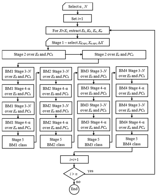
Figure 1.
Flowchart of the MFPCG.
The MFPCG Algorithm and flowchart show the MFPCG results in four qualitative assessments for the favorability of intervention R over the target population for each of the proxies, Xi, of the intervention outcome. MFPCG does not need numerous assumptions to justify its conclusion, if any. The only notable exception is the hill preference assumption that, on the one hand, is easily proven if present and, on the other hand, is a significant relaxation of the monotonic preference assumption required in DID.
4. Annuloplasty Favorability Case Study
We shall illustrate our proposed method with a case study from medical practice.
Ischemic heart disease (IHD) (also known as coronary heart disease or coronary artery disease) is among the most common heart diseases worldwide. When IHD is additionally complicated with a secondary mitral regurgitation (MR), the mitral valve (MV) between the left heart chambers (the left atrium, LA, and the left ventricle, LV) does not fully close. Blood leaks backward across the valve and into the LA to form the regurgitation volume (RV). The prognosis for patients with ischemic MR (IMR) is worse than when the MR is caused by other conditions (e.g., primary MR, which is caused by a primary abnormality of one or more components of the valve apparatus—leaflets, chordae tendineae, papillary muscles, annulus, etc.). Such patients suffer an abnormality of the myocardium of the LV of the heart that leads to the remodeling of the LV and dislocation of the papillary muscles. This complex mechanism is the leading cause of IMR, which deteriorates over time and can cause various levels of heart failure [41,42,43]. Patients with mild IMR (also called grade I) usually undergo an isolated coronary artery bypass graft (CABG). Patients with severe IMR traditionally undergo a combined operation that includes mitral valve repair (MVRepair) through annuloplasty or valve replacement, combined with a coronary artery bypass (MVRepair + CABG). These surgical recommendations are well-accepted in medical practice [44].
When patients have moderate or moderate-to-severe IMR, the optimal treatment is rigorously debated due to factors such as recurring IMR several months to several years after surgery, long-term survival rates, etc. Research in favor of the combined intervention is proposed in [45,46,47,48,49]. Research that outlined the shortcomings of anuloplasty in such patients is provided in [50,51,52]. The available studies included comparatively small groups of patients, and the results are hard to compare, as the studies used different diagnostic criteria and operation techniques. Our analysis aims to demonstrate if annuloplasty positively influences patients with moderate and moderate-to-severe IMR.
Part of the patients with IMR in our study underwent MVRepair+CABG (group A), whereas the rest underwent only CABG (group B). The choice of surgical treatment in the case of IMR is not trivial, for the reasons outlined above. The choice of an approach faces the following difficulties:
- (1)
- Traditionally, the classification of patients is based on subjective expertise. There is no specific measure of how typical a patient is to a given group.
- (2)
- The groups are not homogenous. Therefore, comparing them is complicated.
Some patients are very suitable for a given procedure; others are clearly unsuitable for this procedure, but the decision is unclear and ambiguous for the remaining patients. A previous study offered two stratification algorithms to allocate the patients in each group into two comparatively more homogenous subgroups depending on the preoperative medical status of patients: comparatively preserved status (subgroups A1 and B1) and comparatively deteriorated status (subgroups A2 and B2) [53]. This allows us to avoid comparing the groups A and B. Instead, we will compare A1 and B1 on one hand and A2 and B2 on the other. As a result, we can adequately assess the effect of the annuloplasty.
We shall demonstrate the application of MFPCG to assess the effect of the annuloplasty (R) that acts in conjunction with the base intervention of revascularization (V) over two of the continuous parameters (X1 and X2), described in Section 4.1, that characterize the condition of the target population (P) of patients with moderate and moderate-to-severe IMR subjected to a combined procedure (MVRepair + CABG). The values of each parameter X for the patients in the experimental group A are measured before and after the combined procedure. We judge the effect of the annuloplasty in comparison with the effect of the isolated procedure over the same parameter X, which now characterizes the condition of the pseudo-control population (Q) of patients with severe IMR subjected to isolated revascularization (CABG). The values of parameter X are measured before and after the isolated CABG for the patients from the pseudo-control group B.
4.1. Database
The database for this case study contains the records of 169 patients with IHD (that required revascularization) and moderate and moderate-to-severe chronic IMR. The data are presented in [16]. The study was conducted among patients from the Clinic of Cardiovascular Surgery in UH “St. Marina”, Varna (Bulgaria), who underwent surgery due to IHD complicated with MR in the period from 2007 to 2022. These patients were subjected to an MVRepair+CABG (group A) or to an isolated CABG (group B) [15]. In the study, each group was further divided into two comparatively homogenous subgroups:
- Those with a comparatively preserved medical state (A1 and B1)
- Those with a comparatively deteriorated medical state (A2 and B2).
The following parameters are measured and archived for each patient:
- 20 identifiers;
- 18 anamnesis and clinical preoperative parameters; and
- 13 three-dimensional (triple) echocardiographic parameters.
The parameters were collected as part of the patient’s anamnesis or using echocardiographic equipment GE Vivid 7 PRO (till 2017) and GE Vivid 95 (afterward) (Minneapolis, MN, USA). All patients were subjected to transthoracic echocardiogram (TTE). The 13 three-dimensional parameters are measured in three different time intervals: (1) prior to surgery, (2) soon after surgery (from 5 to 30 days after surgery), and (3) late after surgery (from 6 to 54 months after surgery). So, each three-dimensional parameter contains three values at different time points. As a result, each patient is described with a 75-dimensional record that contains the above-listed parameters.
4.2. Division into Groups with Fuzzy Degrees of Membership
The work [54] presented three (one main and two auxiliary) fuzzy algorithms, which produce the degree of membership of each patient to a specific fuzzy subgroup based on the parameters available before the surgery (which are part of the 75-dimensional record for each patient). The procedures used the age of the patients, the 18 anamnesis and clinical preoperative parameters, and the preoperative values of the 13 three-dimensional echocardiographic parameters. The resulting degrees of membership coincide with the subjectively defined ones by the medical team, which are confirmed at the end of the measurement based on all parameters. Finding the degrees of membership of each patient is a form of classification that shows much better performance than other such classifiers. This is unsurprising given that the fuzzy algorithms form a specialized classifier that relies on object-specific knowledge, whereas the others are general classifiers. The fuzzy algorithms have substantially better performance measures than their crisp counterparts. That also is to be expected, since the former use more information than the latter, which incorrectly assumes that any patient is a typical representative of its group.
The main algorithm (MA) from [54] generates a fuzzy partition of the patients into two fuzzy sets (A and B) using their degrees of membership. Due to the lack of homogeneity in those two sets, the work proposed two auxiliary algorithms. They stratify each group into two homogenous subgroups according to medical state (comparatively preserved or comparatively deteriorated) using the conditional degrees of membership to the subgroups. This way, the approach is personalized and reduces the risk of incorrect decisions. It also allows for higher precision in allocating resources for the medical treatment of patients. The work compared the results of their approach with classical approaches, including Bayesian classifiers. The advantages of the classification achieved using the fuzzy algorithms were demonstrated using four criteria, including the ability of the algorithms to discern typical patients from outliers and generate a numerical estimate of the degree of typicality of patients to the subgroups.
In our paper, we use a slightly optimized version of those fuzzy algorithms. We also adapted the fuzzy algorithms to the new patient data obtained after [54] was published.
4.3. Assessing the Effect of Annuloplasty for Patients with Severe IMR Using Fuzzy Pseudo-Control Groups
We shall demonstrate the effect of annuloplasty according to two of the most significant integral diagnostic parameters that summarize the IMR status of the patient: RF (regurgitation fraction, in %) and MR (mitral regurgitation in an 8-level scale). Both parameters are measured three times: preoperatively (when the patient is admitted to the Clinic for cardiovascular surgery), early postoperatively (7–10 days after surgery), and late postoperatively (ambulatory check-ups from 6 to 54 months after surgery).
The RF (%) is interpreted through three separate parameters: preoperative regurgitation fraction (Preop_RF), early postoperative regurgitation fraction (Early_Postop_RF), and late postoperative regurgitation fraction (Late_Postop_RF). In each of its three forms, this parameter is a continuous variable measured in % and is calculated as the regurgitation volume divided by the total ejected volume (LVEDV–LVESV) [55]:
RF = 100 × RV/(LVEDV – LVESV).
Here, LVEDV is the left ventricular end-systolic volume in mL, LVESV is the left ventricular end-diastolic volume in mL, and RV is the regurgitation volume through the MV in mL, which is the volume of blood that returns into the atrium through the mitral valve.
LVEDV and LVESV are calculated using a modified Simpson’s rule with an apical 2nd and 4th chamber position, described in [56].
RV is measured from the 4th apical position using color and CW Doppler, and the radius of the proximal isovelocity surface area (PISAr) is manually measured using a magnified image and reduced Nyquist usually to 40–45, which allows us to outline the boundaries of PISA clearly. Each of the three parameters is measured three times, as a preoperative (Preop_LVEDV, Preop_LVESV, Preop_RV), early postoperative (Early_Postop_LVEDV, Early_Postop_LVESV, Early_Postop_RVR), and late postoperative (Late_Postop_LVEDV, Late_Postop_LVESV, Late_Postop_RV) parameter. In that sense, Equation (22) is three formulae, one per each period.
According to Section 3.1, expert estimates were obtained as follows: Xopt,d = RFopt,d = 0%, Xopt,up = RFopt,up = 1%, and .
The grade of mitral regurgitation (MR) is measured by an 8-level scale: 0—lack of MR; 1—(grade 0–I) trivial MR; 2—(grade I) mild MR; 3—(grade I–II) mild-to-moderate MR; 4—(grade II) moderate MR; 5—(grade II–III) moderate-to-high MR; 6—(grade III) high MR; 7—(grade above III) severe MR. The grade of MR is presented through three parameters: preoperative grade of mitral regurgitation (Preop_MR), early postoperative grade of mitral regurgitation (Early_Postop_MR), and late postoperative grade of mitral regurgitation (Late_Postop_MR). Strictly speaking, MR is a discrete parameter, yet the large count of discretes (eight) allows for an approximation by a continuous parameter at a negligible discretization error. In this way, we illustrate the ability of MFPCG to assess the influence of the effect using a continuous parameter X, measured in an ordinal scale with five or more discretes.
According to Section 3.1, expert estimates were obtained as follows: Xopt,d = MRopt,d = 0, Xopt,up = MRopt,up = 1, and .
On the one hand, we assess the effect of annuloplasty using MFPCG for patients with a relatively preserved medical state by comparing the values of both parameters for subgroups A1 and B1. We use four fuzzy samples for RF and four fuzzy samples for MR, as Section 4.3.1 and Section 4.3.2 demonstrate. The fuzzy samples are formed using all patients with the necessary characteristics, regardless of whether those are typical or outliers.
On the other hand, we assess the same effect for patients with a relatively deteriorated medical state and compare the values of MR and RF for subgroups A2 and B2. We use four different fuzzy samples for MR and four different fuzzy samples for RF, as Section 4.3.3 and Section 4.3.4 show. The fuzzy samples were also formed using all patients with the necessary characteristics, regardless of whether those are typical or outliers.
In essence, we should apply the MFPCG four times to solve the following tasks:
- (Task 1)
- Assess the effect of annuloplasty over RF for patients with a relatively preserved medical state.
- (Task 2)
- Assess the effect of annuloplasty over MR for patients with a relatively preserved medical state.
- (Task 3)
- Assess the effect of annuloplasty over RF for patients with a relatively deteriorated medical state.
- (Task 4)
- Assess the effect of annuloplasty over MR for patients with a relatively deteriorated medical state.
We solved the four tasks at a significance level of α = 0.05. The Bootstrap simulation for each statistical test is performed with N = 2000 pseudo-realities.
We form four fuzzy samples for each of the four tasks, as described in Section 1:
- Eb is a fuzzy sample that contains the values of X and their degrees of membership to the experimental group Ai before the combined intervention.
- PCb is a fuzzy sample that contains the values of X and their degrees of membership to the pseudo-control group Bi before the isolated intervention.
- Ee is a fuzzy sample that contains the values of X and their degrees of membership to the experimental group Ai late after the combined intervention.
- PCe is a fuzzy sample that contains the values of X and their degrees of membership to the pseudo-control group Bi late after the isolated intervention.
4.3.1. Effect of Annuloplasty over RF for Patients with Relatively Preserved Medical State (Task 1)
In task 1, we use four fuzzy samples for RF, as described below.
Eb is a fuzzy sample that contains 34 values of Preop_RF and their degrees of membership to the experimental group A1:
= {(57,0.630), (63,0.900), (42,0.630), (42,0.630), (57,0.360), (64,0.810), (39,0.810), (47,0.630), (55,0.900), (65,0.630), (37,0.630), (67,0.630), (65,0.490), (62,0.630), (65,0.700), (31,0.490), (53,0.630), (64,0.630), (44,0.630), (56,0.630), (68,0.700), (43,0.900), (55,0.630), (36,0.630), (55,0.490), (55,0.900), (68,0.630), (37,0.490), (64,0.630), (56,0.490), (49,0.630), (69,0.700), (45,0.900), (56,0.700)}.
PCb is a fuzzy sample that contains 43 values of Preop_RF and their degrees of membership to the pseudo-control group B1:
= {(34,0.900), (62,0.810), (28,0.900), (38,0.900), (59,0.630), (51,0.810), (38,0.630), (39,0.900), (36,0.810), (28,0.900), (24,0.900), (59,0.630), (38,0.490), (49,0.810), (40,0.900), (59,0.630), (35,0.630), (47,0.630), (24,0.490), (48,0.810), (25,0.900), (38,0.490), (34,0.900), (32,0.900), (21,0.490), (37,0.810), (22,0.630), (26,0.900), (34,0.810), (29,0.630), (36,0.900), (36,0.630), (60,0.490), (20,0.630), (21,0.900), (32,0.900), (15,0.900), (19,0.900), (31,0.700), (41,0.700), (36,0.700), (39,0.700), (21,0.357)}.
Ee is a fuzzy sample that contains 32 values of Late_Postop_RF and their degrees of membership to the experimental group A1:
= {(0,0.630), (37,0.900), (27,0.630), (43,0.630), (0,0.360), (24,0.810), (18,0.810), (12,0.630), (0,0.900), (0,0.630), (0,0.630), (0,0.630), (0,0.630), (13,0.700), (0,0.630), (0,0.630), (0,0.630), (0,0.630), (0,0.700), (0,0.900), (17,0.630), (12,0.630), (0,0.490), (0,0.900), (0,0.630), (0,0.490), (0,0.630), (18,0.490), (0,0.630), (8,0.700), (7,0.900), (0,0.700)}.
PCe is a fuzzy sample that contains 41 values of Late_Postop_RF and their degrees of membership to the pseudo-control group B1:
= {(0,0.900), (43,0.810), (6,0.900), (13,0.900), (88,0.630), (39,0.810), (48,0.630), (12,0.900), (65,0.810), (14,0.900), (0,0.900), (48,0.490), (41,0.810), (11,0.900), (38,0.630), (12,0.630), (14,0.630), (36,0.490), (58,0.810), (27,0.900), (0,0.490), (19,0.900), (24,0.900), (65,0.490), (23,0.630), (12,0.900), (43,0.810), (10,0.630), (18,0.900), (30,0.630), (41,0.490), (23,0.630), (0,0.900), (21,0.900), (33,0.900), (12,0.900), (0,0.700), (22,0.700), (0,0.700), (24,0.700), (0,0.357)}.
Table 2 presents the numerical characteristics of the four fuzzy samples.
Table 2.
The numerical characteristics and change favorability for the RF fuzzy samples for groups A1 and B1.
First, let us assess the influence of annuloplasty on the preoperative RF values.
According to Section 3.2, from , it follows that ME is less favorable than MPC. This is indicated in column four of Table 2. From , it follows that MEDE is less favorable than MEDPC. This is indicated in column four of Table 2.
Line two of Table 3 presents the p-values for the nine Bootstrap statistical tests for the BM1 Bootstrap. According to the Stage 3 Algorithm, since , then the preoperative population distributions of RF are assumed to be statistically significantly different. Since and ME = 54% > MPC = 35.5%, then the preoperative mean in the target population A1 is assumed to be statistically significantly greater than that in the pseudo-control population B1. Since and MEDE = 55.1% > MEDPC = 35.2%, then the preoperative median of the target population A1 is assumed to be statistically significantly greater than that in the pseudo-control population B1. Since , then the preoperative variance of the target population A1 is assumed statistically indistinguishable from that in the pseudo-control population B1. Since , then the preoperative interquartile interval of the target population A1 is assumed statistically indistinguishable from that in the pseudo-control population B1.
Table 3.
The p-values of the fuzzy Bootstrap statistical tests in MFPCG for parameter RF, comparing subgroups A1 and B1.
We obtained detailed results for the other three Bootstrap Modifications. Their p-values are given in lines 4, 6, and 8 of Table 3.
Let us categorize the differences between A1 and B1 using the BM1 Bootstrap. Section 3.4 defines the values of the five input variables of the discrete categorization function (20). The preoperative differences in the means of RF in the populations A1 and B1 are CM = M−1 (the preoperative mean of RF in the target population A1 is statistically significantly less favorable than that in the pseudo-control population B1). The preoperative differences in the medians of RF in the populations A1 and B1 are CMED = MED1 (the preoperative median of RF in the target population A1 is statistically significantly less favorable than that in the pseudo-control population B1). Cond1 = T, since the distributions of RF in populations A1 and B1 are statistically significantly different, and the two characteristics of dispersion in populations A1 and B1 are not statistically different. Cond2 = T, since the distributions of RF in populations A1 and B1 are statistically significantly different, and both characteristics of dispersion in populations A1 and B1 are statistically indistinguishable. Cond3 = F, since the distributions of RF in the populations A1 and B1 are not borderline statistically significantly different.
According to the last line of Table 1, the preoperative differences in the continuous parameter RF between the two populations A1 and B1 are categorized as Ct = C−1. We can see from the same line of Table 1 that we have applied Rule 5: if one of the measures of location of RF in the target population A1 is statistically significantly less favorable than that in the pseudo-control population B1, whereas the other measure of location in the target population A1 is neither statistically significantly nor borderline statistically significantly more favorable than that in the pseudo-control population B1, then categorize in C−1.
Columns 3 to 9 on line two of Table 4 show the input variables’ values and the categorization function’s values. We obtained similar results for the remaining three Bootstrap Modifications shown in lines 4, 6, and 8 of Table 4.
Table 4.
The MFPCG diagnostics of the influence of R on a continuous parameter RF, comparing subgroups A1 and B1.
Let us now assess the influence of annuloplasty on the late postoperative RF values.
According to Section 3.2, from , it follows that ME is more favorable than MPC. This is indicated in column seven of Table 2. From , it follows that MEDE is more favorable than MEDPC. This is indicated in column seven of Table 2.
Line three of Table 3 presents the p-values for the nine Bootstrap statistical tests for the first Bootstrap Modification.
The p-values of the nine Bootstrap statistical tests for BM1 Bootstrap are given on line three of Table 3. According to Section 3.3, since , then the late postoperative population distributions of RF are assumed to be statistically significantly different. Since and ME = 7.79% < MPC = 24.2%, then the late postoperative mean of the target population A1 is assumed to be statistically significantly smaller than that in the pseudo-control population B1. Since and MEDE = 0% < MEDPC = 20.7%, then the late postoperative median of the target population A1 is assumed to be statistically significantly smaller than that in the pseudo-control population B1. Since and VARE = 12.12 < VARPC = 20.12, then the late postoperative variance of the target population A1 is assumed to be statistically significantly smaller than that in the pseudo-control population B1. Since , the late postoperative interquartile range of the target population A1 is assumed statistically indistinguishable from that in the pseudo-control population B1.
Detailed results can be obtained for the other three Bootstrap Modifications. Their p-values are in lines 5, 7, and 9 of Table 3.
Let us categorize the difference between A1 and B1 using BM1 Bootstrap. According to Section 3.4, we can define the values of the five input variables of the discrete function of categorization (20). The late postoperative differences in the means of RF in the populations A1 and B1 are CM = M+1 (the late postoperative mean of RF in the target population A1 is statistically significantly more favorable than that in the pseudo-control population B1). The late postoperative differences in the medians of RF in the populations A1 and B1 are CMED = MED+1 (the late postoperative median of RF in the target population A1 is statistically significantly more favorable than that in the pseudo-control population B1). Cond1 = F, since the variances in the populations A1 and B1 are statistically different. Cond2 = F, since the variances in the populations A1 and B1 are statistically distinguishable. Cond3 = F, since the distributions of RF in the populations A1 and B1 are not borderline statistically significantly discernible.
According to the first line of Table 1, the late postoperative differences in the continuous parameter RF between the populations A1 and B1 are categorized as Ct = C+1. The same line in Table 1 shows that we have applied Rule 1: if one of the measures of location of RF in the target population A1 is statistically significantly more favorable than that in the pseudo-control population B1, whereas the other measure of location in the target population A1 is neither statistically significantly nor borderline statistically significantly less favorable than that in the pseudo-control population B1, then categorize in C+1.
Columns 3 to 9 on line three of Table 4 show the input variables’ values and the categorization function’s values. We obtained similar results for the remaining three Bootstrap Modifications, shown in lines 5, 7, and 9 of Table 4.
According to Section 3.5, the result from MFPCG for BM1 Bootstrap is (Cb, Ce) = (C−1, C+1). That result is in line two of column 10 of Table 4. Hence, b = −1, and e = 1. According to Equation (21), the result (Cb, Ce) is classified in class ’YES+’ since b − e = (−1) − 1 = −2 < −1/2. The resulting class shows that according to BM1 Bootstrap, the influence of annuloplasty has a statistically significantly favorable influence over parameter RF in populations A1 and B1. This is indicated in line two of the last column of Table 4.
Similar results can be obtained for the other three Bootstrap Modifications. The results are in lines 4, 6, and 8 of Table 4.
4.3.2. Effect of Annuloplasty over MR for Patients with Relatively Preserved Medical State (Task 2)
In task 2, we use four fuzzy samples for MR, as described below.
Eb is a fuzzy sample that contains 34 values of Preop_MR and their degrees of membership to the experimental group A1:
= {(5,0.630), (6,0.900), (4,0.630), (6,0.630), (4,0.360), (6,0.810), (5,0.810), (4,0.630), (6,0.900), (6,0.630), (4,0.630), (5,0.630), (5,0.490), (5,0.630), (6,0.700), (4,0.490), (4,0.630), (6,0.630), (5,0.630), (5,0.630), (6,0.700), (6,0.900), (6,0.630), (4,0.630), (4,0.490), (6,0.900), (4,0.630), (5,0.490), (5,0.630), (5,0.490), (5,0.630), (7,0.700), (6,0.900), (6,0.700)}.
PCb is a fuzzy sample that contains 43 values of Preop_MR and their degrees of membership to the pseudo-control group B1:
= {(3,0.900), (3,0.810), (3,0.900), (3,0.900), (4,0.630), (4,0.810), (4,0.630), (3,0.900), (4,0.810), (3,0.900), (3,0.900), (4,0.630), (4,0.490), (4,0.810), (3,0.900), (4,0.630), (4,0.630), (4,0.630), (4,0.490), (4,0.810), (3,0.900), (4,0.490), (3,0.900), (3,0.900), (4,0.490), (4,0.810), (4,0.630), (3,0.900), (4,0.810), (4,0.630), (3,0.900), (4,0.630), (4,0.490), (4,0.630), (3,0.900), (3,0.900), (3,0.900), (3,0.900), (3,0.700), (3,0.700), (4,0.700), (4,0.700), (4,0.357)}.
Ee is a fuzzy sample that contains 32 values of Late_Postop_MR and their degrees of membership to the experimental group A1:
= {(0,0.630), (2,0.900), (2,0.630), (4,0.630), (2,0.360), (4,0.810), (2,0.810), (2,0.630), (0,0.900), (0,0.630), (1,0.630), (0,0.630), (0,0.630), (1,0.700), (0,0.630), (0,0.630), (0,0.630), (0,0.630), (0,0.700), (0,0.900), (2,0.630), (2,0.630), (0,0.490), (0,0.900), (0,0.630), (0,0.490), (0,0.630), (2,0.490), (0,0.630), (1,0.700), (1,0.900), (0,0.700}.
PCe is a fuzzy sample that contains 41 values of Late_Postop_MR and their degrees of membership to the pseudo-control group B1:
= {(2,0.900), (2,0.810), (2,0.900), (2,0.900), (5,0.630), (4,0.810), (4,0.630), (2,0.900), (6,0.810), (1,0.900), (1,0.900), (3,0.490), (2,0.810), (2,0.900), (4,0.630), (1,0.630), (2,0.630), (4,0.490), (4,0.810), (4,0.900), (1,0.490), (1,0.900), (2,0.900), (5,0.490), (4,0.630), (2,0.900), (4,0.810), (2,0.630), (2,0.900), (2,0.630), (4,0.490), (3,0.630), (0,0.900), (2,0.900), (4,0.900), (2,0.900), (0,0.700), (1,0.700), (0,0.700), (2,0.700), (0,0.357)}.
The numerical realization of MFPCG for task 2 is given in Table 5, Table 6 and Table 7, which have a similar structure to Table 2, Table 3 and Table 4 described in Section 4.3.1.
Table 5.
The numerical characteristics and change favorability for the MR fuzzy samples for groups A1 and B1.
Table 6.
The p-values of the fuzzy Bootstrap statistical tests in MFPCG for parameter MR, comparing subgroups A1 and B1.
Table 7.
The MFPCG diagnostics of the influence of R on a continuous parameter MR, comparing subgroups A1 and B1.
4.3.3. Effect of Annuloplasty over RF for Patients with Relatively Deteriorated Medical State (Task 3)
In task 3, we use four fuzzy samples for RF, as described below.
Eb is a fuzzy sample that contains 53 values of Preop_RF and their degrees of membership to the experimental group A2:
= {(66,0.306), (46,0.630), (68,0.700), (65,0.900), (71,0.490), (61,0.700), (58,0.810), (50,0.810), (64,0.490), (50,0.306), (47,0.900), (53,0.900), (41,0.630), (51,0.306), (70,0.900), (65,0.700), (54,0.700), (33,0.810), (66,0.810), (71,0.490), (60,0.630), (54,0.810), (61,0.490), (50,0.490), (34,0.630), (63,0.700), (69,0.700), (63,0.900), (38,0.900), (64,0.700), (71,0.630), (60,0.700), (63,0.490), (73,0.700), (68,0.700), (43,0.700), (43,0.810), (59,0.700), (59,0.900), (65,0.490), (74,0.900), (50,0.700), (73,0.700), (82,0.700), (70,0.900), (50,0.900), (76,0.700), (51,0.630), (77,0.900), (43,0.900), (63,0.700), (68,0.630), (48,0.630)}.
PCb is a fuzzy sample that contains 39 values of Preop_RF and their degrees of membership to the pseudo-control group B2:
= {(50,0.490), (49,0.490), (46,0.357), (38,0.260), (31,0.630), (35,0.490), (26,0.700), (21,0.700), (31,1.000), (48,0.490), (28,0.630), (24,1.000), (43,0.510), (39,0.630), (24,0.490), (46,0.630), (50,0.357), (55,0.630), (39,0.700), (54,1.000), (47,1.000), (50,0.700), (56,0.810), (30,0.490), (47,1.000), (30,0.700), (41,0.700), (57,1.000), (60,1.000), (48,0.490), (45,0.357), (35,0.260), (44,0.630), (30,0.510), (43,0.260), (40,0.357), (53,1.000), (23,1.000), (74,1.000)}.
Ee is a fuzzy sample that contains 44 values of Late_Postop_RF and their degrees of membership to the experimental group A2:
= {(0,0.700), (42,0.900), (0,0.490), (0,0.700), (0,0.810), (0,0.810), (14,0.490), (31,0.306), (20,0.900), (11,0.700), (0,0.810), (10,0.490), (0,0.630), (21,0.810), (10,0.490), (0,0.490), (0,0.630), (0,0.700), (20,0.700), (7,0.900), (13,0.900), (0,0.700), (12,0.700), (18,0.490), (24,0.700), (0,0.700), (0,0.700), (19,0.810), (0,0.700), (29,0.900), (0,0.490), (0,0.900), (0,0.700), (25,0.700), (0,0.700), (0,0.900), (0,0.900), (6,0.700), (0,0.630), (0,0.900), (11,0.900), (0,0.700), (0,0.630), (0,0.630)}.
PCe is a fuzzy sample that contains 32 values of Late_Postop_RF and their degrees of membership to the pseudo-control group B2:
= {(43,0.490), (35,0.490), (53,0.630), (0,0.700), (0,0.700), (7,1.000), (21,0.490), (15,1.000), (11,0.510), (44,0.630), (25,0.490), (78,0.630), (0,0.357), (77,0.630), (70,1.000), (57,1.000), (11,0.700), (66,0.490), (28,1.000), (0,0.700), (48,0.700), (76,1.000), (45,0.490), (19,0.357), (23,0.260), (10,0.630), (13,0.510), (32,0.260), (29,0.357), (16,1.000), (15,1.000), (47,1.000)}.
Table 8, Table 9 and Table 10 provide the numerical realization of MFPCG for task 3. These tables have a similar structure to Table 2, Table 3 and Table 4 described in Section 4.3.1.
Table 8.
The numerical characteristics and change favorability for the RF fuzzy samples for groups A2 and B2.
Table 9.
The p-values of the fuzzy Bootstrap statistical tests in MFPCG for parameter RF, comparing subgroups A2 and B2.
Table 10.
The MFPCG diagnostics of the influence of R on a continuous parameter RF, comparing subgroups A2 and B2.
4.3.4. Effect of Annuloplasty over MR for Patients with Relatively Deteriorated Medical State (Task 4)
In task 4, we use four fuzzy samples for MR, as described below.
Eb is a fuzzy sample that contains 53 values of Preop_MR and their degrees of membership to the experimental group A2:
= {(5,0.306), (5,0.630), (6,0.700), (6,0.900), (4,0.490), (6,0.700), (6,0.810), (6,0.810), (6,0.490), (4,0.306), (5,0.900), (6,0.900), (4,0.630), (4,0.306), (6,0.900), (6,0.700), (5,0.700), (4,0.810), (5,0.810), (5,0.490), (4,0.630), (6,0.810), (5,0.490), (5,0.490), (4,0.630), (6,0.700), (6,0.700), (6,0.900), (6,0.900), (6,0.700), (5,0.630), (6,0.700), (6,0.490), (6,0.700), (6,0.700), (6,0.700), (5,0.810), (5,0.700), (6,0.900), (5,0.490), (7,0.900), (7,0.700), (7,0.700), (7,0.700), (6,0.900), (6,0.900), (6,0.700), (6,0.630), (7,0.900), (6,0.900), (6,0.700), (6,0.630), (6,0.630)}
PCb is a fuzzy sample that contains 38 values of Preop_MR and their degrees of membership to the pseudo-control group B2:
= {(4,0.490), (4,0.490), (3,0.260), (4,0.630), (4,0.490), (3,0.700), (3,0.700), (4,1.000), (4,0.490), (4,0.630), (4,1.000), (4,0.510), (4,0.630), (4,0.490), (4,0.630), (4,0.357), (4,0.630), (3,0.700), (4,1.000), (4,1.000), (3,0.700), (4,0.810), (4,0.490), (4,1.000), (3,0.700), (3,0.700), (4,1.000), (3,1.000), (4,0.490), (3,0.357), (3,0.260), (4,0.630), (4,0.510), (4,0.260), (4,0.357), (5,1.000), (4,1.000), (7,1.000)}.
Ee is a fuzzy sample that contains 44 values of Late_Postop_MR and their degrees of membership to the experimental group A2:
= {(0,0.700), (5,0.900), (0,0.490), (2,0.700), (0,0.810), (0,0.810), (2,0.490), (2,0.306), (2,0.900), (1,0.700), (0,0.810), (2,0.490), (0,0.630), (1,0.810), (1,0.490), (0,0.490), (0,0.630), (0,0.700), (2,0.700), (2,0.900), (1,0.900), (0,0.700), (2,0.700), (2,0.490), (2,0.700), (0,0.700), (0,0.700), (1,0.810), (0,0.700), (2,0.900), (0,0.490), (0,0.900), (0,0.700), (2,0.700), (0,0.700), (0,0.900), (0,0.900), (1,0.700), (0,0.630), (0,0.900), (1,0.900), (0,0.700), (0,0.630), (0,0.630)}.
PCe is a fuzzy sample that contains 32 values of Late_Postop_MR and their degrees of membership to the pseudo-control group B2:
= {(4,0.490), (4,0.490), (5,0.630), (1,0.700), (0,0.700), (2,1.000), (2,0.490), (2,1.000), (2,0.510), (4,0.630), (3,0.490), (4,0.630), (2,0.357), (5,0.630), (4,1.000), (4,1.000), (2,0.700), (5,0.490), (4,1.000), (0,0.700), (4,0.700), (4,1.000), (5,0.490), (2,0.357), (2,0.260), (1,0.630), (1,0.510), (2,0.260), (2,0.357), (2,1.000), (2,1.000), (5,1.000)}.
The numerical realization of MFPCG for task 4 is given in Table 11, Table 12 and Table 13, which have a similar structure to Table 2, Table 3 and Table 4 described in Section 4.3.1.
Table 11.
The numerical characteristics and change favorability for the MR fuzzy samples for groups A2 and B2.
Table 12.
The p-values of the fuzzy Bootstrap statistical tests in MFPCG for parameter MR, comparing subgroups A2 and B2.
Table 13.
The MFPCG diagnostics of the influence of R on a continuous parameter MR, comparing subgroups A2 and B2.
4.4. Summary
In the annuloplasty favorability case study, the MFPCG Algorithm (Section 3.6) was applied two times. Let U be the super-population of patients diagnosed with IHD and moderate and moderate-to-severe IMR with indications for surgery. In both applications, X1 = RF and X2 = MR. In the first application, P is the population from U consisting of patients with indications for combined surgery who have a relatively preserved medical state (subgroup A1 comprises patients from P); Q is the population of U consisting of patients with indications for an isolated intervention who have a relatively preserved medical state (subgroup B1 comprises patients from Q). In the second application, P is the population of U consisting of patients with indications for combined surgery who have a relatively deteriorated medical state (subgroup A2 comprises patients from P); Q is the population of U consisting of patients with indications for an isolated intervention who have relatively deteriorated medical state (subgroup B2 comprises patients from Q).
5. Validation of the Case Study Conclusions
5.1. External Validation
Each of the four tasks formulated in Section 3 is solved four times depending on the modification of the Bootstrap tests performed.
Table 4, Table 7, Table 10 and Table 13 show that for each of the sixteen solutions, we obtain the following MFPCG result: (Cb, Ce) = (–1, +1), with the MFPCG category: ‘YES+’, as described in Section 3.5. In their entirety, the results show a favorable effect of annuloplasty on the analyzed parameters, both for patients with a relatively preserved medical state and patients with a relatively deteriorated medical state.
These conclusions are in accordance with the conclusions in [15,57,58,59], which is an external validation of the MFPCG results for annuloplasty favorability. This affirmative result is an improvement over the aforementioned publications in the following ways:
- In this study, we used data for all available patients, whereas the cited sources analyzed the data after rejecting outliers (which comprised about 20% of the data).
- In our study, we prove every influence using four different Bootstrap Modifications, improving the conclusions’ statistical credibility. Our approach uses a cluster of tests instead of individual p-values, which is in accordance with the modern trends in data analysis [33,39].
- Here, we discuss the typicality of patients to a respective subgroup for the first time, whereas in earlier works, the classification is considered absolute (crisp).
- The statistical support for a favorable effect of annuloplasty is efficiently completed using only two integral parameters. In contrast, the earlier works used a double-digit count of parameters to reach the same conclusions.
5.2. Fuzzy DID Method (FDID)
For the sake of internal validation, we will compare the acquired conclusions on the annuloplasty favorability with the results of the DID method. To improve the comparability of DID and MFFCG results, we developed a fuzzy DID that uses Bootstrap in the four discussed modifications to estimate the confidence interval (CI) of the average treatment effect (ATE):
FDID Algorithm
- Select the significance level, α, and the number of pseudo-realities, N, to construct the Bootstrap CIs.
- Set i = 1.
- Choose X = Xi.
- Extract from the database the fuzzy samples Eb, PCb, Ee, and PCe for this X.
- Estimate the fuzzy mean values of the four samples ME,b, MPC,b, ME,e, and MPC,e using (8).
- Estimate the fuzzy DID estimator as the ATE:
ATE = (ME,e − MPC,e) − (ME,b − MPC,b)
- 7.
- Find the index of the empirical α/2-quantile from the Bootstrap distribution of ATE, as Nd = round(N × α/2).
- 8.
- Find the index of the empirical (1–α/2)-quantile from the Bootstrap distribution of ATE, as Nu = round(N − N × α/2).
- 9.
- Repeat for Bootstrap Modification BMk (k = 1, 2, 3, 4):
- 9.1.
- Repeat for pseudo-reality r (r = 1, 2, …, N):
- 9.1.1.
- From sample Eb, generate sEb,r, using Bootstrap Modification BMk.
- 9.1.2.
- From sample PCb, generate sPCb,r, using Bootstrap Modification BMk.
- 9.1.3.
- From sample Ee, generate sEe,r, using Bootstrap Modification BMk.
- 9.1.4.
- From sample PCe, generate sPCe,r, using Bootstrap Modification BMk.
- 9.1.5.
- Estimate the fuzzy mean values of the four synthetic samples sME,b,r, sMPC,b,r, sME,e,r, and sMPC,e,r using (8).
- 9.1.6.
- Estimate the fuzzy DID estimator as sATEr in the r-th pseudo-reality:sATEr = (sME,e,r − sMPC,e,r) − (sME,b,r − sMPC,b,r)
- 9.2.
- Sort the synthetic sATEr in ascending order and obtain sATEsort,r (r = 1, 2, …, N).
- 9.3.
- Estimate the Reverse Percentile 100 × (1 – α)%-CI for ATE using Bootstrap Modification BMk:Pr{2 × ATE – sATEsort,Nu < ATE < 2 × ATE – sATEsort,Nd} = 1 – α
- 10.
- Set i = i+1.
- 11.
- If i < n, then go to step 3. Otherwise, end the algorithm.
5.3. Case Study Solved with FDID
In essence, we should apply the FDID four times to solve the four tasks formulated in Section 4.3. For the sake of comparability, we solved the four tasks at a significance level of α = 0.05, and the Bootstrap CIs were calculated with N = 2000 pseudo-realities.
5.3.1. FDID Solution of Task 1 (Effect of Annuloplasty over RF for A1 and B1 Patients)
First, we will solve task 1, as described in Section 4.3, using the fuzzy DID method. We shall use the four samples given in Section 4.3.1. Table 14 shows the fuzzy mean values of the four samples. The ATE for task 1 is (–43.9%), given on line 4, column 4 of the table. Those results are illustrated in Figure 2, which shows the three temporal functions of the fuzzy means in A1, B1, and the counterfactual of A1, along with ATE. After applying the algorithm of the fuzzy DID, we obtained four Reverse Percentile 95%-CIs for ATE in task 1:
Table 14.
Fuzzy means of RF, % for subgroups A1 and B1.
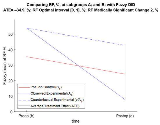
Figure 2.
DID graphical illustration for task 1.
- For BM1, Pr{−43.7 < ATE < −26.1} = 0.95;
- For BM2, Pr{−44.6 < ATE < −27.1} = 0.95;
- For BM3, Pr{−44.1 < ATE < −26} = 0.95;
- For BM4, Pr{−44.4 < ATE < −26.9} = 0.95.
5.3.2. FDID Solution of Task 2 (Effect of Annuloplasty over MR for A1 and B1 Patients)
We shall use the four samples given in Section 4.3.2. Table 15 shows the fuzzy mean values of the four samples. The ATE for task 2 is (–3.31%), given on line 4, column 4 of the table. Those results are illustrated in Figure 3, which shows the three temporal functions of the fuzzy means in A1, B1, and the counterfactual of A1, along with ATE. After applying the algorithm of the fuzzy DID, we obtained four Reverse Percentile 95%-CIs for ATE in task 2:
Table 15.
Fuzzy means of MR, % for subgroups A1 and B1.
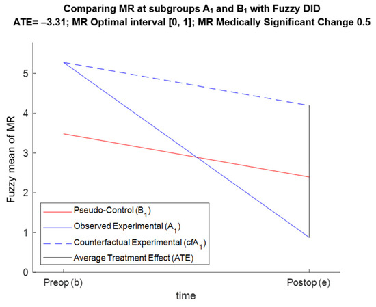
Figure 3.
DID graphical illustration for task 2.
- For BM1, Pr{−3.97 < ATE < −2.67} = 0.95;
- For BM2, Pr{−3.91 < ATE < −2.54} = 0.95;
- For BM3, Pr{−4 < ATE < −2.64} = 0.95 = 0.95;
- For BM4, Pr{−3.9 < ATE < −2.54} = 0.95 = 0.95.
5.3.3. FDID Solution of Task 3 (Effect of Annuloplasty over RF for A2 and B2 Patients)
We shall use the four samples given in Section 4.3.3. Table 16 shows the fuzzy mean values of the four samples. The ATE for task 3 is (–41.4%), given on line 4, column 4 of the table. Those results are illustrated in Figure 4, which shows the three temporal functions of the fuzzy means in A2, B2, and the counterfactual of A2, along with ATE. After applying the algorithm of the fuzzy DID, we obtained four Reverse Percentile 95%-CIs for ATE in task 3:
Table 16.
Fuzzy means of RF, % for subgroups A2 and B2.
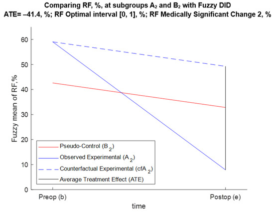
Figure 4.
DID graphical illustration for task 3.
- For BM1, Pr{−52.5 < ATE < −29.5} = 0.95;
- For BM2, Pr{−54.5 < ATE < −29.7} = 0.95;
- For BM3, Pr{−52.7 < ATE < −30.5} = 0.95;
- For BM4, Pr{−54 < ATE < −29.9} = 0.95.
5.3.4. FDID Solution of Task 4 (Effect of Annuloplasty over MR for A2 and B2 Patients)
We shall use the four samples given in Section 4.3.4. Table 17 shows the fuzzy mean values of the four samples. The ATE for task 4 is (−3.87%), given on line 4, column 4 of the table. Those results are illustrated in Figure 5, which shows the three temporal functions of the fuzzy means in A2, B2, and the counterfactual of A2, along with ATE. After applying the algorithm of the fuzzy DID, we obtained four Reverse Percentile 95%-CIs for ATE in task 4:
Table 17.
Fuzzy means of MR, % for subgroups A2 and B2.
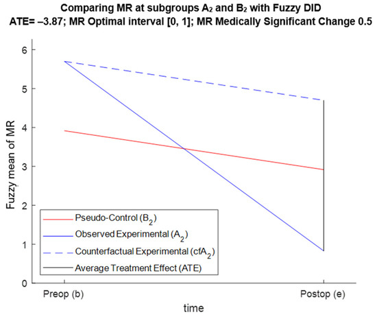
Figure 5.
DID graphical illustration for task 4.
- For BM1, Pr{−4.62 < ATE < −3.17} = 0.95;
- For BM2, Pr{−4.56 < ATE < −3.1} = 0.95;
- For BM3, Pr{−4.63 < ATE < −3.15} = 0.95;
- For BM4, Pr{−4.62 < ATE < −3.09} = 0.95.
5.4. Internal Validation with FDID
According to Section 5.3, each of the four tasks was solved four times depending on the Bootstrap Modification used to construct the CIs of ATE. For each of the 16 solutions, we obtain an ATE that is statistically significant and practically favorable. This shows the favorable effect of annuloplasty on the analyzed parameters for both subgroups A1 and B1, and subgroups A2 and B2.
The conclusions from FDID are in accordance with the conclusions from MFPCG from Section 5.1, which internally validate the results of MFPCG. The affirmative result of MFPCG relates to the affirmative result of FDID in the following ways:
- The results from FDID are conditional upon the assumptions of the method. We do not have a way of proving the parallel trend assumption, as shown in Figure 2, Figure 3, Figure 4 and Figure 5. We also cannot prove that, in this particular case, the classical normal linear regression model (CNLRM) assumptions [9,60] about nullity, homoskedasticity, normality, correlation, multicollinearity, and linearity hold.
- Both methods use data for all available patients without rejecting outliers.
- Both methods use a cluster of tests instead of individual p-values.
- Both methods consider the typicality of patients to a respective subgroup.
- MFPCG produces qualitative results that annuloplasty is favorable for patients with an average or average-to-severe IMR. At the same time, the FDID produced quantitative results as to how much the annuloplasty improved the outcome for those patients compared with patients with isolated CABG.
5.5. Internal Validation with Fuzzy RDD (FRDD)
For the sake of internal validation, we also compared the acquired conclusions on the annuloplasty favorability with the results of the RDD method. To improve the comparability of RDD and MFFCG results, we developed a fuzzy RDD (FRDD) that uses Bootstrap in the four discussed modifications, on the one hand, to estimate the CIs of ATE, and on the other hand, to identify whether the reduced Eb and PCb have statistically indistinguishable Xi values. There is no obvious scalar discriminant variable that separates the experimental and the control groups. The main challenge was that, in our example, the assignment to the experimental or control groups was performed by the main algorithm from [54]. MA produces a degree of membership to the combined-operation group (μA) and to the isolated-procedure group (μB = 1 – μA) for each patient. The closer μA and μB are, the nearer the patient is to the hypothetical cutoff surface of the vector discriminant variable. So, we estimated that the reduced fuzzy samples rEb, and rEe are derived from Eb and Ee by purging all patients with μA > μcutoff (for some pre-selected values of μcutoff). Similarly, the reduced fuzzy samples rPCb and rPCe are derived from PCb and PCe by purging all patients with μB > μcutoff. If at least one of the four reduced samples has a cardinality less than six, or its sum of degrees of membership is less than 3, then we consider that the restriction is too strict for any additional data processing, and the method does not produce a result. If not, then using the four Bootstrap Modifications, we can test whether rEb and rPCb are statistically different. If they are not, then the method does not produce a result. However, if Eb is statistically indistinguishable from PCb, then we can unite the two samples into the fuzzy sample Ub and estimate its fuzzy mean value, MU,b, using (8). In that case, we can safely assume that the fuzzy mean values of rEb and rPCb are equal and coincide with the fuzzy mean value of Ub:
MrE,b = MrPC,e = MU,b
Then, the fuzzy RDD estimator of the outcome is the reduced ATE (rATE):
rATE = (MrE,e − MrPC,e)
Here, FRDD acts almost the same as RCT, since the reduced pseudo-control group is indistinguishable from the experimental group, and we can at least mentally assume a random partition of the patients. Formula (27) is a special case of the (25) under the assumption (26). We will finish the FRDD Algorithm by calculating the four Reverse Percentile 100 × (1 – α)%-CI for rATE using Bootstrap Modification BMk with the method described in the FDID Algorithm.
We have not provided the FRDD Algorithm in this paper, since its application turned out to be unsuccessful. For μcutoff = 0.7, the cardinality of the reduced samples was between 8 and 18 for all four tasks. That was enough to compare rEb and rPCb. However, for tasks 2, 3, and 4, the 20 most important tests (4 for identity of distributions, 8 for equality of fuzzy means, and 8 for equality of fuzzy medians) all have p-values of zero. For task 1, there was a mixed bag of results—the eight tests for equality of fuzzy means had p-values less than α, the eight tests for equality of fuzzy medians showed borderline statistical significance, and only one of the tests for identity of distributions showed statistical significance. Overall, there is sufficient evidence that, for task 1, rEb and rPCb are different. Thus, the entire algorithm failed.
For μcutoff = 0.69, the cardinality of the reduced samples was between 1 and 4 for all four tasks. Since the cardinality was less than 6, the FRDD failed again.
The failure of FRDD to solve any of the four tasks in the annuloplasty favorability case study was expected due to the limitations of RDD, discussed in Section 1.
6. Discussion and Conclusions
6.1. Basic Idea and Adaptability of MFPCG
The MFPCG Algorithm may seem complicated to practitioners. Yet, it reflects a simple idea—in the absence of a control group, it is sometimes possible to prove a statistical influence of R with a pseudo-control group using a certain parameter X. For example, R has a favorable influence over X if there is a statistically significantly less favorable value in the experimental group before R, and more favorable values after R, in comparison to the pseudo-control group. Then, the differences between the control and pseudo-control groups are irrelevant to the statistical conclusions. The latter cannot be rejected by showing that the pseudo-control group is different from the experimental group. For that reason, the method has the potential to be of use.
However, such conclusions are not always possible, e.g., before and after intervention R, X is less favorable in the experimental group than in the pseudo-control group.
MFPCG has considerable adaptability (and even parametrization in future developments). The version we proposed in this paper should only be interpreted as general guidance. It is sufficient only to follow the key ideas and philosophy of the approach. Every time the method is applied, it is likely that some steps ought to be modified to adjust to that specific problem and its need for classification. Therefore, the method’s applicability is broader than our discussion could allude to. The values proposed in Section 3 are robust, yet every practitioner can modify them to fit their specific task. Future researchers can even adapt the name of the method, since some fuzzy purists would have issues with our interpretation of fuzziness, in line with the discussion in Section 2 on that matter. We are perfectly happy if researchers call our novel approach the Method of the Weighted Pseudo-Control Group (MWPCG).
Stage 4 of MFPCG summarizes the results from stages 2 and 3. It has the highest potential to adapt to the specific problem by modifying the proposed rules and/or formulating new ones. This also refers to how stage 4 is formalized. In Section 3.4, we presented two approaches to suit people with different propensities to formalization. The rule-based approach is relatively compact. The function-based approach achieves the same categorization of the differences between populations with less effort and required attention from the practitioner. Both approaches are algorithmically equivalent. However, choosing one over the other is a prerogative of the practitioner applying the method. We can also develop a third approach, where the inputs are all possible combinations of the five input parameters from Section 3.4. We can develop a table similar to Table 2, with columns CM, CMED, Cond1, Cond2, Cond3, Ct, and Rule. That table should have 7 × 7 × 2 × 2 × 2 = 319 rows (note that Table 2 is a compact version of that 319-row table). Performing stage 4 of MFPCG with that extended table can be called the explicit function-based approach. The user’s preference shall dictate which approach would be used. The descending order of the three approaches regarding compactness is: 1- the rule-based, 2- the function-based, and 3- the explicit function-based. However, that order coincides with the ascending order of logical simplicity. Therefore, the choice of approach depends on the user’s trade-off between compact presentation and logical complexity.
From the flowchart in Figure 1 and the MFPCG Algorithm, we can see that our novel method can be adapted for parallel computing. The Stage 2 blocks can be calculated independently. The same applies to the four BMk meta-blocks (each including two Stage-3 blocks, two Stage-4 blocks, and one Stage-5 block). The whole section in the flowchart regarding Xi can be calculated as n independent parallel processes. The most time-consuming parts of the discussed algorithm are the eight Stage-3 blocks. In each of them, we calculate nine statistical tests. Each one of those blocks can be calculated as five independent parallel processes (it is not computationally efficient to separate a one-tailed statistical test from its two-tailed counterpart). Finally, each of those five independent parallel processes can be separated into N subprocesses estimating the individual independent pseudo-realities. It thus follows that the sky is the limit as far as parallel computing is concerned. As a result, we claim that the MFPCG can solve big-data problems.
6.2. Limitations of MFPCG
The first limitation of MFPCG is that, in its current form, it cannot deal with valley preferences as defined in [40]. The method would need to undergo significant restructuring to adapt to such preferences. However, if the preferences are multi-modal, no major adaptation would help. Luckily, such preferences are very rare in medical studies.
A second limitation is that sometimes MFPCG cannot assess the favourability of the intervention. MFPCG works by comparing the qualitative differences between the experimental and the control groups before and after the intervention. For example, if before and after intervention R, X is more favorable in the experimental group than in the pseudo-control group, then no conclusion can be reached regardless of the relative magnitude of this favourability.
Another major limitation of MFPCG transpires in the case where a significant factor changes in the experimental group differently from the way it changes in the pseudo-control group. For example, such a situation would arise if the medical team focused its efforts on patients with base intervention V and investigated intervention R more than on those with only V intervention. This can occur due to financial considerations or due to cognitive biases. Mathematically, this is a likely problem and causes concern. However, such cases are rare in medical research that is free from fraudulent or unethical activities. This limitation is an Achilles heel for any quasi-experiment designs and is not unique to MFPCG.
6.3. Synergies of MFPCG, FRDD, and FDID
It should be clear by now that MFPCG, FRDD, and FDID are all making causal inferences between the intervention R and the outcome. However, the three methods considerably differ:
- FDID always produces a quantitative assessment of the influence, and FRDD sometimes produces a quantitative assessment of the influence, whereas MFPCG sometimes produces a qualitative assessment of that influence.
- FRDD and FDID apply only to monotonic preferences over X, whereas MFPCG deals with hill preferences that are very applicable in medical studies, especially in the current age of overmedication in Western societies.
- FDID uses many assumptions that are hard to verify (the same is true to a smaller extent about FRDD), unlike MFPCG.
- FRDD and FDID only deal with mean values, whereas the more complex MFPCG operates on distributions, means, medians, standard deviations, and interquartile ranges.
- FRDD and FDID are incapable of assessing the practical significance of observed changes regardless of their statistical significance, whereas this aspect is incorporated in MFPCG.
- FRDD and FDID are easy to implement, whereas MFPCG is computationally challenging.
- There is considerable knowledge of how to implement and modify FRDD and FDID to deal with different problems since these are well known, whereas MFPCG is a new approach.
The above considerations show that MFPCG is not an alternative to FRDD or FDID but rather a complement. The three methods should be used in conjunction:
- (1)
- We should always start by applying FRDD. It generally works when there are large experimental and pseudo-control groups. The quantitative result, if any, statistically proves that the pseudo-control sample is, in fact, the control one, since there is no statistically significant difference between the pre-intervention samples. If the values of X in the fuzzy samples are in the region of monotonic preferences, the results of FRDD would be useful.
- (2)
- We then try MFPCG. If the method works, it will provide a very reliable qualitative assessment of the positive or negative influence of the intervention R.
- (3)
- We can finish with FDID. The reliability of the quantitative result depends on the validity of the assumptions of the method. If the values of X in the fuzzy samples are in the region of monotonic preferences, the results of FDID would be useful.
6.4. Applications of MFPCG
Our expectations are that the fuzzy sample input of MFPCG would facilitate its application, since it allows for encoding the uncertainty and ambiguity in the data. The latter is a modern trend in statistical data analysis. Using fuzzy samples in medical research is a well-established practice. The works [13,14] describe their successful use in medical case studies. On the other hand, MFPCG follows the trend that statistical inference should be based on a cluster of tests as opposed to one test. This approach is proposed and motivated in medical case studies in [39,61,62]. The size of the cluster of tests is quadrupled by the fuzziness of the data. As the flowchart of MFPCG shows, the influence of R over Xi is determined by 72 fuzzy statistical tests. In most cases, we will use not one but n parameters Xi. Consequently, the influence of R over parameters Xi is determined using 72n statistical tests (in the special case of crisp samples, those two values decrease to 18 and 18n, respectively). On the one hand, we can interpret the uncertainty of data in a way that enhances the comprehension of the studied effect. On the other hand, we respond to recent criticism of the single p-value concept [63].
The proposed MFPCG was invented to solve problems in medical studies. It can be applied in experimental quantitative research for solving problems from econometrics, education, statistics, public administration, social sciences, political science, sports management, etc. Of course, in those new areas, it is more likely to encounter multi-modal preferences, which could prevent us from using the method.
6.5. Future Research
Future research should focus on some MFPCG modifications while preserving its key philosophy. It is also worth testing the implementation of the method over other databases from other areas of knowledge, as the existence of control groups might be an issue in areas outside medical research.
Some of the members of the team of authors are currently developing a new method that unites FDID and FRDD, which can provide a different perspective on the problem of assessing the influence of an intervention over a target population.
Author Contributions
Conceptualization, K.T., N.N. and M.D.; methodology, K.T, S.I., N.N. and M.D.; software, K.T. and M.S.; validation, K.T., M.S., S.I. and M.D.; investigation, P.P., D.P., K.T., N.N., S.I. and M.D.; data curation, P.P. and D.P.; writing—original draft preparation, D.P., S.I., M.D. and M.S.; writing—review and editing, K.T., N.N. and D.P.; supervision, N.N. and P.P.; funding acquisition, K.T. All authors have read and agreed to the published version of the manuscript.
Funding
This research was funded by the University of Tasmania/Australian Maritime College (RT.112222).
Institutional Review Board Statement
The study was conducted in accordance with the Declaration of Helsinki, and approved by the Ethics in Research Committee of Medical University—Varna “Prof. Dr. Paraskev Stoyanov” (protocol 026-188/30 December 2021).
Informed Consent Statement
Informed consent was obtained from all subjects involved in the study.
Data Availability Statement
The original contributions presented in the study are included in the article, further inquiries can be directed to the corresponding author.
Acknowledgments
The authors would like to sincerely thank the anonymous reviewers and the academic editor who helped to substantially improve this paper.
Conflicts of Interest
The authors declare no conflicts of interest.
References
- Hinkelmann, K.; Kempthorne, O. Design and Analysis of Experiments, Volume I: Introduction to Experimental Design, 2nd ed.; Wiley Series of Probability and Statistics: Washington, DC, USA, 2008. [Google Scholar]
- Bailey, R.A. Design of Comparative Experiments; Cambridge University Press: Cambridge, UK, 2008; ISBN 978-0-521-68357-9. [Google Scholar]
- Everitt, B.S. The Cambridge Dictionary of Statistics; Cambridge University Press: Cambridge, UK, 2002; ISBN 0-521-81099-X. [Google Scholar]
- Chalmers, T.C.; Smith, H.; Blackburn, B.; Silverman, B.; Schroeder, B.; Reitman, D.; Ambroz, A. A method for assessing the quality of a randomized control trial. Control. Clin. Trials 1981, 2, 31–49. [Google Scholar] [CrossRef]
- Eddy, D.M. Evidence-based medicine: A unified approach. Health Aff. 2005, 24, 9–17. [Google Scholar] [CrossRef]
- Robson, L.S.; Shannon, H.S.; Goldenhar, L.M.; Hale, A.R. Quasi-experimental and experimental designs: More powerful evaluation designs. In Guide to Evaluating the Effectiveness of Strategies for Preventing Work Injuries; Department of Health and Human Services, National Institute for Occupational Safety and Health: Cincinnati, OH, USA, 2001; pp. 29–42. [Google Scholar]
- Kampenes, V.B.; Dybå, T.; Hannay, J.E.; Sjøberg, D.I.K. A systematic review of quasi-experiments in software engineering. Inf. Softw. Technol. 2009, 51, 71–82. [Google Scholar] [CrossRef]
- Roth, J.; Sant’Anna, P.H.C.; Bilinski, A.; Poe, J. What’s trending in difference-in-differences? A synthesis of the recent econometrics literature. J. Econom. 2023, 235, 2218–2244. [Google Scholar] [CrossRef]
- Poole, M.A.; O’Farrell, P.N. The assumptions of the linear regression model. Trans. Inst. Br. Geogr. 1971, 52, 145–158. [Google Scholar] [CrossRef]
- Ryan, A.M.; Burgess, J.F., Jr.; Dimick, J.B. Why we should not be indifferent to specification choices for difference-in-differences. Health Res. Educ. Trust. 2015, 50, 1211–1235. [Google Scholar] [CrossRef]
- Abadie, A. Semiparametric difference-in-differences estimators. Rev. Econ. Stud. 2005, 72, 1–19. [Google Scholar] [CrossRef]
- Imbens, G.; Lemieux, T.H. Regression Discontinuity Designs: A Guide to Practice. National Bureau of Economic Research Technical Working Paper 337. 2007. Available online: http://www.nber.org/papers/t0337 (accessed on 10 January 2025).
- Nikolova, N.; Rodríguez, R.M.; Symes, M.; Toneva, D.; Kolev, K.; Tenekedjiev, K. Outlier detection algorithms over fuzzy data with weighted least squares. Int. J. Fuzzy Syst. 2021, 23, 1234–1256. [Google Scholar] [CrossRef]
- Farkas, Á.Z.; Farkas, V.J.; Gubucz, I.; Szabó, L.; Bálint, K.; Tenekedjiev, K.; Nagy, A.I.; Sótonyi, P.; Hidi, L.; Nagy, Z.; et al. Neutrophil extracellular traps in thrombi retrieved during interventional treatment of ischemic arterial diseases. Thromb. Res. 2019, 175, 46–52. [Google Scholar] [CrossRef]
- Mihaylova, N. Bootstrap-Based Simulation Platform for Analysis of Medical Information. Ph.D. Thesis, Nikola Vaptsarov Naval Academy, Varna, Bulgaria, 2015. [Google Scholar]
- Panayotova, D. Application of echocardiographic methods for fuzzy stratification determining the volume of surgery in patients with ischemic mitral regurgitation. In Medical Academic Repository; Medical University: Varna, Bulgaria, 2023; Available online: https://repository.mu-varna.bg/handle/nls/3461 (accessed on 23 December 2024).
- Faugeras, O.P. Maximal coupling of empirical copulas for discrete vectors. J. Multivar. Anal. 2015, 137, 179–186. [Google Scholar] [CrossRef]
- Tenekedjiev, K.; Dimitrakiev, D.; Nikolova, N. Building frequentist distributions of continuous random variables. Mach. Mech. 2002, 47, 164–168. [Google Scholar]
- Gao, S.; Zhong, Y.; Gu, C. Random weighting estimation of confidence intervals for quantiles. Aust. N. Z. J. Stat. 2013, 55, 43–53. [Google Scholar] [CrossRef]
- Poe, G.; Giraud, K.; Loomis, J. Computational methods for measuring the difference of empirical distributions. Am. J. Agric. Econ. 2005, 87, 353–365. [Google Scholar] [CrossRef]
- Wasserman, L. The Bootstrap and the Jackknife. In All of Nonparametric Statistics; Springer Texts in Statistics; Springer: New York, NY, USA, 2006; pp. 27–41. [Google Scholar] [CrossRef]
- Henderson, R. The Bootstrap: A technique for data-driven statistics. Using computer-intensive analyses to explore experimental data. Clin. Chim. Acta 2005, 359, 1–26. [Google Scholar] [CrossRef]
- González-Rodríguez, G.; Montenegro, M.; Colubi, A.; Gil, M.-A. Bootstrap techniques and fuzzy random variables: Synergy in hypothesis testing with fuzzy data. Fuzzy Sets Syst. 2006, 157, 2608–2613. [Google Scholar] [CrossRef]
- Politis, D. Computer-intensive methods in statistical analysis. Signal Process. Mag. 1998, 15, 39–55. [Google Scholar] [CrossRef]
- Chernobai, A.; Rachev, S.T.; Fabozzi, F.J. Composite goodness-of-fit tests for left-truncated loss samples. In Handbook of Financial Econometrics and Statistics; Lee, C.F., Lee, J., Eds.; Springer: New York, NY, USA, 2015; pp. 575–596. [Google Scholar] [CrossRef]
- Groebner, D.F.; Shannon, P.W.; Fry, P.C. Business Statistics—A Decision-Making Approach, 10th ed.; Pearson: London, UK, 2018; pp. 387–434. [Google Scholar]
- Böhm, W.; Hornik, K. A Kolmogorov-Smirnov test for r samples. Res. Rep. Ser. Dep. Stat. Math. 2010, 105, 103–125. [Google Scholar] [CrossRef]
- Lemeshko, B.; Gobrunova, A.A. Application and power of the nonparametric Kuiper, Watson, and Zhang tests of goodness-of-fit. Meas. Tech. 2013, 56, 465–475. [Google Scholar] [CrossRef]
- Press, W.H.; Teukolsky, S.A.; Vetterling, W.T.; Flannery, B.P. Numerical Recipes—The Art of Scientific Computing, 3rd ed.; Cambridge University Press: New York, NY, USA, 2007; Volume 732, p. 737. [Google Scholar]
- Nikolova, N.; Ivanova, S.; Chin, C.; Tenekedjiev, K. Calculation of the Kolmogorov-Smirnov and Kuiper statistics over fuzzy samples. Proc. Jangjeon Math. Soc. 2017, 20, 269–311. [Google Scholar]
- Nikolova, N.; Chai, S.; Ivanova, S.; Kolev, K.; Tenekedjiev, K. Bootstrap Kuiper testing of the identity of 1D continuous distributions using fuzzy samples. Int. J. Comput. Intell. Syst. 2015, 8, 63–75. [Google Scholar] [CrossRef]
- Nikolova, N.; Mihaylova, N.; Tenekedjiev, K. Bootstrap tests for mean value differences over fuzzy samples. IFAC-PapersOnLine 2015, 48, 7–14. [Google Scholar] [CrossRef]
- Tenekedjiev, K.; Nikolova, N.; Rodriguez, R.M.; Hirota, K. Bootstrap testing of central tendency nullity over paired fuzzy samples. Int. J. Fuzzy Syst. 2021, 23, 1934–1954. [Google Scholar] [CrossRef]
- Zadeh, L.A. Fuzzy logic. In Granular, Fuzzy, and Soft Computing; Lin, T.Y., Liau, C.J., Kacprzyk, J., Eds.; Encyclopedia of Complexity and Systems Science Series; Springer: New York, NY, USA, 2009; pp. 19–49. [Google Scholar] [CrossRef]
- Bickel, P.J.; Ren, J.-J. The Bootstrap in hypothesis testing. Lect. Notes-Monogr. Ser. 2001, 36, 91–112. Available online: http://www.jstor.org/stable/4356107 (accessed on 5 January 2025).
- Wehrens, R.; Putter, H.; Buydens, L.M.C. The Bootstrap: A tutorial. Chemom. Intell. Lab. Syst. 2000, 54, 35–52. [Google Scholar] [CrossRef]
- Cahoy, D.O. A Bootstrap test for equality of variances. Comput. Stat. Data Anal. 2010, 54, 2306–2316. [Google Scholar] [CrossRef]
- Greco, L.; Luta, G.; Wilcox, R. On testing the equality between interquartile ranges. Comput. Stat. 2024, 39, 2873–2898. [Google Scholar] [CrossRef]
- Hidi, L.; Komorowicz, E.; Kovács, G.I.; Szeberin, Z.; Garbaisz, D.; Nikolova, N.; Tenekedjiev, K.; Szabó, L.; Kolev, K.; Sótonyi, P. Cryopreservation moderates the thrombogenicity of arterial allografts during storage. PLoS ONE 2021, 16, e0255114. [Google Scholar] [CrossRef] [PubMed] [PubMed Central]
- Nikolova, N.; Hirota, K.; Kobashikawa, C.; Tenekedjiev, K. Elicitation of non-monotonic preferences of a fuzzy rational decision maker. Inf. Technol. Control. 2006, 4, 36–50. [Google Scholar]
- Coats, A.J.S.; Anker, S.D.; Baumbach, A.; Alfieri, O.; von Bardeleben, R.S.; Bauersachs, J.; Bax, J.J.; Boveda, S.; Čelutkienė, J.; Cleland, J.G.; et al. The management of secondary mitral regurgitation in patients with heart failure: A joint position statement from the Heart Failure Association (HFA), European Association of Cardiovascular Imaging (EACVI), European Heart Rhythm Association (EHRA), and European Association of Percutaneous Cardiovascular Interventions (EAPCI) of the ESC. Eur. Heart J. 2021, 42, 1254–1269. [Google Scholar] [CrossRef] [PubMed] [PubMed Central]
- Mazin, I.; Arad, M.; Freimark, D.; Goldenberg, I.; Kuperstein, R. The prognostic role of mitral valve regurgitation severity and left ventricle function in acute heart failure. J. Clin. Med. 2022, 11, 4267. [Google Scholar] [CrossRef] [PubMed] [PubMed Central]
- Vajapey, R.; Kwon, D. Guide to functional mitral regurgitation: A contemporary review. Cardiovasc. Diagn. Ther. 2021, 11, 781–792. [Google Scholar] [CrossRef] [PubMed] [PubMed Central]
- Chan, K.M.; Punjabi, P.P.; Flather, M.; Wage, R.; Symmonds, K.; Roussin, I.; Rahman-Haley, S.; Pennell, D.J.; Kilner, P.J.; Dreyfus, G.D.; et al. Coronary artery bypass surgery with or without mitral valve annuloplasty in moderate functional ischemic mitral regurgitation: Final results of the Randomized Ischemic Mitral Evaluation (RIME) trial. Circulation 2012, 126, 2502–2510. [Google Scholar] [CrossRef] [PubMed]
- Cully, M. Mitral valve repair with CABG surgery. Nat. Rev. Cardiol. 2013, 10, 6. [Google Scholar] [CrossRef] [PubMed]
- Acker, M.A.; Parides, M.K.; Perrault, L.P.; Moskowitz, A.J.; Gelijns, A.C.; Voisine, P.; Smith, P.K.; Hung, J.W.; Blackstone, E.H.; Puskas, J.D.; et al. Mitral-valve repair versus replacement for severe ischemic mitral regurgitation. N. Engl. J. Med. 2014, 370, 23–32. [Google Scholar] [CrossRef] [PubMed]
- Goldstein, D.; Moskowitz, A.J.; Gelijns, A.C.; Ailawadi, G.; Parides, M.K.; Perrault, L.P.; Hung, J.W.; Voisine, P.; Dagenais, F.; Gillinov, A.M.; et al. Two-year outcomes of surgical treatment of severe ischemic mitral regurgitation. N. Engl. J. Med. 2016, 374, 344–353. [Google Scholar] [CrossRef]
- Andalib, A.; Chetrit, M.; Eberg, M.; Filion, K.B.; Thériault-Lauzier, P.; Lange, R.; Buithieu, J.; Martucci, G.; Eisenberg, M.; Bolling, S.F.; et al. A systematic review and meta-analysis of outcomes following mitral valve surgery in patients with significant functional mitral regurgitation and left ventricular dysfunction. J. Heart Valve Dis. 2016, 25, 696–707. [Google Scholar]
- Dayan, V.; Soca, G.; Cura, L.; Mestres, C.A. Similar survival after mitral valve replacement or repair for ischemic mitral regurgitation: A meta-analysis. Ann. Thorac. Surg. 2014, 97, 758–765. [Google Scholar] [CrossRef]
- Lio, A.; Miceli, A.; Varone, E.; Canarutto, D.; Di Stefano, G.; Della Pina, F.; Gilmanov, D.; Murzi, M.; Solinas, M.; Glauber, M. Mitral valve repair versus replacement in patients with ischaemic mitral regurgitation and depressed ejection fraction: Risk factors for early and mid-term mortality dagger. Interdiscip. Cardiovasc. Thorac. Surg. 2014, 19, 64–69. [Google Scholar] [CrossRef]
- LaPar, D.J.; Ailawadi, G.; Isbell, J.M.; Crosby, I.K.; Kern, J.A.; Rich, J.B.; Speir, A.M.; Kron, I.L. Mitral valve repair rates correlate with surgeon and institutional experience. J. Thorac. Cardiovasc. Surg. 2014, 148, 995–1003; Discussion 3–4. [Google Scholar] [CrossRef]
- Maltais, S.; Schaff, H.V.; Daly, R.C.; Suri, R.M.; Dearani, J.A.; Sundt, T.M., 3rd; Enriquez-Sarano, M.; Topilsky, Y.; Park, S.J. Mitral regurgitation surgery in patients with ischemic cardiomyopathy and ischemic mitral regurgitation: Factors that influence survival. J. Thorac. Cardiovasc. Surg. 2011, 142, 995–1001. [Google Scholar] [CrossRef] [PubMed]
- Panayotov, P.; Panayotova, D.; Nikolova, N.; Donchev, N.; Ivanova, S.; Mircheva, L.; Petrov, V.; Tenekedjiev, K. Algorithms for formal stratification of patients with ischemic mitral regurgitation. Scr. Sci. Medica 2018, 50, 33–38. [Google Scholar] [CrossRef][Green Version]
- Nikolova, N.; Panayotov, P.; Panayotova, D.; Ivanova, S.; Tenekedjiev, K. Using fuzzy sets in surgical treatment selection and homogenizing stratification of patients with significant chronic ischemic mitral regurgitation. Int. J. Comput. Intell. Syst. 2019, 12, 1075–1090. [Google Scholar] [CrossRef]
- Oxorn, D.C.; Otto, C.M. Atlas of Intraoperative Transesophageal Echocardiography; W.B. Saunders Company: Philadelphia, PA, USA, 2006. [Google Scholar]
- Armstrong, W.F.; Ryan, T.H. Feigenbaum’s Echocardiography, 7th ed.; Lippincott Williams & Wilkins: Philadelphia, PA, USA, 2010. [Google Scholar]
- Charles, E.J.; Kronn, I.L. Data, not dogma, for ischemic mitral regurgitation. J. Thorac. Cardiovasc. Surg. 2017, 154, 137–138. [Google Scholar] [CrossRef] [PubMed][Green Version]
- Doig, F.; Lu, Z.-Q.; Smith, S.; Naidoo, R. Long term survival after surgery for ischaemic mitral regurgitation: A single centre Australian experience. Heart Lung Circ. 2021, 30, 612–619. [Google Scholar] [CrossRef] [PubMed]
- El-Hag-Aly, M.A.; El Swaf, Y.F.; Elkassas, M.H.; Hagag, M.G.; Allam, H.K. Moderate ischemic mitral incompetence: Does it worth more ischemic time? Gen. Thorac. Cardiovasc. Surg. 2020, 68, 492–498. [Google Scholar] [CrossRef]
- Gujarati, D. Basic Econometrics, 4th ed.; Tata McGraw Hill: New York, NY, USA, 2004; pp. 148–149+378+947–948. [Google Scholar]
- Raska, A.; Kálmán, K.; Egri, B.; Csikós, P.; Beinrohr, L.; Szabó, L.; Tenekedjiev, K.; Nikolova, N.; Longstaff, C.; Roberts, I.; et al. Synergism of red blood cells and tranexamic acid in the inhibition of fibrinolysis. J. Thromb. Haemost. 2024, 22, 794–804. [Google Scholar] [CrossRef]
- Tóth, E.; Beinrohr, L.; Gubucz, I.; Szabó, L.; Tenekedjiev, K.; Nikolova, N.; Nagy, A.I.; Hidi, L.; Sótonyi, P.; Szikora, I.; et al. Fibrin to von Willebrand factor ratio in arterial thrombi is associated with plasma levels of inflammatory biomarkers and local abundance of extracellular DNA. Thromb. Res. 2022, 209, 8–15. [Google Scholar] [CrossRef]
- Lytsy, P. P in the right place: Revisiting the evidential value of p-values. J. Evid. Based Med. 2018, 11, 288–291. [Google Scholar] [CrossRef] [PubMed] [PubMed Central]


Disclaimer/Publisher’s Note: The statements, opinions and data contained in all publications are solely those of the individual author(s) and contributor(s) and not of MDPI and/or the editor(s). MDPI and/or the editor(s) disclaim responsibility for any injury to people or property resulting from any ideas, methods, instructions or products referred to in the content. |
© 2025 by the authors. Licensee MDPI, Basel, Switzerland. This article is an open access article distributed under the terms and conditions of the Creative Commons Attribution (CC BY) license (https://creativecommons.org/licenses/by/4.0/).