Eccentric Wear Mechanism and Centralizer Layout Design in 3D Curved Wellbores

Abstract

In deep oil and gas wells, sucker rod strings (SRS) frequently experience breakage and eccentric wear problems. To address this engineering challenge, this study establishes a new coupled three-dimensional (3D) mechanical-mathematical model for sucker rod strings in 3D curved wellbores. The model comprehensively considers well trajectory, rod string structure, and external excitation, analysing the influences of elastic force, inertial force, and friction force on the sucker rod micro-elements. The formulated differential equations are discretised using the central difference method to obtain the configuration of each point on SRS and the 3D distribution of stress and strain, thereby determining the eccentric wear points between the rod and tube. A numerical solution program was developed and successfully applied in the Daqing oilfield. Results from two case studies demonstrate significant improvements: for A1# well, the system efficiency increased from 16% to 20%, while for A2# well, the pump efficiency improved from 39.8% to 58.9% and system efficiency from 33.4% to 35%. The model overcomes previous limitations by considering rod torque, 3D curved tubing spatial coordinates, tubing non-anchoring effects, and forced buckling influence, providing a theoretical basis for dynamic calculations of sucker rod pumping systems in 3D curved wells.

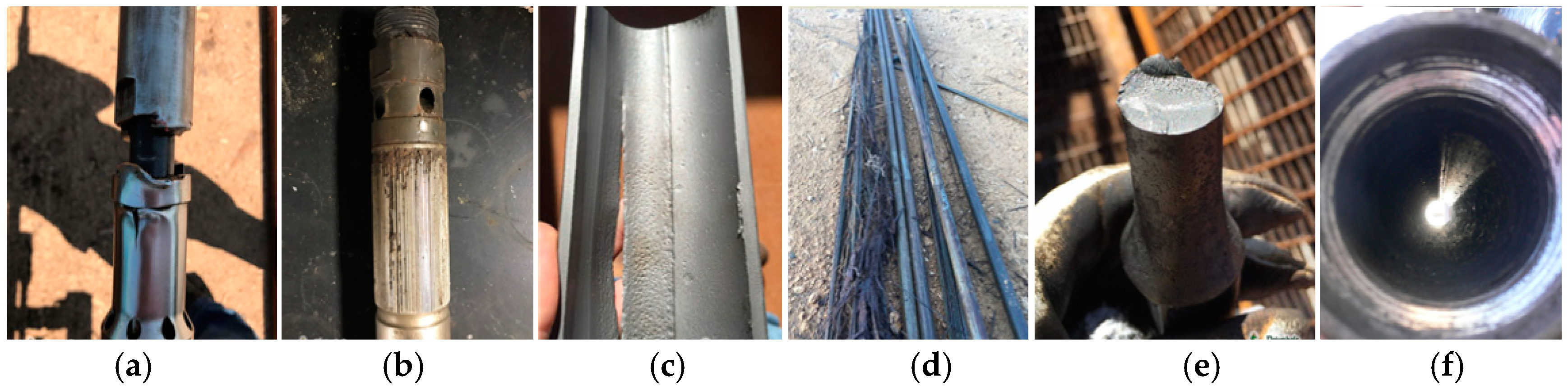
1. Introduction

Deep oil reservoirs, low permeability reservoirs, and high water cut reservoirs are deeply developed, resulting in a continuous increase in the number of deep wells, highly deviated wells, horizontal wells, and cluster wells. Concurrently, as the oil field enters the middle and later stages of production, the water cut increases year by year, and the injection medium becomes more complex. Under complex well conditions, the problems of eccentric wear of SRS and shorter pump inspection cycles are becoming more frequent. In 2018, China National Petroleum Corporation had 235,000 oil wells; the proportion of wells less than 300 days old is 25%, and the proportion of wells that exist with failure of rod, tube, and the pump is 83%. Different kinds of failure of rod, tube, and pump are shown in Figure 1. All kinds of failure of rod and tube belong to the dynamics problem of rod string in a wellbore, which is the key for optimal design and fault diagnosis of a sucker rod pumping system. As the power transmission and bearing mechanism of oil production machinery, SRS is the core equipment of the sucker rod pump. The eccentric wear and fracture of SRS impact the safety and economy of oil wells. Therefore, the study of sucker rod string mechanics has received wide attention.

The semi-empirical formula method was used to predict the load of the polished rod before 1950, but its accuracy is not very high. In 1963, Gibbs simplified the sucker rod as an elastomer and first established the longitudinal vibration equation to predict the axial load and displacement on any section of the sucker rod [1]. The mechanical model was very successful and has been widely used in oil wells. In 1990, Svinos used the concept of equivalent stiffness and equivalent density to improve the longitudinal vibration equation of rod string from single-stage sucker rod string to multi-stage sucker rod string [2]. But the error of the computational model was large. Lea aimed for further improvement in the Svinos model [3]; the Taylor series method was used to deal with the continuous conditions at the interface between adjacent rod strings, which reduced the error of calculation. In 2021, Yin used the separated variable method to solve the longitudinal vibration equation of the multistage rod string [4]. And Wang established a longitudinal vibration model for sucker rods based on a simplified thermo-solid coupled pattern and the finite element method for solving [5].

In 1983, Doty established the sucker rod and liquid longitudinal vibration coupled equation [6]. In 1995, Lelia, based on the coupled equation proposed by Doty [7], supposed that the liquid column is a single-phase incompressible liquid and developed the MacCormack explicit numerical algorithm. The calculated results were in good agreement with the measured results [8].

Aiming at the engineering problem that the casing in the oil well is not anchored, Yu established the sucker rod [9], tube, and liquid longitudinal vibration mechanics model in 1988. In 1997, Lollback found the results from the sucker rod [10], tube, and the liquid three-dimensional vibration mechanics model were close to the measured results, which proves that the model was suitable for SRS mechanics of vertical wells. In 2016, Wang successfully applied the sucker rod [11], tube, and liquid vibration equation to directional wells by using the implicit difference method at the continuous position of the sucker rod and the variable step method at couplings. In 2020, Feng successfully solved the coupled model between the high-slip motor and pumping unit according to the external characteristic function of the motor [12].

However, the above longitudinal vibration models are difficult to reveal the mechanical essence of sucker rod and tube eccentric wear, thread off of sucker rod, and other relevant problems because of having the limitations.

Aiming at the problem of eccentric wear caused by the buckling of the tubular string in the vertical well, in 2016, Huang altered the axial force of the tubular string and established the longitudinal vibration mechanical model of the tubular string [13], eventually obtaining the evolution process of the tubular string from the initial linear to 2D lateral buckling to 3D lateral buckling, then continuous contact buckling, and lastly helical buckling. In 2018, Sun established the transverse vibration model for the dynamics problem of buckling displacement excitation of sucker rod string in a vertical well [14,15]. A comprehensive calculation of the finite difference method and Newmark method was adopted, and the nonlinear dynamic simulation of the rod-tubing collision was finished. In the same year, Zhang proposed a nonlinear static slow dynamics model and an implicit finite element solution method [16].

The longitudinal vibration mechanics of SRS in a vertical well and the static buckling theory of SRS can explain part of rod and tube eccentric wear problems, but some assumptions, such as vertical wellbore trajectory and concentric rod and tube, are in disagreement with engineering practice. Ignoring the lateral force and support reaction force caused by the 3D wellbore, only referring to the static buckling force of SRS is impossible to explain the eccentric wear of the rod string above the middle location in the oil well.

In 2002, Li summarised drilling string [17], tubing and coiled tubing, sucker rod string, and casing as dynamic problems of SRS with a large slenderness ratio and studied the similarities and differences in linear and nonlinear mechanical models for the buckling of string in vertical wells and directional wells. In 2006, Lukasiewicz analysed the lateral force and helical buckling of the rod string in crude oil and confirmed the correlation between the critical helical buckling force and helical pitch [18]. In 2012, Gao established the balance equation of rod string in a horizontal well based on elasticity and beam element theory [19,20]. The equation is solved with a fourth-order Runge–Kuta method, and considering that the centraliser can effectively improve the buckling problem of SRS. In 2014, Huang established the buckling mechanical model of a rod in a horizontal well under the condition of ignoring friction [21], torque, and gravity. The 3D buckling problems were simplified into two lateral buckling problems and stressed that the influence of connectors cannot be ignored in buckling analysis.

In 2020, Moreno aimed at the mechanical analysis method about the nonlinear characteristics of Coulomb friction distribution along the wellbore trajectory in directional wells, and the method of Moreno is useful for improving the prediction ability of rod dynamic behaviour [22]. In 2021, Wang established the mathematical model of the coupled axial-transverse nonlinear vibration of SRS in directional wells and claimed that the curved wellbore trajectory is the main excitation vibration factor of SRS [23].

It is clear from the above analysis that the complete 3D curved well rod string dynamics theory can reveal and accurately predict the mechanism of rod string fatigue fracture, eccentric wear, and tripping. Whereas, when solving the complex problem in engineering, various assumptions are considered, simplifying the practical problems: the torque of SRS is ignored, which is the main cause of tripping at the rods’ connection; the spatial coordinates of 3D curved tubing are fixed; the influence of tubing non-anchoring on the change in contact position is ignored; the forced buckling influence on the 3D wellbore of SRS is not considered. Above all, the existing rod string dynamics models in 3D curved wells still have some weaknesses in predicting the mechanical behaviour of SRS with high accuracy.

In this paper, the micro-element dynamic model of the sucker rod string constrained by the actual borehole trajectory is established, the space and time are discretised using the central difference method, and the dynamometer cards are taken as the boundary condition to solve the longitudinal motion state, 3D stress state, and stress state of each point of SRS, realising an entire analysis of the overall stress and load state of SRS. By comparing the calculation results of the dynamic model with the measured data of oil wells, the accuracy and feasibility of the model are verified. The theoretical support and design reference for analysing the dynamic parameters of SRS and optimising the sucker rod pump system are provided.

2. Materials and Methods

2.1. 3D Curved Wells

The actual borehole trajectory of deep vertical wells, directional wells, and horizontal wells in the petroleum industry is an irregular 3D spatial curve with complex spatial characteristics. Wells above mentioned are collectively referred to as 3D curved wells in this paper and are shown in Figure 2. The mechanical behaviour of SRS in 3D curved wells in the borehole trajectory, where the curvature and deflection change continuously, is distinct from common wells. The super-thin rod strings bear the interaction with axial tension, torsion, and buckling, indirectly causing the deflection, wear, and breakage of SRS. During the down-hole reciprocating motion, typical geometric and nonlinear contact characteristics are displayed. 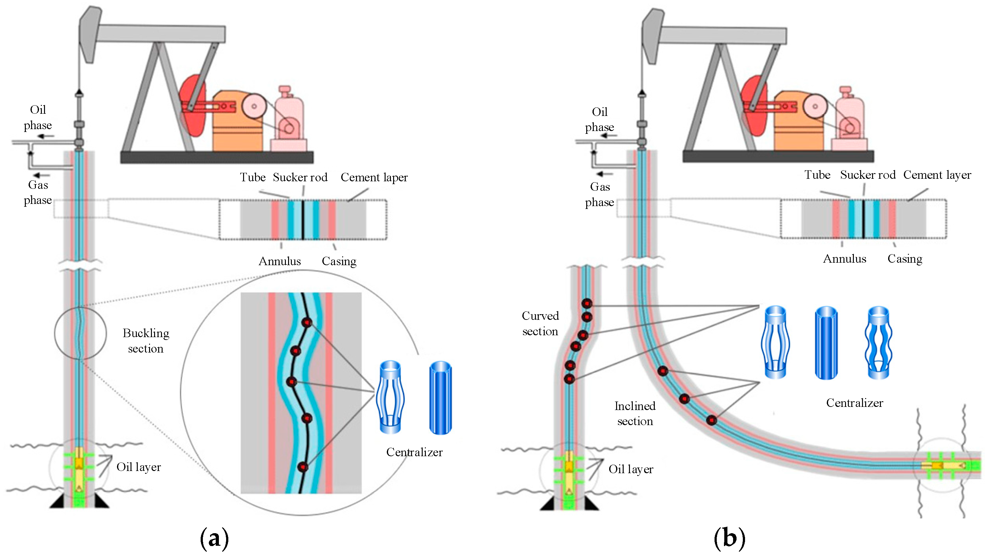Following reference [23], we will derive the mechanical model for three-dimensional curved wells.

2.2. Dynamics Model for SRS

2.2.1. Mechanical Assumptions

The dynamics model for SRS is established, which is constrained by the borehole trajectory in 3D curved wells. This model is based on some assumptions as follows:

(1)

The material of SRS is anisotropic.

(2)

SRS is treated as a complete elastomer.

(3)

SRS is circular in cross-section.

(4)

The deformation of the element is a small deformation.

(5)

The deformation processing is perpendicular to the neutral axis.

(6)

The axis of the SRS coincides with the axis of the wellbore.

(7)

The movement direction of SRS is axial and reciprocating.

(8)

The tube is anchored.

(9)

No shear stress in the cross-section of SRS.

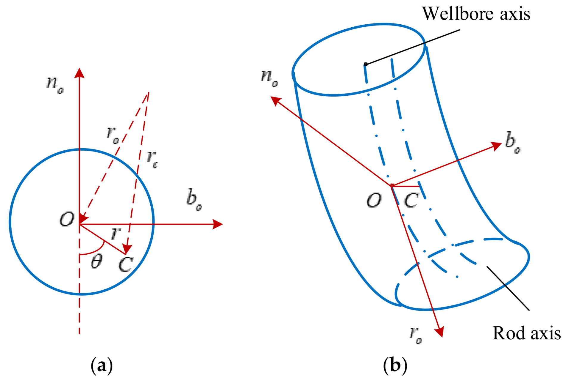
2.2.2. Geometric Description of 3D Curved Well Trajectory

Figure 3 is a geometric relationship of the 3D curved well trajectory [24]. The geometric position of any point on the wellbore axis in three-dimensional space can be described by vector diameter. Deviation angle and azimuth angle are applied to describe the tangential direction vector of the well axis trajectory. The s is the vector diameter; $r_o$ is the borehole ace length; $\alpha$ is the deviation angle; $\phi$ is the azimuth angle; and ${\tau }_o$ is the unit vector in the tangential direction.

The spatial geometric relations are formulated as follows:

$$r_o(s)=x_o(s)i+y_o(s)j+z_o(s)k,$$

(1)

$${\displaystyle \frac{d{x}_o}{ds}}=\sin \alpha \cos \phi ,$$

(2)

$${\displaystyle \frac{d{y}_o}{ds}}=\sin \alpha \sin \phi ,$$

(3)

$${\displaystyle \frac{d{z}_o}{ds}}=\cos \alpha ,$$

(4)

$${\mathsf{\tau }}_o=(\sin \alpha \cos \phi )i+(\sin \alpha \sin \phi )j+(\cos \alpha )k,$$

(5)

According to the basic principle of differential geometry, the geometric relationship between the curvature and torsion of the corresponding borehole trajectory curve, the unit vector in the tangential direction, the unit vector in the main normal direction, and the unit vector in the secondary normal direction of the borehole axis trajectory are as follows:

$$k_o=\left|{\displaystyle \frac{d{\mathsf{\tau }}_o}{ds}}\right|,T_o={\displaystyle \frac{1}{k_o^2}}\left|({\mathsf{\tau }}_o{\displaystyle \frac{d{\mathsf{\tau }}_o}{ds}}{\displaystyle \frac{d^2{\mathsf{\tau }}_o}{d{s}^2}})\right|.$$

(6)

$k_o$ is the curvature of the well trajectory curve; $T_o$ is the torsion of the well trajectory curve; $n_o$ is the unit vector in the main normal direction; and $b_o$ is the unit vector in the secondary normal direction.

Substituting Formula (5) into the above expression (6) and simplifying yields results in the following:

$$k_o^2={\left({\displaystyle \frac{d\alpha }{ds}}\right)}^2+{\sin }^2\alpha {\left({\displaystyle \frac{d\phi }{ds}}\right)}^2,$$

(7)

$$T_o={\displaystyle \frac{1}{k_o^2}}\left\{\left({\displaystyle \frac{d\alpha }{ds}}{\displaystyle \frac{d^2\phi }{d{s}^2}}-{\displaystyle \frac{d\phi }{ds}}{\displaystyle \frac{d^2\alpha }{d{s}^2}}\right)\sin \alpha +\left[2{\displaystyle \frac{d\phi }{ds}}{\left({\displaystyle \frac{d\alpha }{ds}}\right)}^2+{\sin }^2\alpha {\left({\displaystyle \frac{d\phi }{ds}}\right)}^3\right]\cos \alpha \right\},$$

(8)

$$n_o={\displaystyle \frac{1}{k_o}}[{\displaystyle \frac{d}{ds}}(\sin \alpha \cos \phi )i+{\displaystyle \frac{d}{ds}}(\sin \alpha \sin \phi )j+{\displaystyle \frac{d\cos \alpha }{ds}}k],$$

(9)

$$b_o=-{\displaystyle \frac{1}{k_o}}(\sin \phi {\displaystyle \frac{d\alpha }{ds}}+{\displaystyle \frac{\sin 2\alpha }{2}}\cdot {\displaystyle \frac{d\sin \phi }{ds}})i+{\displaystyle \frac{1}{k_o}}(\cos \phi {\displaystyle \frac{d\alpha }{ds}}+{\displaystyle \frac{\sin 2\alpha }{2}}\cdot {\displaystyle \frac{d\cos \phi }{ds}})j+({\displaystyle \frac{{\sin }^2\alpha }{k_o}}\cdot {\displaystyle \frac{d\phi }{ds}})k.$$

(10)

2.2.3. Description of the Shape of SRS Axis

The geometric relationship of SRS deformation is shown in Figure 4. The plane $O{n}_o{b}_o$ is the normal plane of the well trajectory curve at point O; point C is the intersection of the plane $O{n}_o{b}_o$ and rod axis at time t; $\theta$ is the deflection angle; $r$ is the distance from the centre of SRS in the section to the centre of the wellbore; and $r$ and $\theta$ as geometric parameters describe the three-dimensional spatial position of point C deviating from point O.

Assuming that SRS is in the regime of elastic deformation,

$${\mathsf{\tau }}_c={\displaystyle \frac{\partial r_c}{\partial s_c}}={\displaystyle \frac{ds}{d{s}_c}}[{\mathsf{\tau }}_o-{\displaystyle \frac{d(r\cos \theta )}{ds}}{n}_o+{\displaystyle \frac{d(r\sin \theta )}{ds}}{b}_o].$$

(11)

According to the basic principle of differential geometry, the geometric relationship between the curvature and torsion of the borehole trajectory curve of point C and the unit vector in the tangential direction of point C are as follows:

$$k_c=\left|{\displaystyle \frac{d{\mathsf{\tau }}_c}{ds}}\right|=\sqrt{k_o^2+r^2{\displaystyle \frac{d^2\theta }{d{s}^2}}+{({\displaystyle \frac{d\theta }{ds}})}^2},$$

(12)

$$T_c={\displaystyle \frac{1}{k_c^2}}\left|({\mathsf{\tau }}_c{\displaystyle \frac{d{\mathsf{\tau }}_c}{ds}}{\displaystyle \frac{d^2{\mathsf{\tau }}_c}{d{s}^2}})\right|={\displaystyle \frac{1}{k_c^2}}[-{\displaystyle \frac{d^2(r\cos \theta )}{d{s}^2}}{\displaystyle \frac{d^3(r\sin \theta )}{d{s}^3}}+{\displaystyle \frac{d^2(r\sin \theta )}{d{s}^2}}{\displaystyle \frac{d^3(r\cos \theta )}{d{s}^3}}].$$

(13)

2.2.4. Force Analysis of the Micro-Element of SRS

The force analysis of the micro-element of SRS is shown in Figure 5. The force problem of SRS is regarded as the longitudinal vibration problem of an elastic rod with the damper in directional wells and horizontal wells.

The loads acting on the section micro-element of SRS include internal force load moment and external force load. The external force load covers the positive pressure acting on the unit length of the micro-element, the floating weight per unit length of the micro-element, the friction between the rod and tubing, and the viscous friction of fluid acting on the unit length of the micro-element. The specific formula is as follows:

$$f_e(s)=N+q_e+f_{\lambda }+f_{\mu }.$$

(14)

$N$: the positive pressure acting on the unit length of the micro-element;

$q_e$: the floating weight per unit length of the micro-element;

$f_{\lambda }$: the friction between the rod and tubing;

$f_{\mu }$: the viscous friction of fluid acting on the unit length of the micro-element.

The deformation of SRS still belongs to the elastic deformation under the condition of down-hole limited by the tube. The shear effect is neglected during the deformation, so the constitutive equation is as follows:

$$F_e(s)=E{A}_{ro}{\displaystyle \frac{\partial u}{\partial s}},$$

(15)

$$M(s)=EI({\mathsf{\tau }}_c\times {\displaystyle \frac{\partial {\mathsf{\tau }}_c}{\partial s}}).$$

(16)

$A_{ro}$: area of section;

E: modulus of elasticity;

I: section moment of inertia.

2.2.5. Dynamic Differential Equation of SRS

The microelement balance equation of SRS is

$$F_e(s+ds)-F_e(s)+f_e(s)ds=\rho A{\displaystyle \frac{{\partial }^{2}u(s,t)}{\partial t^2}}{\mathsf{\tau }}_{c}ds.$$

(17)

Dividing $ds$ on both sides of the equation, then Equation (17) is transformed into Equation (18).

$${\displaystyle \frac{\partial F_e(s)}{\partial s}}+f_e(s)=\rho A{\displaystyle \frac{{\partial }^{2}u(s,t)}{\partial t^2}}{\tau }_c.$$

(18)

According to the theorem of momentum moment, the momentum moment of micro element at time t is

$${\displaystyle \frac{\partial M(s)}{\partial s}}+{\mathsf{\tau }}_c\times F_e(s)=0.$$

(19)

The dynamics differential equation of SRS is obtained by combining the above formula as follows:

$$\begin{array}{l}\rho A{\displaystyle \frac{{\partial }^{2}u}{\partial t^2}}+[f\sqrt{N_n^2+N_b^2}/\left|{\displaystyle \frac{\partial u}{\partial t}}\right|+\pi {\mu }_o{\displaystyle \frac{m^2-1}{(m^2+1)\ln m-(m^2-1)}}+{\displaystyle \frac{8\pi {\mu }_i}{A_{\mathit{ri}}}}]{\displaystyle \frac{\partial u}{\partial t}}\\ =EA{\displaystyle \frac{{\partial }^{2}u}{\partial l^2}}+EI{\displaystyle \frac{\partial k_c}{\partial l}}{k}_c+q_{e\tau }+{\displaystyle \frac{8\pi {\mu }_i}{A_{ri}}}{V}_i-\pi {\mu }_o{\displaystyle \frac{m^2-1}{(m^2+1)\ln m-(m^2-1)}}\left|{\displaystyle \frac{\partial u}{\partial t}}\right|\end{array},$$

(20)

$$m={\left({\displaystyle \frac{A_t}{A_{ro}}}\right)}^{0.5},$$

(21)

$$EI{\displaystyle \frac{{\partial }^2{k}_c}{\partial s^2}}-EI{k}_c{T}_c^2-EA{\displaystyle \frac{\partial u}{\partial s}}{k}_c-q_{en}=N_n,$$

(22)

$$EI{\displaystyle \frac{\partial T_c}{\partial s}}{k}_c+2EI{\displaystyle \frac{\partial k_c}{\partial s}}{T}_c-q_{eb}=N_b.$$

(23)

$A_t$: the cross-sectional area of the oil tube;

$A$: the cross-sectional area of the sucker rod;

m: dimensionless number;

$\rho$: the density of the sucker rod;

$N_n$: the support reaction force in the main normal direction of the micro-element;

$N_b$: the support reaction force in the direction of the sub-normal of the micro-element;

$f$: friction coefficient;

${\mu }_o$: the outside fluid’s dynamic viscosity of the sucker rod;

${\mu }_i$: the inside fluid’s dynamic viscosity of the sucker rod;

$V_i$: the fluid’s average velocity of the sucker rod.

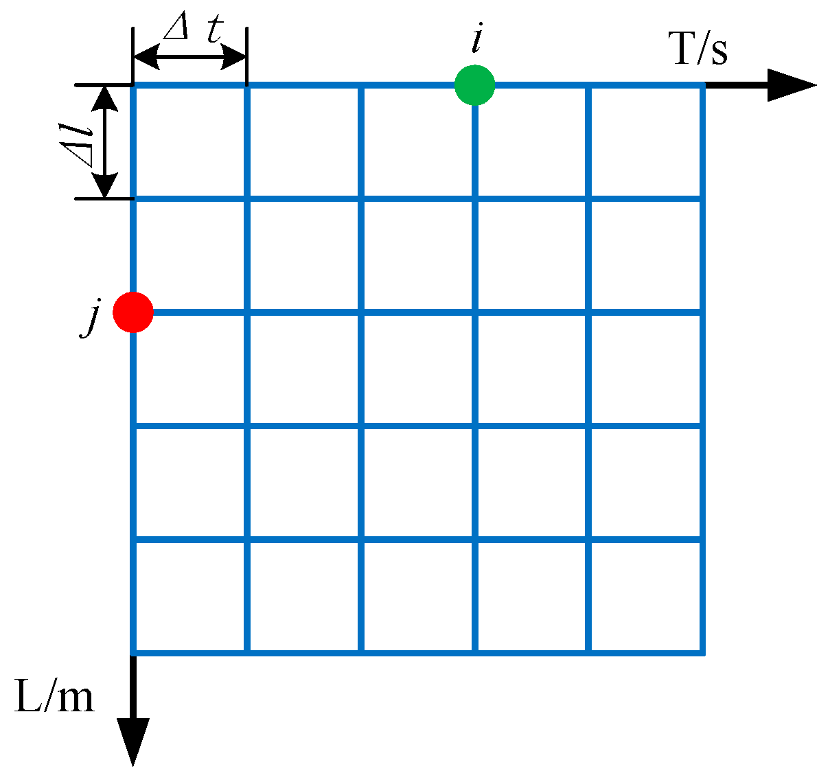
2.2.6. Solution of Dynamic Model of Sucker Rod String

In this paper, the central difference method is used to discretise the SRS dynamics model. The numerical difference grid is shown in Figure 6. The vertical coordinate represents the well depth, and each node is represented by i totals of nodes, which is n + 1, and the step length is $\Delta l$. The horizontal coordinate is the motion period T, the node is represented by j, and the step length is $\Delta t$. To ensure the success of convergence, this formula must be satisfied, that is, ${\displaystyle \frac{\Delta l}{\zeta \Delta t}}<1$ and $\zeta =\sqrt{E/\rho }$. In Figure 6, the green dot (i) represents a calculation point in the time direction, while the red dot (j) represents a calculation point in the spatial direction. These two dots are used in the numerical difference grid to indicate different calculation positions.

The discrete forms of SRS dynamics model are as follows:

$$\begin{array}{l}({\displaystyle \frac{{\rho }_i{A}_i}{\Delta t^2}}-{\displaystyle \frac{a_{i,j}}{\Delta t}})u_{i,j-1}-({\displaystyle \frac{2{\rho }_i{A}_i}{\Delta t^2}}+{\displaystyle \frac{E_i{A}_i}{\Delta l^2}}-{\displaystyle \frac{a_{i,j}}{\Delta t}})u_{i,j}+{\displaystyle \frac{{\rho }_i{A}_i}{\Delta t^2}}{u}_{i,j+1}\\ =E_i{A}_i{\displaystyle \frac{u_{i-2,j}-2u_{i-1,j}}{\Delta l^2}}+E_i{I}_i({\displaystyle \frac{k_{ci}-k_{ci-1}}{l_i-l_{i-1}}})k_{ci}+{\varsigma }_{ij}\end{array},$$

(24)

$$E_i{I}_i{\displaystyle \frac{k_{ci}-k_{ci-1}}{l_i-l_{i-1}}}-E_i{I}_i{k}_{ci}{T}_{ci}^2-E_{i-1}{A}_{i-1}{\displaystyle \frac{u_{i-1,j}-u_{i-2,j}}{\Delta l}}{k}_{ci}-q_{eni}=N_{ni},$$

(25)

$$E_i{I}_i{\displaystyle \frac{T_{ci}-T_{ci-1}}{l_i-l_{i-1}}}{k}_{ci}+2E_i{I}_i{\displaystyle \frac{k_{ci}-k_{ci-1}}{l_i-l_{i-1}}}{T}_{ci}-q_{ebi}=N_{bi},$$

(26)

$$a_{i,j}=f\sqrt{N_{ni}^2+N_{bi}^2}/\left|{\displaystyle \frac{u_{i-1,j}-u_{i-1,j-1}}{\Delta t}}\right|+\pi {\mu }_o{\displaystyle \frac{m_i^2-1}{(m_i^2+1)\ln m_i-(m_i^2-1)}}+{\displaystyle \frac{8\pi {\mu }_i}{A_{ri}}},$$

(27)

$${\varsigma }_i=q_{e\tau ,i}+{\displaystyle \frac{8\pi {\mu }_i}{A_{ri}}}{V}_i-\pi {\mu }_o{\displaystyle \frac{m_i^2-1}{(m_i^2+1)\ln m_i-(m_i^2-1)}}\left|{\displaystyle \frac{u_{i-1,j}-u_{i-1,j-1}}{\Delta t}}\right|.$$

(28)

2.2.7. Continuity and Initial Conditions of Discrete Form of Dynamics Model

(1)

Continuity conditions

If there is a sudden change in the cross-section of the oil extraction rod at depth $l_i$, the section above point $l_i$ is the $k$-th level rod with a cross-sectional area of $A_{i,k}$ and an elastic modulus of $E_{i,k}$, and its position at time $j$ is $u_{i,j,k}$; the section below point $l_i$ is the $k+1$-th level rod with a cross-sectional area of $A_{i,k+1}$ and an elastic modulus of $E_{i,k+1}$, and its position is $u_{i,j,k+1}$. The following displacement and axial force continuity conditions apply:

$$u_{i,j,k}=u_{i,j,k+1},$$

(29)

$$E_{i,k}{A}_{i,k}{\displaystyle \frac{u_{i,j,k}-u_{i-1,j,k}}{\Delta l}}=E_{i+1,j,k+1}{A}_{i+1,k+1}{\displaystyle \frac{u_{i+1,j,k+1}-u_{i,j,k+1}}{\Delta t}}-{\rho }_{o}g{l}_i(A_{i,k+1}-A_{i,k}).$$

(30)

(2)

Initial conditions

$$u_{i,j}=u_{i,j+1}=u_{i,j-1}.$$

(31)

$${\displaystyle \frac{u_{i,j}-u_{i,j-1}}{\Delta t}}={\displaystyle \frac{u_{i,j+1}-u_{i,j}}{\Delta t}}={\displaystyle \frac{u_{i,j-1}-u_{i,j-2}}{\Delta t}}.$$

(32)

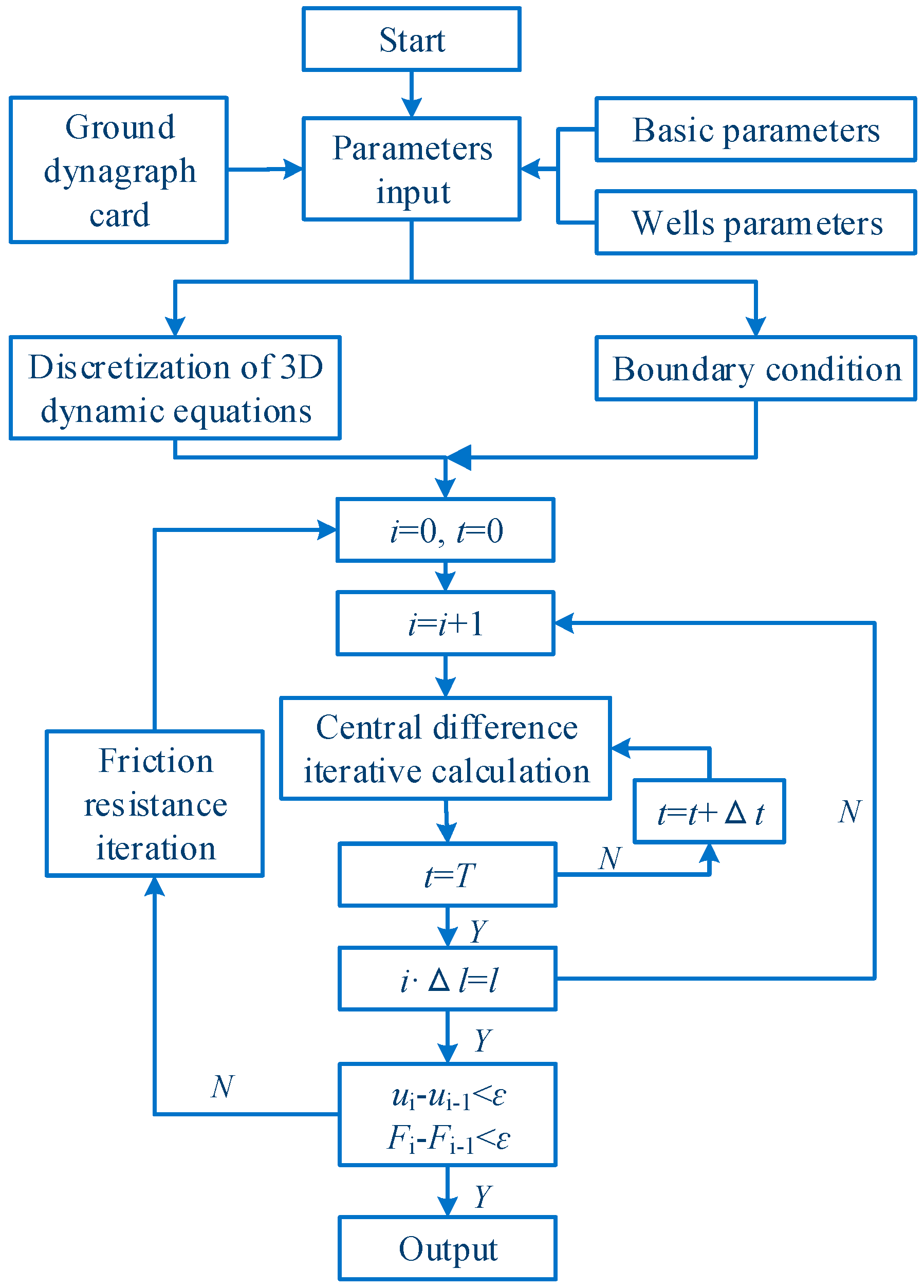
2.2.8. Calculation Process

The motion processing of SRS is analysed, and the dynamometer cards are taken as the boundary condition; the input node’s load and displacement of the initial element are solved iteratively according to the discrete forms of the SRS dynamics model. Then, the displacement, transverse force, bending moment, and axial force of each element node are solved one by one. Finally, the stress and the bearing load of each node are obtained. $\epsilon$ represents a very small positive number used to control errors or determine the precision of numerical calculations. The iterative calculation process is shown in Figure 7.

3. Optimisation Design Method for the Arrangement of Centralisers

The arrangement of centralisers is a critical aspect of sucker rod string design, with the primary objectives of reducing rod-tubing wear, improving system efficiency, and extending the service life of the equipment.

Common design methods for sucker rod centralisers in oilfields are as follows: The sucker rod string is simplified as a slender, simply supported beam, with the suspension point and the upper end of the pump serving as two simple supports while ignoring the effects of rod string torsion and the three-dimensional wellbore. Axial loads and lateral forces on the sucker rod string are analysed. Based on the theory of elasticity, a buckling equation for the rod string is established to analyse its buckling behaviour under axial loads and lateral forces, determining the deformation curve of the rod string. Using the solution of the buckling equation, the contact points between the rod string and the tubing are calculated. These contact points typically occur in areas with significant lateral forces (such as curved or horizontal sections of the wellbore). Centralisers are then positioned at the contact points between the rod string and the tubing.

The traditional design method for centralisers is simple and practical, making it suitable for vertical wells and some directional wells. However, this traditional method does not account for three-dimensional wellbore trajectories, rod string torque effects, or dynamic behaviour, resulting in limited applicability under complex well conditions.

This article addresses the limitations of traditional centraliser design methods under complex well conditions and proposes a centraliser design theory and method based on a three-dimensional mechanical coupling mathematical model. This method comprehensively considers the dynamic behaviour of the sucker rod string, wellbore trajectory, and complex loading conditions, optimising the placement and spacing of centralisers to enhance system efficiency and reduce eccentric wear.

The optimised design process for the centraliser proposed in this article is as follows:

(1)

Collecting well conditions and design parameters: Inputting data such as wellbore trajectory, rod string parameters, and fluid column characteristics to provide a foundation for model calculations.

(2)

Establishing a three-dimensional mechanical coupling mathematical model: Taking into account the axial load, lateral forces, torque effects on the sucker rod string, and the three-dimensional curvature of the wellbore trajectory.

(3)

Calculating the stress state of the rod string: Using the model to calculate the axial load, lateral force distribution, and dynamic stress conditions of the rod string.

(4)

Analysing the buckling behaviour of the rod string: Studying the buckling forms of the rod string under different load conditions (e.g., two-dimensional buckling, three-dimensional helical buckling).

(5)

Determining the contact points between the rod string and the tubing: Calculating the positions of contact points between the rod string and the tubing based on the stress and buckling analysis results.

(6)

Optimising the placement of centralisers: Prioritising placing centralisers in areas with contact points and high lateral forces.

(7)

Dynamically adjusting the spacing of centraliser placement: Adjusting the spacing of centralisers dynamically based on the wellbore curvature and the stress distribution of the rod string, avoiding the limitations of fixed-spacing designs.

(8)

Validating the design: Checking whether the centraliser placement effectively reduces wear and buckling, ensuring the design meets the requirements of actual well conditions.

(9)

Adjusting model parameters and re-optimising: If the design does not meet the requirements, model parameters must be adjusted (e.g., rod string diameter, number of centralisers), and the placement re-optimised.

(10)

Finalising the design: Outputting the placement positions and spacing of the centralisers, along with the stress and wear analysis results of the rod string.

4. Comparative Analysis of Application Cases

To validate the effectiveness, applicability, and practical performance of the centraliser design theory and methods proposed in this paper, two oil wells (A1#, A2#) were selected for optimised centraliser design. At the same time, by comparing with the traditional centraliser design methods used in the oilfield [25], it is hoped to demonstrate the advantages of the methods presented in this paper.

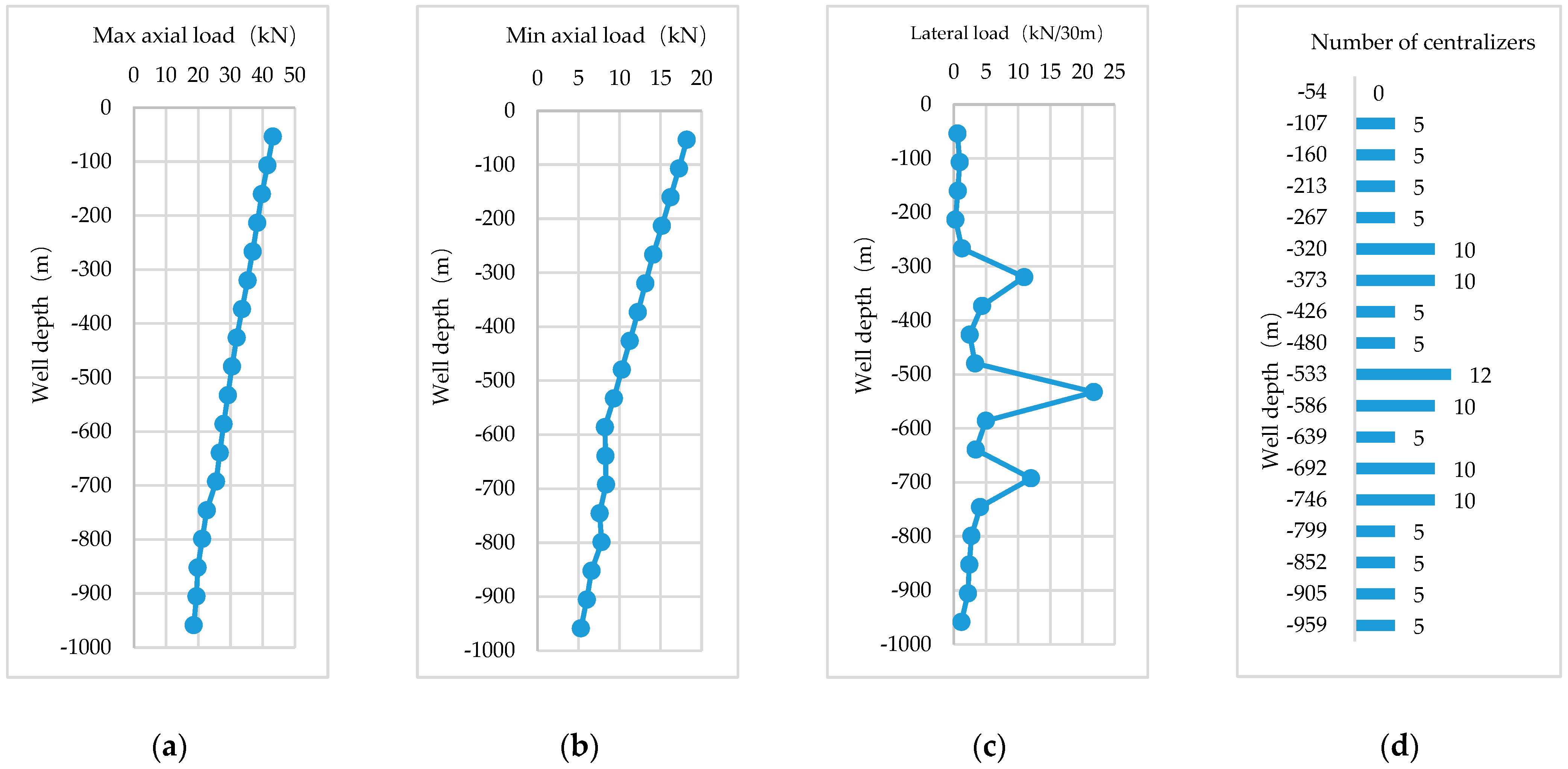
4.1. Experiment Case 1. A1# Oil Well Engineering Design

Application example 1 is A1# oil well of an oil production plant in Daqing Oilfield as shown in

Table 1. Basic design parameters of oil wells (oil well A1#).

Specific Elements	Unit	Data
Medium-deep oil layer	m	990.6
Relative density of crude oil	%	0.85
Production gas oil ratio	m3/m3	10.00
Casing inner diameter	mm	124.00
Formation pressure	MPa	10.53
Relative density of formation water	%	1.00
Water cut	%	0.99
Inner diameter of oil pipe	mm	76.00
Reservoir temperature	°C	54.62
Relative density of natural gas	%	0.70

. The A1# oil well is located in a medium-deep oil reservoir, with a well depth of 990.6 metres. It exhibits relatively high formation pressure (10.53 MPa) and moderate formation temperature (54.62 °C). The produced fluid is predominantly characterised by a high water cut (99%), and the crude oil has a relative density of 0.85, classifying it as light crude oil. The associated gas production is relatively low, with a gas-oil ratio of 10.00 m³/m³. The wellbore structure is designed appropriately, with a casing inner diameter of 124.00 mm and a tubing inner diameter of 76.00 mm, making it suitable for production during the high water cut phase.

The production performance of oil well A1# after arranging centralisers according to the traditional design method is as follows (as shown in

Table 2. Design results of traditional methods (oil well A1#).

Specific Elements	Unit	Data
Stroke	m	4.20
Pump diameter	mm	38.00
Pump efficiency	%	47.78
Rod diameter	mm	19
Frequency of stroke	Hz	6.00
Pump depth	m	900.05
System efficiency	%	15
Liquid production	m3	19.65
Dynamic liquid level depth	m	650
Submergence	m	250.05
Maximum load	KN	28.07

): This well utilises a pumping system with a stroke length of 4.20 m, a pump diameter of 38 mm, and a stroke frequency of 6.00 Hz, with the pump set at a depth of 900.05 m. Under these design operating conditions, the pump efficiency is 47.78%, and the system efficiency is relatively low at only 15%, with a daily liquid production of 19.65 m³. The dynamic liquid level is at a depth of 650 m, with a liquid submergence depth of 250.05 m, and the maximum load is 28.07 kN. Overall, the traditional centraliser arrangement design has failed to effectively improve system efficiency, with both pump efficiency and liquid production remaining low, indicating room for further optimisation.

The production status of oil well A1# after designing the centraliser arrangement according to the method described in this paper is as follows (as shown in

Table 3. Design and results of the methodology in this paper (oil well A1#).

Specific Elements	Unit	Data
Stroke	m	4.20
Pump diameter	mm	38.00
Pump efficiency	%	47.78
Rod diameter	mm	19
Frequency of stroke	Hz	6.00
Pump depth	m	900.05
System efficiency	%	20
Liquid production	m3	19.65
Dynamic liquid level depth	m	600
Submergence	m	300.05
Maximum load	KN	24.52

): The well continues to use a pumping system with a stroke length of 4.20 m, a pump diameter of 38 mm, and a stroke frequency of 6.00 Hz, with a pump setting depth of 900.05 m. Under this design, the pump efficiency remains at 47.78%, but the system efficiency has increased to 20%, and the daily liquid production is maintained at 19.65 m³. The dynamic liquid level has risen to 600 m, with the submergence depth increasing to 300.05 m, and the maximum load reduced to 24.52 kN. Overall, the centraliser arrangement designed using the method described in this paper has effectively improved system efficiency, reduced rod string load, and optimised production performance, demonstrating superior design results.

The production status changes in oil well A1# under the traditional design method and the design method proposed in this paper are as follows: system efficiency increased by 5 percentage points, indicating a significant improvement; the dynamic liquid level depth rose from 650 m to 600 m, with a 20% increase in submergence; the maximum load was reduced by 12.65%, demonstrating an optimisation of the rod string’s stress conditions. Pump efficiency and daily liquid production remained unchanged. The design method proposed in this paper significantly enhanced system efficiency, improved liquid level conditions, and reduced rod string load through the optimisation of centraliser arrangement, effectively improving overall production performance and operational stability.

Figure 8a shows the distribution of the maximum load of SRS in the A1# well along with the well depth, and Figure 8b shows the distribution of the minimum load of SRS in the A1# well rod along with the well depth. It can be seen from Figure 8a,b that the distribution law of maximum load and minimum load with well depth is the same, and the larger the well depth is, the smaller the load is. The reason is that the deeper the well is, the less the influence of the gravity of SRS on the axial force is. In addition, the liquid column pressure is also gradually decreasing, so the axial force on the SRS is also smaller.

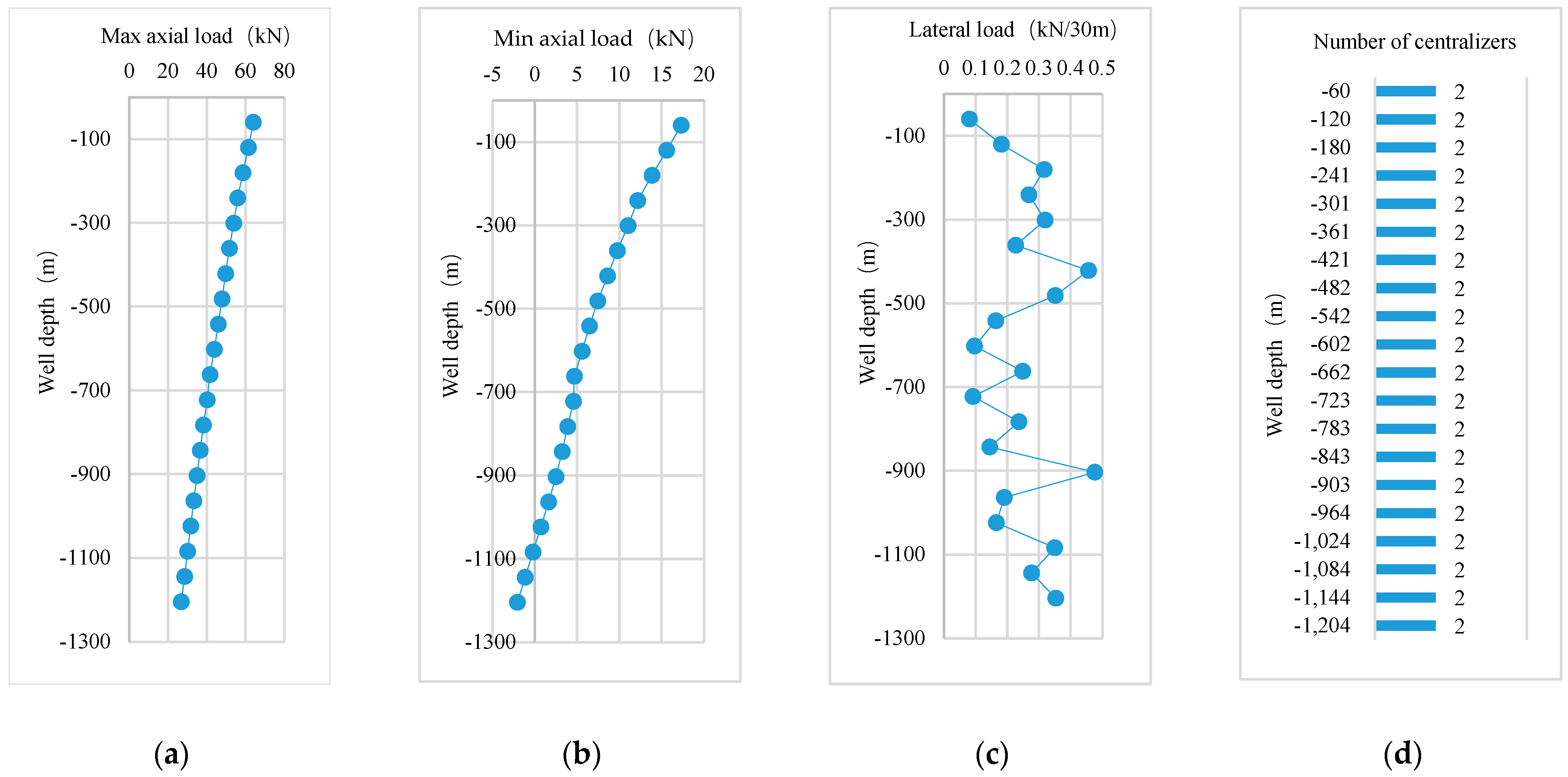
4.2. Experiment Case 2. A2# Oil Well Engineering Design

Application example 2 is A2# well of an oil production plant in Daqing Oilfield. The parameters are shown in Table 1, Table 2 and Table 3. The matching pump depth is 992.33 m, and the pump type is φ 57 mm; the inner diameter of the oil pipe is 0.076 m. The length of the sucker rod is 971.41 m, the stroke of the sucker pumping unit is 4.2 m, and the frequency of strokes is 4 times/min (as shown in

Table 4. Basic design parameters of oil wells (oil well A2#).

Specific Elements	Unit	Data
Medium-deep oil layer	m	1057
Relative density of crude oil	%	85
Production gas oil ratio	m3/m3	10.0
Casing inner diameter	mm	124.0
Formation pressure	MPa	10
Relative density of formation water	%	100
Water cut	%	89
Inner diameter of oil pipe	mm	76.0
Reservoir temperature	°C	53.35
Relative density of natural gas	%	70

).

The production performance of oil well A2# under the traditional centraliser design method is as follows (as shown in

Table 5. Design results of traditional methods (oil well A2#).

Specific Elements	Unit	Data
Stroke	m	4.20
Pump diameter	mm	70.00
Pump efficiency	%	39.8
Rod diameter	mm	25
Frequency of stroke	Hz	4.00
Pump depth	m	992.3
System efficiency	%	33.4
Liquid production	m3	36.39
Dynamic liquid level depth	m	961.88
Submergence	m	30.45
Maximum load	KN	56.45

): This well employs a pumping system with a stroke length of 4.20 m, a pump diameter of 70 mm, and a stroke frequency of 4.00 Hz, with a pump setting depth of 992.3 m. Under these design conditions, the pump efficiency is 39.8%, the system efficiency is 33.4%, and the daily liquid production is 36.39 m³. The dynamic liquid level depth is 961.88 m, with a submergence depth of only 30.45 m. Overall, the production performance under the traditional centraliser design method demonstrates relatively low pump efficiency and system efficiency, along with insufficient submergence depth, which may affect the stable operation of the pump and production efficiency. There is potential for further optimisation.

The production status of oil well A2# under the centraliser design measures proposed in this paper is as follows (as shown in

Table 6. Design and results of the methodology in this paper (oil well A2#).

Specific Elements	Unit	Data
Stroke	m	4.20
Pump diameter	mm	57.00
Pump efficiency	%	58.9
Rod diameter	mm	22
Frequency of stroke	Hz	4.00
Pump depth	m	992.3
System efficiency	%	35
Liquid production	m3	36.39
Dynamic liquid level depth	m	700
Submergence	m	292.33
Maximum load	KN	51.23

): This well utilises an oil extraction system with a stroke length of 4.20 m, a pump diameter of 57 mm, and a stroke frequency of 4.00 Hz, with the pump set at a depth of 992.3 m. Under these design conditions, the pump efficiency has significantly improved to 58.9%, and system efficiency has increased to 35%, while the daily liquid production remains at 36.39 m³. The dynamic liquid level has risen to 700 m, and the submergence depth has increased to 292.33 m. The maximum load is 51.23 kN, and the minimum load is 14.25 kN. Overall, the design measures presented in this paper have optimised the arrangement of the centralisers, significantly enhancing pump efficiency and system efficiency, improving the submergence depth, reducing the operational risks of the pump, and increasing production stability and efficiency.

Comparing the production performance of oil well A2# under the traditional design method and the design method proposed in this study, the changes in various parameters are as follows: Pump efficiency increased by 19.1 percentage points; system efficiency improved by 1.6 percentage points, with a relatively small increase; the dynamic liquid level depth significantly rose from 961.88 m to 700 m, with the submergence depth increasing nearly 9.6 times; the maximum load decreased by 9.24%, indicating a more reasonable force distribution in the rod string. The design method proposed in this study has significantly optimised pump efficiency, liquid level conditions, and load distribution, resulting in a marked improvement in overall production efficiency and operational stability.

After three-dimensional mechanical design and calculation of SRS, the results are shown in Figure 9. It can be obtained from Figure 9a,b that maximum and minimum axial loads decrease with the well depth, which is mainly affected by the weight of SRS and the weight of the liquid column, but the minimum value is negative after 1084 m. It should be observed whether the pump jacking phenomenon occurs. From Figure 9c, there are several maxima of the lateral force of SRS along the well depth after 420 m, 900 m, and 1000 m. However, compared with case 1, the difference in the lateral force is small, and the effect of the centraliser is obvious. In Figure 9d, within the whole well depth, due to the small maximum amplitude of lateral force and the small difference in lateral force at each position, centralisers are set at 2/60 m, which are evenly distributed.

5. Conclusions

(1)

To solve the problems of SRS being prone to breakage and deflection in 3D curved wells, the mechanically coupled mathematical model of SRS in 3D curved wells is established. The central difference method is applied to solve the problem. In the solution procedure, the micro SRS element is taken as the force unit, while the influence of the elastic force, inertia force, and friction are included. The well trajectory, rod string structure, and tubing are treated as the external conditions.

(2)

The motion state and 3D stress–strain distribution of each point on SRS, as well as the location of the centraliser arrangement, are obtained by the proposed new dynamics model.

(3)

In the DaQing oilfield, the mechanically coupled mathematical model was applied to design the centraliser arrangement for two oil wells, achieving significant improvements in production performance. For the A1# oil well, the rod diameter was reduced from 22 mm to 19 mm, the maximum load decreased by 11.4% (from 27.67 kN to 24.52 kN), and the minimum load decreased by 9.3% (from 15.15 kN to 13.74 kN). The system efficiency increased by 25% (from 16% to 20%), and the pumping efficiency remained stable. For the A2# oil well, the pumping efficiency increased by 47.9% (from 39.8% to 58.9%), the system efficiency improved by 4.8% (from 33.4% to 35%), and the submergence depth increased by 860% (from 30.45 m to 292.33 m). This method, proposed in the study, overcomes the limitations of traditional approaches under complex well conditions through precise mathematical modelling and optimised design, significantly enhancing system efficiency, oil extraction efficiency, and production stability.

(4)

The practical oil well application shows that the arrangement of centralisers in the well section where the rod and tube deviation wear can improve the stability of the sucker rod pumping system, reduce the load of the suspension point, and improve the system efficiency.

References

- Gibbs, S.G. Predicting the behavior of sucker rod pumping systems. J. Pet. Technol. 1963, 15, 769–778. [Google Scholar] [CrossRef]
- Svinos, J.G. Rodstar—An expert rod pumping system predictive simulator. In Proceedings of the Annual Technical Meeting, Calgary, AB, Canada, 10–13 June 1990; pp. 1–18. [Google Scholar] [CrossRef]
- Lea, J.F. Boundary Conditions Used with Dynamic Models of Beam Pump Performance; Chicago, United States, Amoco Production Company, Southwestern Petroleum Short Course: Chicago, IL, USA, 1988; pp. 251–263. [Google Scholar]
- Yin, J.J.; Sun, D.; Yang, Y.S. Predicting multi-tapered sucker-rod pumping systems with the analytical solution. J. Pet. Sci. Eng. 2021, 197, 108115. [Google Scholar] [CrossRef]
- Wang, X.B.; Lv, L.Q.; Li, S.; Pu, H.; Liu, Y.; Bian, B.; Li, D. Longitudinal vibration analysis of sucker rod based on a simplified thermo-solid model. J. Pet. Sci. Eng. 2021, 196, 107951. [Google Scholar] [CrossRef]
- Doty, D.R.; Schmidt, Z. An Improved Model for Sucker Rod Pumping. Soc. Pet. Eng. J. 1983, 23, 33–41. [Google Scholar] [CrossRef]
- Lelia, S.D.L.; Evans, R.D. A coupled rod and fluid dynamic model for predicting the behavior of sucker-rod pumping systems. SPE Prod. Facil. 1995, 10, 26–33. [Google Scholar] [CrossRef]
- Lelia, S.D.L.; Evans, R.D. A coupled rod and fluid dynamic model for prediction the behavior of sucker-rod pumping systems-Part 2: Parametric study and demonstration of model capabilities. SPE Prod. Facil. 1995, 10, 34–40. [Google Scholar] [CrossRef]
- Yu, G.A.; Wu, Y.J.; Wang, G.Y. Three dimensional vibration in a sucker rod beam pumping system. Acta Pet. Sin. 1989, 10, 76–82. [Google Scholar]
- Lollback, P.A.; Wang, G.Y.; Rahman, S.S. An alternative approach to the analysis of sucker-rod dynamics in vertical and deviated wells. J. Pet. Sci. Eng. 1997, 17, 313–320. [Google Scholar] [CrossRef]
- Wang, D.; Liu, H. Dynamic modeling and analysis of sucker rod pumping system in a directional well. In Mechanism and Machine Science; Springer: Singapore, 2016; pp. 1115–1127. [Google Scholar] [CrossRef]
- Feng, Z.M.; Ma, Q.Y.; Liu, X.L.; Cui, W.; Tan, C.D.; Liu, Y. Dynamic coupling modelling and application case analysis of high-slip motors and pumping units. PLoS ONE 2020, 15, e0227827. [Google Scholar] [CrossRef]
- Huang, W.J.; Gao, D.L.; Liu, Y.H. A study of tubular string buckling in vertical wells. Int. J. Mech. Sci. 2016, 118, 231–253. [Google Scholar] [CrossRef]
- Sun, X.R.; Jiang, S.B.; Huang, Y.Q.; Yao, H.T.; Li, S.F.; Dong, S.M. Simulation research of transverse vibration of sucker rod string under buckling deformation excitation in vertical wells. J. Vib. Eng. 2018, 31, 854–861. [Google Scholar] [CrossRef]
- Sun, X.R.; Dong, S.M.; Wang, H.B.; Li, W.C.; Sun, L. Comparison of multistage simulation models of entire sucker rod with spatial buckling in tubing. J. Jilin Univ. (Eng. Technol. Ed.) 2018, 48, 153–161. [Google Scholar] [CrossRef]
- Zhang, Q.; Jiang, B.; Huang, W.J.; Cui, W.; Liu, J.B. Effect of wellhead tension on buckling load of tubular strings in vertical wells. J. Pet. Sci. Eng. 2018, 164, 351–361. [Google Scholar] [CrossRef]
- Li, Z.F.; Li, J.Y. Fundamental equations for dynamic analysis of rod and pipe string in oil-gas wells and application in static buckling analysis. J. Can. Pet. Technol. 2002, 41, 44–53. [Google Scholar] [CrossRef]
- Lukasiewicz, S.A.; Knight, C. On lateral and helical buckling of a rod in a tubing. J. Can. Pet. Technol. 2006, 44, 17–21. [Google Scholar] [CrossRef]
- Gao, G.H.; Di, Q.F.; Miska, S.; Wang, W.H. Stability analysis of pipe with connectors in horizontal wells. SPE J. 2012, 17, 931–941. [Google Scholar] [CrossRef]
- Gao, D.L.; Huang, W.J. A review of down-hole tubular string buckling in well engineering. Pet. Sci. 2015, 12, 443–457. [Google Scholar] [CrossRef]
- Huang, W.J.; Gao, D.L. Helical buckling of a thin rod with connectors constrained in a cylinder. Int. J. Mech. Sci. 2014, 84, 89–198. [Google Scholar] [CrossRef]
- Moreno, G.A.; Garriz, A.E. Sucker rod string dynamics in deviated wells. J. Pet. Sci. Eng. 2020, 184, 106534. [Google Scholar] [CrossRef]
- Wang, H.B.; Dong, S.M. Research on the coupled axial-transverse nonlinear vibration of sucker rod string in deviated wells. J. Vib. Eng. Technol. 2021, 9, 115–129. [Google Scholar] [CrossRef]
- Wang, W.C. Research and Application of Dynamic Characteristics Analysis Method for Sucker Rod String in Three-Dimensional Curved Wells. Ph.D. Thesis, Shanghai University, Shanghai, China, 2011. [Google Scholar]
- Wang, W.C.; Bai, N.; Di, Q.F.; Wang, M.J.; Sheng, L.M.; Yang, X.K. A new method in designing position of centralizers of sucker rod strings in 3D directional wellbores. Drill. Prod. Technol. 2015, 38, 49–52+9. [Google Scholar] [CrossRef]