Abstract
In decentralized scenarios without fully trustable parties (e.g., in mobile edge computing or IoT environments), the shuffle model has recently emerged as a promising paradigm for differentially private federated learning. Despite many efforts of privacy accounting for federated learning with many sequential rounds in the shuffle model, they suffer from generality and tightness. For example, existing accounting methods are targeted to single-message shuffle protocols (which have intrinsic utility barriers compared to multi-message ones), and are untight for the commonly used vector randomized response randomizer. As countermeasures, we first present a tight total variation characterization of vector randomized response randomizers in the shuffle model, which demonstrates over 20% budget conservation. We then unify the representation of single-message and multi-message shuffle protocols and derive their privacy loss distribution (PLD). The PLDs are finally composed by Fourier analysis to obtain the overall privacy loss of many sequential rounds in the shuffle model. Through simulations in federated decision tree building and federated deep learning, we show that our approach saves up to 80% budget when compared to existing methods.
1. Introduction
Federated analytics and federated learning leverage data from multiple sources (e.g., individuals and organizations) to empower data mining and learning applications. They do not access the raw data to alleviate privacy concerns, allowing participants to contribute only summary statistics or intermediate information (e.g., gradient vectors). However, recent studies have demonstrated that summary statistics might still reveal sensitive attributes [1], and that the intermediate gradient vectors can be used to reconstruct raw data with high precision [2]. As a countermeasure, it is necessary to incorporate federated analytics and learning with theoretically rigorous notions of privacy protection (e.g., the de facto standard of differential privacy [3]).
In federated settings, the shuffle model has emerged as one of the most appealing paradigms of differential privacy, showing excellent privacy–utility–complexity trade-offs and attracting much attention from both academia and industry [4,5]. In the shuffle model, messages from users are first randomized locally, then anonymized and permuted by a shuffler, which can be implemented by anonymous channels, edge servers, or a set of non-colluding assisting parties. Since the server or statistician only observes shuffled messages, participants benefit from privacy amplification via shuffling [6]. That is, although the messages from each participant have low privacy protection (with little randomization noise), anonymously hiding among shuffled messages ensures stronger privacy protection. For example, shuffled -LDP messages from n users satisfy -DP [7].
Much effort has been devoted to one-round privacy amplification analyses in the shuffle model (e.g., [6,7,8,9]), which is a key ingredient for achieving excellent privacy–utility–complexity trade-offs in one-time data queries (e.g., distribution estimation and numerical value summation). Meanwhile, in federated analytics and learning tasks, there are normally multiple queries, and many depend on previous querying results, such as in frequent itemset mining, decision trees, and federated deep learning. It is urgent to derive tight sequential composition in the shuffle model (to obtain desirable privacy–utility trade-offs), but this can be challenging as the noise distributions involved can be sophisticated. The work of [10] resorts to Rényi differential privacy to approximate the Rényi divergence bound in the shuffle model with LDP messages. However, Rényi DP itself may not be tight under composition [11], and the Rényi divergence bound is overestimated for the noise distributions in shuffle protocols. A more recent work directly numerically analyzes the approximate privacy loss distribution of the shuffled LDP messages and derives tighter composition bounds via Fourier analysis, based on the clone reduction [8] of LDP messages. Nevertheless, their analysis is restricted to the single-message shuffle protocols (i.e., shuffled LDP messages), which suffer utility limitations compared to the more general multi-message protocols [12]. Furthermore, their analysis is not tight for prevalent local randomizers (e.g., vector randomized response), as their one-round reduction is not tight for them.
In this work, we aim to numerically deduce tight sequential composition for both single-message and multi-message shuffle protocols. To this end, we first derive a tight total variation bound and reduce the privacy loss into parameterized binomial counts for the vector randomized response, which is prevalent in SOTA base shuffle protocols for numerical summation. For generalized and possibly heterogeneous binomial counts reductions that arise in multi-round single-message/multi-message protocols, we then derive the approximate privacy loss distribution (PLD) for them and employ Fourier composition on the PLDs from multiple rounds. Our approximation requires only computational cost, similar to [13] that works for single-message protocols. The contributions of this work are as follows:
- We provide a tight privacy parameter characterization of vector randomized response in the shuffle model.
- We deduce an efficient strategy to numerically approximate the privacy loss distribution for both single-message and multi-message shuffle protocols, which is key to deriving tight sequential composition for federated analytics and learning in the shuffle model.
- Through simulation experiments, we demonstrate that our privacy characterization for vector randomized response saves about of the privacy budget shuffle model. For the multi-message shuffle protocols that enjoy higher utility, our numerical sequential composition saves of the privacy budget.
The remainder of this paper is organized as follows. Section 2 reviews related work. Section 3 provides preliminary knowledge about the shuffle model and sequential composition. Section 4 formulates the sequential composition problem in the single-message or multi-message shuffle model. Section 5 provides a tight privacy characterization of vector randomized response and then provides a general dominating pair in the shuffle model. Section 6 deduces an -complexity strategy for approximating the privacy loss distribution of the general dominating pair. Section 7 discusses federated analytics and learning tasks in the shuffle model and shows how to fit them into our sequential composition framework. Section 8 presents the experimental results. Finally, Section 9 concludes the paper.
2. Related Work
2.1. Shuffle Model of Differential Privacy
Due to its excellent balance between privacy, utility, and computation/communication costs, the shuffle model [14] has attracted much attention. Numerous protocols have been designed in the shuffle model, covering applications from basic statistical queries (e.g., distribution estimation [14] and mean estimation [15]), data mining (e.g., frequent itemset mining [16] and clustering [17]), to online bandits [18] and deep learning [19]. These applications benefit from a line of work analyzing the privacy amplification effects in the shuffle model, such as the analytical bound in [6] based on privacy amplification via subsampling, the blanket framework in [20] that decomposes a common probability mass from other users’ LDP messages as the privacy blanket, the clone reduction in [7,8] that treats other users’ messages as clones and summarizes dominating pairs as several binomial counts, and the tighter variation–ratio reduction in [9] that parameterizes the total variation and ratio bounds of local randomizers, then decomposes them into mixture components and derives a new dominating pair for both single-message and multi-message shuffle protocols.
2.2. Sequential Composition in the Shuffle Model
Most privacy amplification analyses in the literature (such as those mentioned in the previous part) focus on a one-round randomize-and-shuffle procedure, which is adequate for basic statistical queries. However, for more complex federated analytics and learning tasks that involve multiple sequential randomize-and-shuffle rounds, although one can upper-bound the overall privacy loss through the classical advanced composition rule of DP [3], it significantly overestimates privacy losses. Resorting to the composition-friendly framework of Rényi DP, the work [10] analyzed the Rényi divergence bounds of shuffled LDP messages. The work of [13] further improved tightness by numerically computing the PLD of the shuffled LDP messages’ dominating pair in the clone framework [8], and used fast Fourier transformation to tightly compose the PLDs across multiple rounds. Despite these efforts, they are limited to single-message shuffle protocols that are based on LDP randomizers, which often have a significant utility gap compared to multi-message protocols [12]. Additionally, even for commonly used LDP randomizers like vector randomized response in the shuffle model, existing one-round and composition analyses are not tight in privacy characterization, resulting in significant overestimation in privacy accounting.
3. Preliminaries
A list of notations used throughout this paper can be found in Table 1.

Table 1.
List of notations.
3.1. Differential Privacy
Definition 1
(Hockey-stick divergence). The Hockey-stick divergence between two random variables P and Q is:
where P and Q denote both the random variables and their probability density functions.
Two variables P and Q are -indistinguishable if . For two datasets of equal size that differ only by a single individual’s data, they are referred to as neighboring datasets. Differential privacy limits the divergence of query results on neighboring datasets (see Definition 2). Similarly, in the local setting that accepts a single individual’s data as input, we introduce the local -differential privacy in Definition 3. When , the concept is abbreviated as -LDP.
Definition 2
(Differential privacy [3]). A protocol satisfies -differential privacy if, for all neighboring datasets , and are -indistinguishable.
Definition 3
(Local differential privacy [21]). A protocol satisfies local -differential privacy if, for all , and are -indistinguishable.
Data-processing inequality. The data processing inequality is a key feature of distance measures (e.g., Hockey-stick divergence) used for data privacy. It asserts that the privacy guarantee cannot be weakened by further analysis of a mechanism’s output.
Definition 4
(Data processing inequality). A distance measure on the space of probability distributions satisfies the data processing inequality if, for all distributions P and Q in and for all (possibly randomized) functions ,
3.2. The Shuffle Model of Differential Privacy
Following conventions in the shuffle model based on randomize-then-shuffle [20,22], we define a shuffle protocol to be a list of algorithms , where is the local randomizer of user i, and the analyzer in the data collector’s side. In a single-message shuffle protocol, each produces one message; in a multi-message protocol, the randomizer might produce multiple messages each over domain . The overall protocol implements a mechanism as follows. Each user i holds a data record and a local randomizer , then computes message(s) . The messages are then shuffled and submitted to the analyzer. We write to denote the random shuffling step, where is a shuffler that applies a uniform-random permutation to its inputs. In summary, the output of is denoted by .
Security model. The shuffle model assumes that all parties involved in the protocol follow it faithfully and there is no collusion between them. From a privacy perspective, the goal is to ensure the differential privacy of the output for any analyzer . By leveraging the post-processing property of the Hockey-stick divergence, it suffices to ensure that the shuffled messages are differentially private. In the context of multi-round federated machine learning, we consider a stronger adversarial model. Specifically: (1) Adversary capabilities: The server is considered as an active adversary that can strategically specify the current model parameters or contaminate the aggregated gradient. It can also eavesdrop on shuffled messages and observe outputs. However, direct linking of queries to users remains infeasible due to the anonymization provided by the shuffle protocol. (2) Available information to attackers: The adversary has access to all shuffled messages in each round and knows the number of participants. However, it cannot access the raw data of individual users. (3) Defended attack vectors: The protocol defends against linkability attacks, correlation between queries, and inference of individual user data through repeated interactions. These protections are achieved through differential privacy mechanisms and the anonymization properties of the shuffle protocol. We formally define differential privacy in the shuffle model in Definition 5.
Definition 5
(Differential privacy in the shuffle model). A protocol satisfies -differential privacy in the shuffle model iff for all neighboring datasets , the and are -indistinguishable.
Anonymization intermediary in practice. The privacy amplification guarantee in the shuffle model fundamentally relies on the shuffler’s capability to execute independent operations without collusion with the analysis server—a persistent challenge in practical implementations. Existing solutions address this through distinct architectural paradigms: [23] implements basic shuffling via Tor’s low-latency anonymous channels, while the ESA framework [24] achieves enterprise-grade efficiency through SGX-enabled oblivious shuffling with verifiable isolation. A security-focused alternative in [25] employs lightweight secret-sharing techniques across three parties, integrating real-time malicious behavior detection and abort protocols to enforce non-collusion guarantees. Each approach strategically balances performance, scalability, and verifiable trust assumptions inherent to shuffle model deployments. Building on these advancements, this work assumes access to a semi-honest shuffle service.
Key advantages over secure aggregation protocols. The shuffle model in differential privacy provides key advantages over secure aggregation. First, it ensures information-theoretic privacy—resilient to quantum attacks—unlike secure aggregation’s computational guarantees. Second, it avoids heavy cryptographic protocols (e.g., MPC or HE), reducing client computation and communication overhead. Third, it requires only single-round client–server interaction, eliminating multi-round coordination and lowering latency. These features make the shuffle model scalable and practical for privacy-critical applications, such as federated learning, IoT applications, or large-scale data analytics.
Key advantages over alternative DP models. Classical differential privacy (DP) frameworks face a fundamental trust–efficiency trade-off. The centralized model assumes a trusted curator that collects raw user data and applies calibrated noise to final outputs—an idealized but often impractical requirement. Local DP (LDP) eliminates this trust assumption by having users sanitize their data before submission, yet incurs substantial utility loss due to extreme noise amplification. The shuffle model reconciles this tension through a novel trust architecture: by introducing a cryptographically anonymized shuffler between users and analysts, it enables (1) formal privacy amplification via distributed noise injection, (2) removal of the omnipotent trusted curator, and (3) near-central-DP utility guarantees. This paradigm shift establishes the shuffler as a minimal trust anchor—sufficient to break the direct linkage between individual inputs and outputs, yet insufficient to reconstruct user-specific behavior—thereby achieving an operational sweet spot between LDP’s distrust and central DP’s oversimplified trust model.
3.3. Privacy Loss Variables for Sequential Composition
This part retrospects instrumental tools (i.e., dominating pairs, privacy loss variables [26]) for numerical privacy composition, which aims to tightly derive the overall privacy guarantees of multiple sequential invokes of DP mechanisms.
Dominating pair [11]. We call variables as the dominating pair of a mechanism if for any distance measure D that satisfies the data processing inequality, holds for any neighboring datasets .
The notion of privacy loss random variables (PRVs) is a unique way to assign a pair for a dominating pair such that . PRVs allow us to compute the composition of two or more mechanisms via summing random variables (see Lemma 1). Equivalently, convolving their distributions via Fourier transformation (see Lemma 2 from [11,13]). Thus, PRVs can be thought of as a reparametrization of Hockey-stick divergence curves where composition becomes convolution.
Let be the extended real line where we define and for
Definition 6
(Privacy loss random variables (PRVs) [26]). Given a dominating pair , we say that are privacy loss random variables for , if they satisfy the following conditions:
- are supported on ,
- for all ,
- for every and
- and
- where are probability density functions of , respectively.
We analyze discrete-valued distributions, which means that a dominating pair of distributions can be described by generalized probability mass functions as
where , and denotes the Dirac delta function centered at z, and denotes the probability masses at z of P and Q, respectively. The PLD determined by a dominating pair is defined as follows:
Definition 7
(PLD). Let P and Q be generalized probability mass functions as defined by (1). We define the generalized privacy loss distribution (PLD) as:
where .
Lemma 1
(Composite PRVs [27]). Let be two dominating pairs with PRVs and , respectively. Then the PRVs for the joint dominating pair are given by . In particular,
holds for all .
Lemma 2
(Composition via Convolution [11,13]). Consider a K-fold adaptive composition with corresponding dominating pairs , then for :
where , and denotes the convolution of the generalized mass functions.
4. Problem Formulation
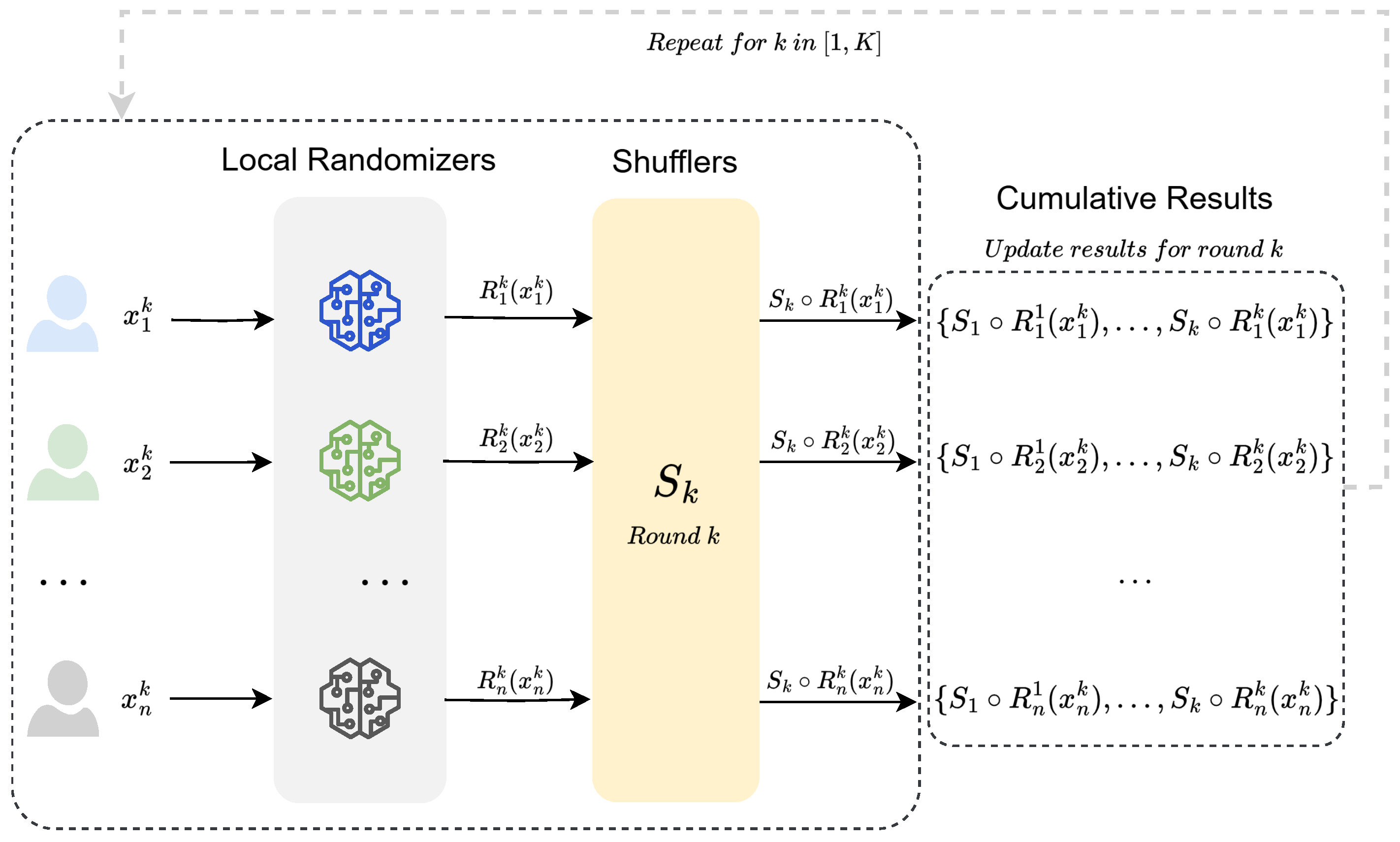
Considering K sequential (and possibly adaptive) queries over a dataset in the shuffle model, there are K rounds of randomization and shuffling, and the shuffling is independent across rounds. Figure 1 provides a detailed visual representation of the K-round shuffle model, highlighting the flow from user input to local randomizers, through shufflers, and finally to the cumulative outputs across K rounds. This complements the mathematical framework described below. Let denote the local randomizers used in the k-th round, where takes the data and the outputs of the previous rounds as input. We use to denote the query result of the k-th round and to denote the outputs during 1 to k rounds:
Assuming that the dominating pair of the k-th round is , that is,
holds for any neighboring datasets and for any distance measure D that satisfy the data processing inequality. Then, using the following lemma from [11] (Theorem 10) and [13] (Corollary 8), we can conclude that the divergence of K-wise sequential composition, , is dominated by
For simplicity, we use to denote variables , and to denote variables .
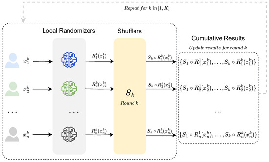
Figure 1.
An overview of the K-round shuffle model, illustrating the randomization and shuffling process in the shuffle model.
Lemma 3
(Reduction of sequential composition [13]). Given any distance measure D that satisfies the data processing inequality, if holds for all and for all neighboring datasets X and , then
Goal of numerical composition of differential privacy for multi-message shuffle protocols. We aim to upper-bound the overall differential privacy consumption of shuffle protocols with K sequential rounds, having broad applications to iterative gradient aggregation in federated learning and various data mining tasks (e.g., building decision tree/forest and a-priori-based frequent itemset mining that compose several sequential steps). Specifically, we analyze the divergence and indistinguishable level of the joint dominating pair:
5. A Tight Characterization of Vector Randomized Response
In this work, we adopt variation–ratio reduction [9] for tightly characterizing a vector randomized response, a prevalent randomizer in shuffle protocols (e.g., in [15,19]). Considering two neighboring datasets X and that differ only in the v-th user’s data (i.e., , , the v-th user is considered as the victim in DP), i.e., and , where . One can define the following properties on (independent) local randomizers with some parameters , , and :
- I.
- -variation property: we say that the -variation property holds if and for all possible .
- II.
- q-ratio property: we say that the q-ratio property holds if and hold for all possible and all .
The parameter represents the pairwise total variation bound of the randomizer , and implies that the randomizer satisfies -LDP. Let denote the sanitized messages of X by , and the variation–ratio analyses [9] reduce the privacy amplification problem into a divergence bound between two binomial counts (see Lemma 4).
Lemma 4
(Variation–ratio reduction [9]). For , let , and and ; let denote and denote . If randomizers satisfy the -variation property and the q-ratio property for all possible that (), then for any measurement D satisfying the data-processing inequality:
Many prevalent multi-message shuffle protocols can be reduced to the dominating pair with varying parameters, including the optimal privacy–utility–communication protocols of [19,28] that are based on randomized response on each bit, the SOTA message–complexity–efficient frequency oracle of [14] based on binary vector randomized response, and the communication efficient frequency oracle of [16,29].
In the protocol of [16,29], the corresponding parameters are obvious, and the variation–ratio reduction is essentially tight (i.e., there are neighboring datasets that reach the dominating pair). Meanwhile, in the vector-randomized-response-based numerical gradient summation protocol [19] designated for federated learning, computing the total variation bound parameter is non-trivial. Specifically, the protocol first samples s dimensions from d dimensions and then sanitizes each dimension using a randomized response. Due to the vast applications of such vector randomized responses in shuffle protocols (also seen in the recursive protocol in [15]), we derive tight total variation bound and a dominating pair for them in Theorem 1.
Theorem 1
(Reduction of Shuffled Sampled Vector Randomized Response Messages). Given a d-dimension binary vector input domain , define a randomized response mechanism that outputs s dimensions with some probability distribution , and for each dimension , outputs the input with probability r (with ), otherwise outputs . Then, for all possible and any measurement D satisfying the data-processing inequality:
with , , and .
Proof.
Recall that the randomizer outputs selected dimensions and sanitized binary values on these dimensions. We denote the output as , where denotes the base randomized response randomizer that flips with probability . Since the dimensions are selected using a public distribution (and are uncorrelated with the input’s value), it is obvious that satisfies -LDP; thus, the p and q parameter are bounded by .
As for the total variation parameter , we firstly consider a fixed value of S. For any possible , the total variation is maximized when and differ at every bit on dimensions S. Without loss of generality, we assume take values of 0s on these dimensions, and take values of 1s on these dimensions. Then, for a output value of , if t have more zeros than ones, . Let k denote the number of zeros in t, we have:
Now enumerating all possible S, we have the total variation bound as:
Finally, utilizing the variation–ratio reduction in Lemma 4, we have the conclusion. □
6. Privacy Loss Distribution of Generalized Dominating Pairs
Generalized dominating pair for shuffle protocols. To cover the more general case and derive numerical composition bounds for various shuffle protocols (e.g., for both single-message and multi-message protocols), the aim of this work is to numerically derive the DP guarantee of the following K-wise composition of the dominating pair as follows:
where and is the binomial variable defined as in Lemma 4 (and also in Theorem 1) with possibly heterogeneous parameters , , , and .
Following the privacy composition methods in [13,27], the privacy loss distribution (PLD) represents the distribution of the logarithm of probability ratios between a dominating pair of distributions. By constructing the PLD, we can use Fast Fourier Transform (FFT) to compose privacy losses and derive the overall privacy consumption.
To approximate the PLD for each round’s shuffle protocol, we consider the generalized binomial counts that tightly dominate many shuffle protocols: , defined as
where
- ,
- ,
- ,
- .
- Here, C represents the number of other users whose outputs are indistinguishable “clones” of the two users, and A denotes the random split between these clones.
The formula of probabilities and their ratios. The PLD measures the distribution of probability ratios. To analyze the probability ratios, we first consider , and . Let , then based on the above sampling process, we have:
Now let , then the ratio of probabilities on point (with ) is given by:
We denote this probability ratio as .
Due to symmetry, the PLDs of and (e.g., these from Lemma 4 or Theorem 1) are the same. Computing the PLD directly involves iterating over a two-dimensional domain of size , which is impractical for large n. Following the approach in [13], we use Hoeffding’s tail bounds for the binomial distributions to limit our computation to regions where the probability mass is significant, neglecting negligible probabilities and adding their total mass to or . By applying Hoeffding’s inequality to both C and A, we focus on subsets and containing most of the mass, reducing the terms to , where is a small tolerance.
Theorem 2.
Given a dominating pair (shorted as ), and define the set
where . For each , define
with . Then, the approximated PLD defined by
where , differs from the true PLD by at most mass τ and contains terms.
Proof.
We apply Hoeffding’s inequality to the binomial random variable . For any , the inequality provides the following bounds:
To ensure that the total probability does not exceed , we impose the condition:
. Solving for v, we obtain
This yields expressions for and . Similarly, we apply Hoeffding’s inequality to to derive expressions for and . The total neglected mass is bounded by .
Next, we estimate the number of terms in . The set contains at most terms. For each i, the set contains at most
terms. Hence, the number of terms in is at most .
Finally, we derive the conclusion by performing the change of variables and . □
In practice, when computing the PLD of , we finitely grid the domain of the PLD (i.e., the values of u) and ensure the neglected mass is below a prescribed tolerance (e.g., ) and add it to . The overall procedure is summarized in Algorithm 1. This approximation significantly reduces computational complexity, and when composing privacy losses, the FFT computation in Lemma 2—dependent only on the number of grid points—becomes the dominant factor.
Comparison with existing accounting approaches. Several works employ the Rényi differential privacy for composition, such as in [8]. However, the Rényi differential privacy is far from tight for the random noises in the shuffle model. The work of [13] proposes numerical composition for LDP randomizers in the shuffle model, though it is applicable to only single-message protocols (corresponding to and in our dominating pair). Commonly used local randomizers (e.g., the vector binary randomized response in [19], see Theorem 1) often have much lower values of total variation bound . Moreover, the single-message protocols are known to have limited utility [12] for common statistical queries (e.g., histogram estimation, numerical vector aggregation), when compared to multi-message shuffle protocols (e.g., in [14,16]).
| Algorithm 1 PLD Computation of | |
| Input: | |
| Output: The PLD of over -grid range with tolerance | |
| 1: | |
| 2: | |
| 3: | |
| 4: | |
| 5: | |
| 6: | |
| 7: | ▷ initializes the PLD with a list of zeros |
| 8: | for to do |
| 9: | |
| 10: | |
| 11: | for to do |
| 12: | |
| 13: | |
| 14: | if and then |
| 15: | |
| 16: | |
| 17: | end if |
| 18: | end for |
| 19: | end for |
| 20: | return |
7. Applications to Federated Learning
7.1. Building Decision Tree/Forest
Decision trees [30] are hierarchical models used for classification and regression tasks, where data are recursively partitioned based on feature values to maximize a purity metric such as information gain or Gini impurity. At each node, the algorithm evaluates possible splits by considering thresholds over features and selects the one that optimally separates the data. Random forests extend this concept by constructing an ensemble of decision trees, each trained on a bootstrap sample of the data and a random subset of features, thereby improving generalization through bagging and feature randomness.
In federated learning settings, where data are distributed across multiple clients with privacy constraints, the traditional centralized approach is infeasible. To address this, the model-building process can be transformed into multiple rounds of histogram estimation. Each client computes local histograms for feature f, aggregating the frequencies of feature values within predefined bins. These set-valued frequency estimations are securely aggregated and sent to a central server, which combines them to approximate the global data distribution: . The server then determines optimal split points based on the aggregated histograms without accessing raw data, enabling the collaborative construction of decision trees and forests while preserving data privacy.
For each histogram frequency query, one can adopt a SOTA shuffle protocol from [14,16,29]. For every one of them, the and parameters can be easily computed (see Section 8 for detail).
7.2. Building Deep Learning Models
Deep learning models, such as neural networks, are powerful tools for learning complex patterns from data. In federated settings, where data are distributed across multiple clients with privacy constraints, training deep learning models requires a collaborative approach that avoids sharing raw data. Federated learning enables this by allowing each client to train a local model on their data and then share model updates (e.g., gradients) with a central server. The server aggregates these updates to improve a global model, iteratively refining it over multiple communication rounds.
To preserve privacy and ensure robustness, the model building process can be transformed into multiple rounds of gradient aggregation with clipping and randomization. After computing local gradients, each client applies gradient clipping to bound the influence of any single update: , where is the local gradient and C is the clipping threshold. Clients then randomize and contribute their clipped gradients using the shuffle model of DP. The central server observes privatized gradients from the shuffler, and then aggregates them to update the global model: . By iterating this process, the federated system collaboratively trains a deep learning model while protecting individual client data.
For each gradient aggregation query, one can adopt the SOTA shuffle protocol for numerical vector summation from [19]. In their protocol, each message is computed from s uniform-randomly selected bits from d dimensions, and each bit is flipped with probability . The corresponding and parameters can be computed using Theorem 1.
7.3. Machine Learning
Many machine learning algorithms naturally align with the multi-round paradigm considered in this work. For example, Isolation Forest for anomaly detection [31] relies on iterative data partitioning to isolate anomalies. This process can be adapted to federated learning using the shuffle model, ensuring privacy during intermediate computations. Similarly, iterative clustering algorithms, such as K-means [32], refine cluster centroids over multiple rounds of aggregation and adjustment. Differential privacy techniques, including the shuffle model, have been shown to effectively protect privacy in these settings. The shuffle model’s privacy amplification effect is particularly beneficial for such iterative computations, enabling secure aggregation of intermediate results like histogram updates or centroid adjustments [6]. This integration extends the applicability of federated learning to tasks such as anomaly detection, clustering, and other iterative machine learning methods in privacy-sensitive scenarios.
8. Experiments
We evaluate the privacy composition results of our proposal on two typical federated learning tasks within the shuffle model: decision trees and deep learning. We simulate shuffle protocols for these learning tasks, and measure their overall privacy consumption. The implementation code is made publicly available at https://github.com/wangsw/PrivacyAmplification/tree/main/sequentialComposition (accessed on 31 January 2025).
8.1. Federated Deep Learning Simulation
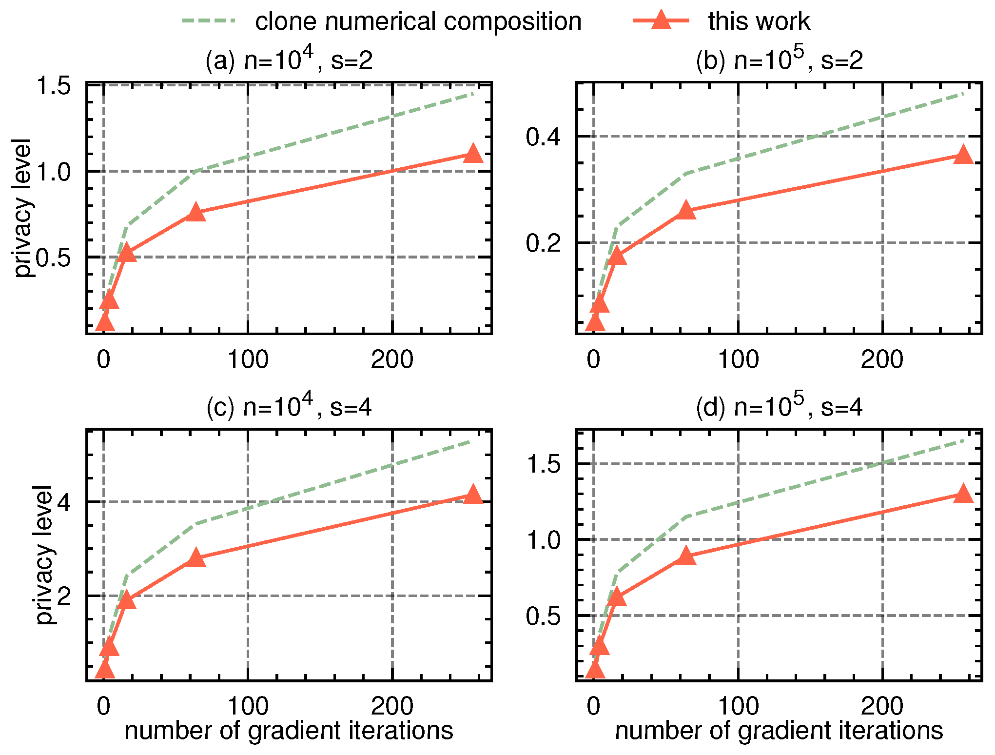
We assume a general deep learning procedure in the shuffle model, where there are K iterative gradient aggregation rounds, and each round collects a gradient vector from n users. Assuming the local budget as , according to optimal numerical vector aggregation protocol [19], each user will send bits in each message. Each bit is sanitized using a randomized response with flipping probability . Overall, the procedure is equivalent to K rounds of shuffle protocols, each using sampled vector -randomized response as the local randomizer with n users. In order to cover extensive scenarios, we vary the number of iterations T from 2 to 256, vary the local budget in , and vary the number of users from to .
The work of [13] for privacy composition of single-message LDP shuffling protocols is applicable to such a scenario, as the sampled vector -randomized response with flipping probability satisfies -LDP. We compare our proposal in Theorem 1 with the numerical approach in [13], which had the tightest so far composition bounds (compared to the Rényi DP-based approaches in [8,10]). We present the experimental results in Figure 2. Since our proposal in Theorem 1 provides a provably tighter dominating pair for vector -randomized response, it consistently reduces about privacy consumption when compared to [13].
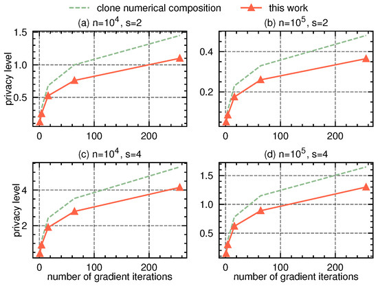
Figure 2.
Privacy accounting comparison in federated deep learning scenarios.
8.2. Federated Decision Tree/Forest Simulation
Recall that decision trees select splitting attributes at each node of the decision tree. At the h-th level (deem the root node as the 0-th level), there are nodes to choose from, each being chosen from candidate attributes. Since each node at the same level is a subpopulation, it is enough to launch histogram queries for all nodes. Therefore, to build a decision with H levels, there are a total of histogram queries. Assuming each attribute has 2 categories, then each histogram query in the h-th level will have categories. We will use the SOTA multi-message histogram estimation protocol of [16] within the shuffle model, where each histogram query will employ the full n-size population. In each histogram protocol in the h-th level, the parameters , , and .
As each round employs the multi-message protocol [16], while [8,13] (which are constrained on single-message protocols) are not applicable, we compare our approach with the basic and advanced privacy composition bound from [3], where each round’s privacy loss is numerically computed using the SOTA variation–ratio reduction [9]. In the histogram estimation protocol, we assume each user contributes m messages: one message for the true category, and messages each as a uniform random category from the domain. Let denote the domain size (number of categories) at the h-th level, and the dominating pair of the protocol has parameters , , . We vary the number of messages per user from 2 to 6, vary the number of users from to , vary the number of tree levels H from 5 to 8, and vary the number of attributes d from 8 to 32.
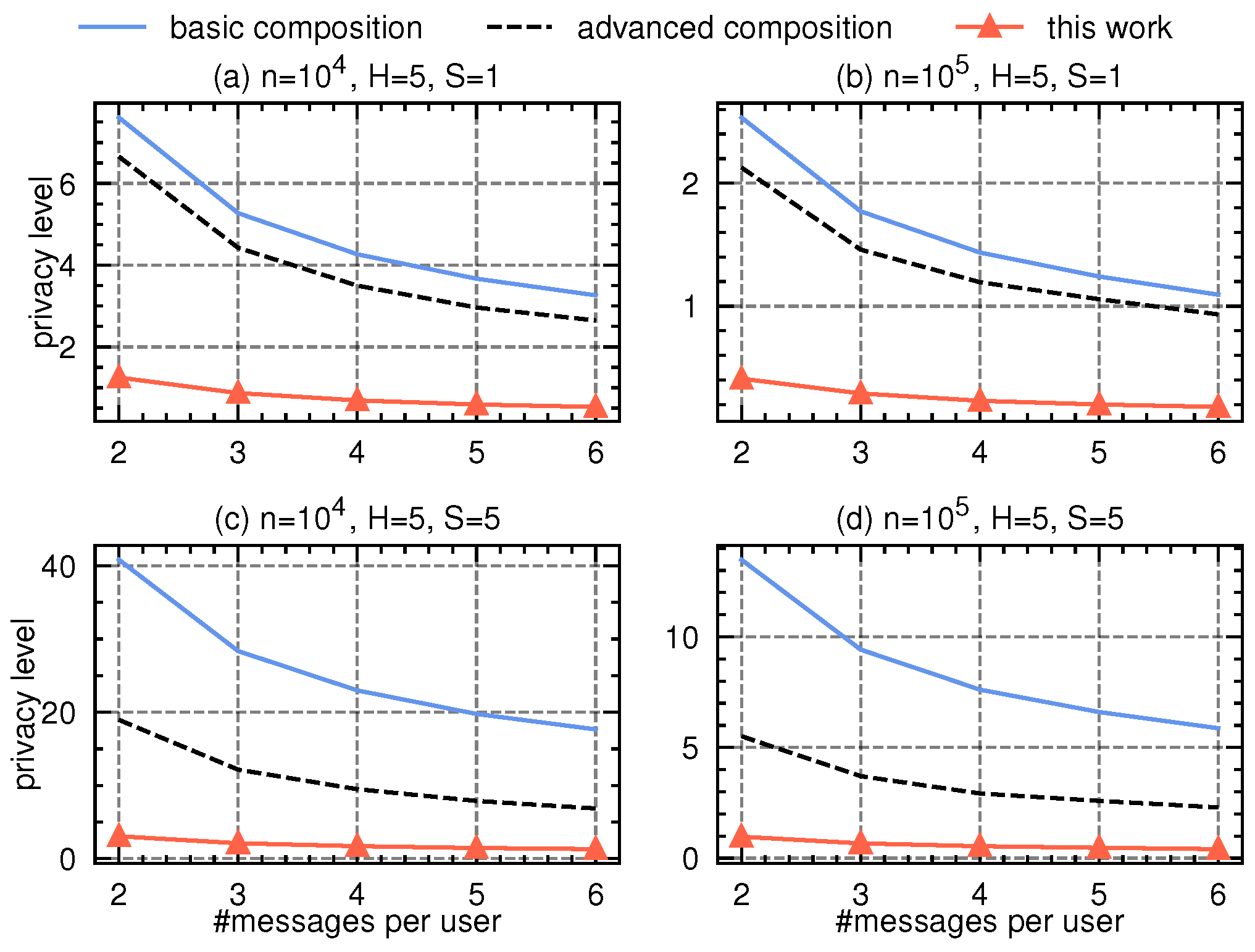
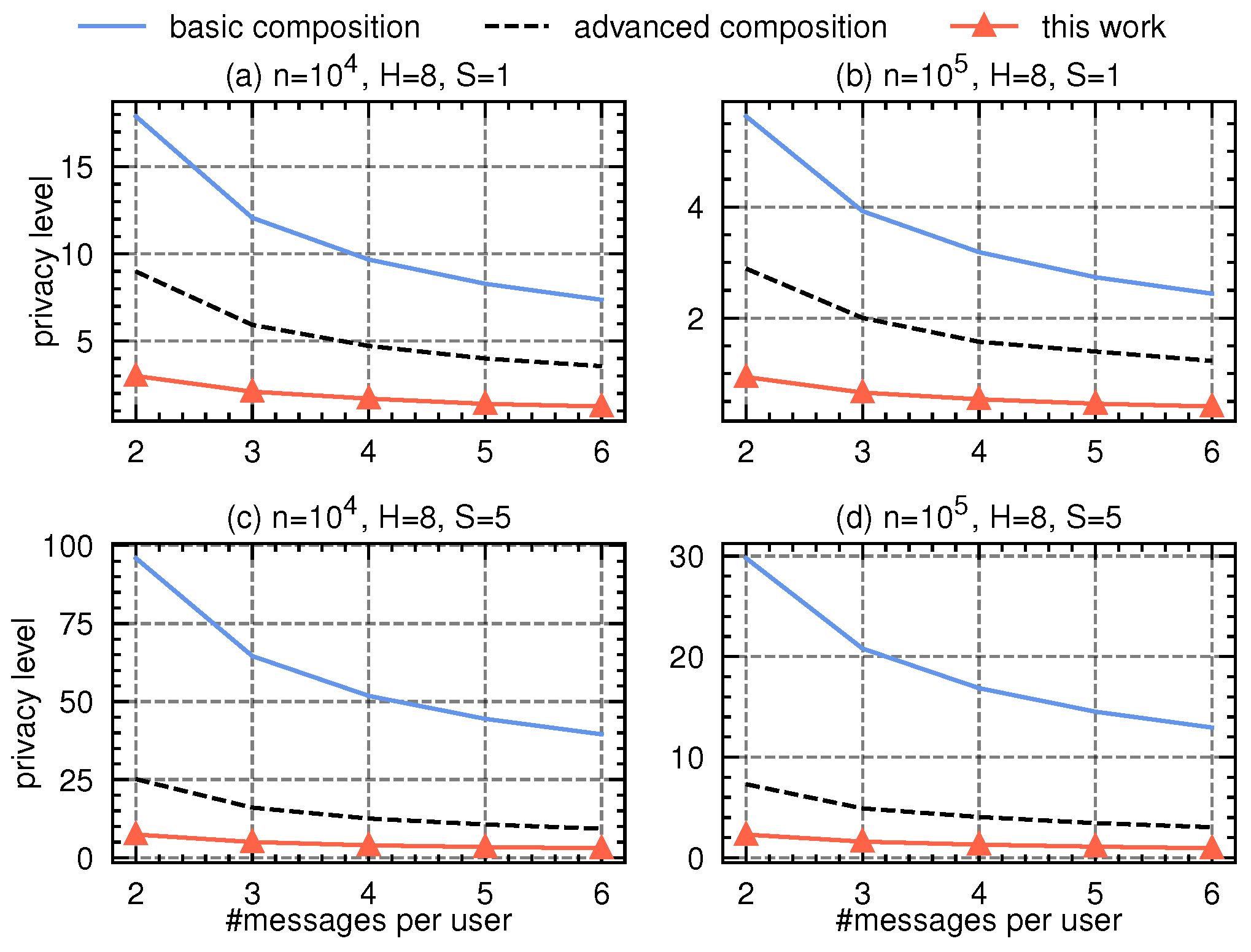
Our proposal is also applicable to decision forest, where multiple decision trees are either created in parallel (e.g., in random forest) or sequentially (e.g., in gradient-boosted decision trees). For illustration, we assume that we build or trees sequentially, covering many practical scenarios. Compared to the single decision tree, decision forest requires more number of privacy compositions. In Figure 3 and Figure 4, we present the experimental results with varying number of messages per user (in the x-axis) and with tree height and , respectively. Compared to basic or advanced composition, our proposal saves remarkably budget.
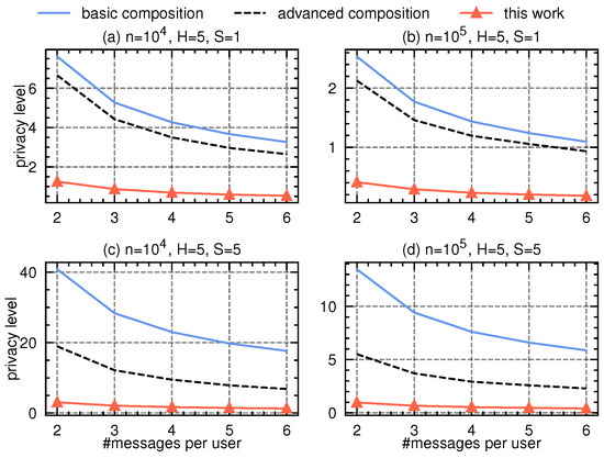
Figure 3.
Privacy accounting comparison in federated decision tree(s) scenarios with tree height .
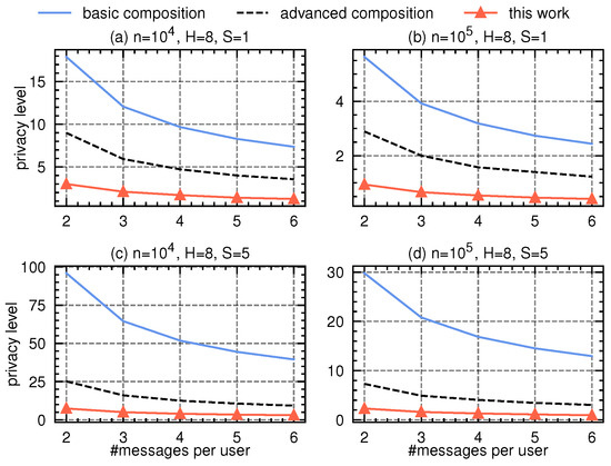
Figure 4.
Privacy accounting comparison in federated decision tree(s) scenarios with tree height .
9. Conclusions
We have presented a numerical composition method for the shuffle model of differential privacy, covering both single-message shuffle protocols and multi-message shuffle protocols, having broad applications to federated analytics and federated learning (e.g., decision tree/forest and deep learning). Specifically, for single-message shuffle protocols that are based on vector randomized response, we provide privacy parameter characterization. For unified dominating pair reduction of single-message/multi-message shuffle protocols, we present an efficient and tight approach for K-wise sequential composition within computational complexity. Through simulations of federated learning in the shuffle model, we show that our proposals save budget for single-message shuffle protocols, and budget for multi-message shuffle protocols.
Nevertheless, several limitations are present in our study. The communication overhead inherent in the shuffling process, particularly in systems with a large number of participants, presents considerable challenges related to scalability and operational efficiency. In the context of a joint learning framework, the additional computational burden imposed by the execution of the shuffling protocol may negatively impact the overall system performance, especially in scenarios characterized by resource limitations or uneven data distribution.
Future Directions: (i) Future research could explore the integration of the shuffle model with complementary privacy-preserving techniques such as homomorphic encryption or secure multi-party computation (SMPC). Such hybrid approaches would enable stronger privacy guarantees for tasks that involve highly sensitive data, such as financial or healthcare data analysis. (ii) Another direction is to investigate the privacy–utility trade-offs in non-numerical tasks, such as text, image, or multimedia analysis, which could expand the shuffle model’s applicability to fields like natural language processing and computer vision.
Author Contributions
Conceptualization, S.W. and J.L.; methodology, S.W. and S.Z.; software, S.W.; validation, J.L., S.H. and Y.C.; formal analysis, S.W.; investigation, S.W. and S.Z.; resources, S.H.; data curation, S.W.; writing—original draft preparation, S.W.; writing—review and editing, S.Z., J.L., S.H. and Y.C.; visualization, S.W. and S.Z.; supervision, S.W.; project administration, S.W. All authors have read and agreed to the published version of the manuscript.
Funding
This work is supported by Guangzhou Basic and Applied Basic Research Foundation (No. 2025A03J3182, No. 202201010194, No. 202201020139).
Institutional Review Board Statement
Not applicable.
Informed Consent Statement
Not applicable.
Data Availability Statement
The raw data supporting the conclusions of this article will be made available by the authors on request.
Conflicts of Interest
The authors declare no conflicts of interest.
References
- Gao, J.; Hou, B.; Guo, X.; Liu, Z.; Zhang, Y.; Chen, K.; Li, J. Secure aggregation is insecure: Category inference attack on federated learning. IEEE Trans. Dependable Secur. Comput. 2021, 20, 147–160. [Google Scholar] [CrossRef]
- Zhu, L.; Liu, Z.; Han, S. Deep leakage from gradients. Adv. Neural Inf. Process. Syst. 2019, 32. [Google Scholar]
- Dwork, C. Differential privacy: A survey of results. In Proceedings of the International Conference on Theory and Applications of Models of Computation, Xi’an, China, 25–29 April 2008; pp. 1–19. [Google Scholar]
- Apple; Google. Exposure Notification Privacy-Preserving Analytics White Paper. 2021. Available online: https://covid19-static.cdn-apple.com/applications/covid19/current/static/contact-tracing/pdf/ENPA_White_Paper.pdf (accessed on 31 January 2025).
- Talwar, K.; Wang, S.; McMillan, A.; Jina, V.; Feldman, V.; Bansal, P.; Basile, B.; Cahill, A.; Chan, Y.S.; Chatzidakis, M.; et al. Samplable anonymous aggregation for private federated data analysis. arXiv 2024, arXiv:2307.15017. [Google Scholar]
- Erlingsson, Ú.; Feldman, V.; Mironov, I.; Raghunathan, A.; Talwar, K.; Thakurta, A. Amplification by shuffling: From local to central differential privacy via anonymity. In Proceedings of the Thirtieth Annual ACM-SIAM Symposium on Discrete Algorithms, San Diego, CA, USA, 6–9 January 2019. [Google Scholar]
- Feldman, V.; McMillan, A.; Talwar, K. Hiding among the clones: A simple and nearly optimal analysis of privacy amplification by shuffling. In Proceedings of the 2021 IEEE 62nd Annual Symposium on Foundations of Computer Science (FOCS), Denver, CO, USA, 7–10 February 2022. [Google Scholar]
- Feldman, V.; McMillan, A.; Talwar, K. Stronger privacy amplification by shuffling for rényi and approximate differential privacy. In Proceedings of the 2023 Annual ACM-SIAM Symposium on Discrete Algorithms (SODA), SIAM, Florence, Italy, 22–25 January 2023. [Google Scholar]
- Wang, S.; Peng, Y.; Li, J.; Wen, Z.; Li, Z.; Yu, S.; Wang, D.; Yang, W. Privacy Amplification via Shuffling: Unified, Simplified, and Tightened. Proc. Vldb Endow. 2024, 17, 1870–1883. [Google Scholar] [CrossRef]
- Girgis, A.; Data, D.; Diggavi, S.; Kairouz, P.; Suresh, A.T. Shuffled model of differential privacy in federated learning. In Proceedings of the 24th International Conference on Artificial Intelligence and Statistics, PMLR, Virtual, 13–15 April 2021. [Google Scholar]
- Zhu, Y.; Dong, J.; Wang, Y.X. Optimal accounting of differential privacy via characteristic function. In Proceedings of the International Conference on Artificial Intelligence and Statistics, PMLR, Virtual, 28–30 March 2022; pp. 4782–4817. [Google Scholar]
- Ghazi, B.; Golowich, N.; Kumar, R.; Pagh, R.; Velingker, A. On the power of multiple anonymous messages: Frequency estimation and selection in the shuffle model of differential privacy. In Proceedings of the Annual International Conference on the Theory and Applications of Cryptographic Techniques, Zagreb, Croatia, 17–21 October 2021; Springer: Cham, Switzerland, 2021; pp. 463–488. [Google Scholar]
- Koskela, A.; Heikkilä, M.A.; Honkela, A. Numerical Accounting in the Shuffle Model of Differential Privacy. Trans. Mach. Learn. Res. 2023. Available online: https://openreview.net/forum?id=11osftjEbF (accessed on 31 January 2025).
- Cheu, A.; Zhilyaev, M. Differentially private histograms in the shuffle model from fake users. In Proceedings of the 2022 IEEE Symposium on Security and Privacy, San Francisco, CA, USA, 22–26 May 2022. [Google Scholar]
- Balle, B.; Bell, J.; Gascon, A.; Nissim, K. Private summation in the multi-message shuffle model. In Proceedings of the 2020 ACM SIGSAC Conference on Computer and Communications Security, Virtual, 9–13 November 2020. [Google Scholar]
- Luo, Q.; Wang, Y.; Yi, K. Frequency Estimation in the Shuffle Model with Almost a Single Message. In Proceedings of the Proceedings of the 2022 ACM SIGSAC Conference on Computer and Communications Security, Los Angeles, CA, USA, 7–11 November 2022; pp. 2219–2232. [Google Scholar]
- Chang, A.; Ghazi, B.; Kumar, R.; Manurangsi, P. Locally private k-means in one round. In Proceedings of the International Conference on Machine Learning, PMLR, Virtual, 18–24 July 2021; pp. 1441–1451. [Google Scholar]
- Tenenbaum, J.; Kaplan, H.; Mansour, Y.; Stemmer, U. Differentially private multi-armed bandits in the shuffle model. In Proceedings of the 35th International Conference on Neural Information Processing Systems, Virtual, 6–14 December 2021. [Google Scholar]
- Girgis, A.M.; Diggavi, S. Multi-message shuffled privacy in federated learning. IEEE J. Sel. Areas Inf. Theory 2024, 5, 12–27. [Google Scholar] [CrossRef]
- Balle, B.; Bell, J.; Gascón, A.; Nissim, K. The privacy blanket of the shuffle model. In Proceedings of the 39th Annual International Cryptology Conference, Santa Barbara, CA, USA, 18–22 August 2019. [Google Scholar]
- Kasiviswanathan, S.P.; Lee, H.K.; Nissim, K.; Raskhodnikova, S.; Smith, A. What can we learn privately? SIAM J. Comput. 2011, 40, 793–826. [Google Scholar] [CrossRef]
- Cheu, A.; Smith, A.; Ullman, J.; Zeber, D.; Zhilyaev, M. Distributed differential privacy via shuffling. In Proceedings of the EUROCRYPT, Darmstadt, Germany, 19–23 May 2019. [Google Scholar]
- Dingledine, R.; Mathewson, N.; Syverson, P. Tor: The Second-Generation Onion Router. In Proceedings of the 13th USENIX Security Symposium (USENIX Security 04), San Diego, CA, USA, 9–13 August 2004. [Google Scholar]
- Bittau, A.; Erlingsson, Ú.; Maniatis, P.; Mironov, I.; Raghunathan, A.; Lie, D.; Rudominer, M.; Kode, U.; Tinnes, J.; Seefeld, B. Prochlo: Strong privacy for analytics in the crowd. In Proceedings of the 26th Symposium on Operating Systems Principles, Shanghai, China, 28 October 2017. [Google Scholar] [CrossRef]
- Xu, S.; Zheng, Y.; Hua, Z. Camel: Communication-Efficient and Maliciously Secure Federated Learning in the Shuffle Model of Differential Privacy. In Proceedings of the 2024 on ACM SIGSAC Conference on Computer and Communications Security, Salt Lake City, UT, USA, 14–18 October 2024; CCS ’24. pp. 243–257. [Google Scholar] [CrossRef]
- Gopi, S.; Lee, Y.T.; Wutschitz, L. Numerical composition of differential privacy. In Proceedings of the Thirty-Fifth Annual Conference on Neural Information Processing Systems, Virtual, 6–14 December 2021. [Google Scholar]
- Koskela, A.; Jälkö, J.; Honkela, A. Computing tight differential privacy guarantees using fft. In Proceedings of the International Conference on Artificial Intelligence and Statistics, PMLR, Online, 26–28 August 2020; pp. 2560–2569. [Google Scholar]
- Chen, W.N.; Song, D.; Ozgur, A.; Kairouz, P. Privacy amplification via compression: Achieving the optimal privacy-accuracy-communication trade-off in distributed mean estimation. Adv. Neural Inf. Process. Syst. 2024, 36, 69202–69227. [Google Scholar]
- Li, X.; Liu, W.; Feng, H.; Huang, K.; Hu, Y.; Liu, J.; Ren, K.; Qin, Z. Privacy enhancement via dummy points in the shuffle model. IEEE Trans. Dependable Secur. Comput. 2023, 21, 1001–1016. [Google Scholar] [CrossRef]
- Rokach, L.; Maimon, O. Decision trees. In Data Mining and Knowledge Discovery Handbook; Springer: New York, NY, USA, 2005; pp. 165–192. [Google Scholar]
- Liu, F.T.; Ting, K.M.; Zhou, Z.H. Isolation forest. In Proceedings of the 2008 Eighth IEEE International Conference on Data Mining, Pisa, Italy, 15–19 December 2008; pp. 413–422. [Google Scholar]
- Krishna, K.; Murty, M.N. Genetic K-means algorithm. IEEE Trans. Syst. Man Cybern. Part B (Cybern.) 1999, 29, 433–439. [Google Scholar] [CrossRef] [PubMed]
Disclaimer/Publisher’s Note: The statements, opinions and data contained in all publications are solely those of the individual author(s) and contributor(s) and not of MDPI and/or the editor(s). MDPI and/or the editor(s) disclaim responsibility for any injury to people or property resulting from any ideas, methods, instructions or products referred to in the content. |
© 2025 by the authors. Licensee MDPI, Basel, Switzerland. This article is an open access article distributed under the terms and conditions of the Creative Commons Attribution (CC BY) license (https://creativecommons.org/licenses/by/4.0/).