An Explainable XGBoost Model for International Roughness Index Prediction and Key Factor Identification

Abstract

This study proposes an explainable extreme gradient boosting (XGBoost) model for predicting the international roughness index (IRI) and identifying the key influencing factors. A comprehensive dataset integrating multiple data sources, such as structure, climate and traffic load, is constructed. A voting-based feature selection strategy is adopted to identify the key influencing factors, which are used as inputs for the prediction model. Multiple machine learning (ML) models are trained to predict the IRI with the constructed dataset, and the XGBoost model performs the best with the coefficient of determination ($R^2$) reaching 0.778. Finally, interpretable techniques including feature importance, Shapley additive explanations (SHAP) and partial dependency plots (PDPs) are employed to reveal the mechanism of influencing factors on IRI. The results demonstrate that climate conditions and traffic load play a critical role in the deterioration of IRI. This study provides a relatively universal perspective for IRI prediction and key factor identification, and the outputs of the proposed method contribute to making scientific maintenance strategies of roads to some extent.

1. Introduction

With the development of transport infrastructure, the mileage of road construction has gradually increased. Under the action of long-term repeated loads, roads will inevitably deteriorate in performance status, threatening the driving safety of vehicles and posing a huge safety risk to transportation [1]. The scientific evaluation of pavement performance and the subsequent rational maintenance decisions are of great practical importance. In the field of pavement performance evaluation, the IRI is usually regarded as the most recognized indicator and has been widely adopted by transport agencies around the world as an indicator for evaluating pavement roughness. As an indicator of pavement roughness, IRI not only measures the condition of the pavement formation but also reflects the ride quality and comfort of road users [2,3]. Therefore, achieving accurate prediction of IRI can help management departments to understand the evolutionary trend of IRI and make scientific maintenance decisions, optimizing resource allocation and improving pavement safety.

Traditional methods, such as statistical correlation analysis [4], the mechanistic-empirical model [5,6,7,8], Markov chains [9,10,11] and the gray relation model [12,13,14], are used to predict pavement deterioration. However, these methods have limited abilities to utilize complex pavement information. Under such circumstances, machine learning (ML)-based models have been widely adopted to predict pavement performance. Support vector machines (SVMs), decision trees and Gaussian process regression (GPR) are presented as basic ML algorithms for pavement roughness prediction. Wang et al. [15] developed a hybrid gray relation analysis (GRA) and support vector machine regression (SVR) technique to predict pavement performance. Linear regression, optimized trees and optimized GPR are used for predicting IRI [16]. Qiao et al. [17] employed the least absolute shrinkage and selection operator (Lasso) and ridge regression, SVR and regression trees to estimate reliable IRI.

Recently, ensemble learning methods have offered enhanced capabilities of processing high-dimensional data, effectively solving nonlinear problems. The random forest (RF) algorithm has been extensively employed as a robust approach for IRI prediction [18,19]. Guo et al. [20] constructed an RF model to fit the principles for the potential deterioration of the typical flexible pavement. Gong et al. [18] developed a random forest regression (RFR) model and found that the initial IRI is the most important factor influencing the development of IRI. At the same time, they observed that cracks, ruts, average annual precipitation and service life also have significant impacts on IRI. In addition, the emergence of boosting ensemble learning methods, including gradient boosting decision trees (GBDTs) and XGBoost, has further improved the nonlinear processing capabilities of ML models. Based on XGBoost, Luo et al. [21] evaluated the effectiveness of four preventive maintenance treatments on asphalt pavement roughness and revealed that the annual average traffic volume contributed the most to IRI, followed by precipitation, rut depth and temperature. Damirchilo et al. [22] also developed an XGBoost model for IRI prediction and found that hydraulic conductivity and the average of equivalent single-axle loads have marked impacts on IRI. El-Hakim et al. [23] conducted a study for IRI prediction of continuous reinforced concrete pavements and showed that the initial IRI value was the most critical factor, followed by site coefficients, the number of transverse cracks and pavement repairs. Overall, ML algorithms can be used to improve model prediction accuracy. An AdaBoost regression (ABR) model was developed to improve the prediction ability of IRI, with an $R^2$ value of 0.9751 [24].

Although ML models exhibit great computational performance, their typically shallow structures limit their predictive capabilities. Deep learning (DL) algorithms possess strong multi-dimensional data extraction capabilities, enabling them to effectively capture nonlinear relationships within data and exhibit excellent predictive capabilities. Artificial neural networks (ANNs), as a representative of deep learning (DL), are a common tool for building pavement performance prediction models of flexible and rigid pavements [25,26]. Based on the data extracted from the long-term pavement performance (LTPP) database, Zeiada et al. [27] used an ANN-driven forward sequential feature selection algorithm to identify the most important design factors in warm climate regions. By taking the average annual temperature, freezing index, maximum humidity and so on as input parameters, Hossain et al. [28] developed a prediction model for IRI using ANNs for flexible pavements located in wet-freeze, dry-freeze, wet no-freeze and dry no-freeze zones. Based on an adaptive network-based fuzzy inference system (ANFIS) and various meta-heuristic optimizations including the genetic algorithm (GA) and particle swarm optimization (PSO), Nguyen et al. [29] proposed a new hybrid algorithm for IRI prediction and demonstrated the superiority of PSO-based algorithms to other algorithms for evaluating the quality of pavement roughness.

Based on the analysis of the above research, the limitations of IRI prediction can be summarized as follows. Firstly, the study of pavement roughness is limited by the difficulty of acquiring and integrating data from multiple sources. Acquiring and integrating these data is challenging. Secondly, the factors influencing IRI are diverse and complicated. Most existing prediction models fail to identify the key factors. Including all variables from the dataset as inputs into the prediction model can lead to significant reductions in both computational efficiency and model accuracy. Third, ML models, especially ensemble learning and DL, are often referred to as ‘black boxes’. Because their complex internal structures limit direct interpretability, it is difficult to directly explain the influence mechanisms of key factors on IRI. When the physical models are well defined and based on a solid mechanistic understanding, they are preferred. However, ML methods are particularly useful when the problem is nonlinear and complex and where physical models are either incomplete or computationally expensive.

To address these issues, we compiled a pavement roughness dataset for the period 1989–2018 from the LTPP database. By achieving spatial and temporal alignment using the annual intervals as the temporal scale and the state code and unique identifiers as spatial references, this study developed a high-quality, multi-source dataset. Multicollinearity in the multi-source dataset was handled by the variance inflation factor (VIF). Subsequently, feature selection was performed to identify the key influencing factors of IRI using a voting strategy. On this basis, we proposed a novel IRI prediction model based on XGBoost and compared it with the RF and GBDT models. Finally, we utilized the interpretable methods to reveal the mechanism of the key factors. The main contributions of this study are as follows:

(1)

In this study, a spatial-temporally aligned multi-source pavement roughness dataset is constructed. By integrating sample data on pavement structure, climate conditions, traffic load and pavement performance, the dataset provides a comprehensive basis for analysis. To identify the key factors influencing the IRI, a feature selection framework is developed that combines the mutual information method, the random forest–recursive feature elimination (RF-RFE) algorithm, the Lasso regression method and a voting-based strategy.

(2)

Based on the identified key factors, an IRI prediction model based on XGBoost is developed. Comparative analysis such as the mean absolute error ($MAE$), the mean absolute percentage error ($MAPE$), the root mean square error ($RMSE$), the coefficient of determination ($R^2$) and the comparison of actual and predicted IRI show that the XGBoost-based model achieves superior prediction performance.

(3)

This study further reveals the mechanism of each key influencing factor on pavement roughness by employing interpretable techniques, including feature importance, SHAP and PDP. This work addresses a critical gap in the existing literature by providing the mechanism analysis of the causal and contributory roles of these factors, addressing a critical gap in the existing literature by elucidating the mechanisms of pavement performance deterioration.

The remainder of this paper is organized as follows. Section 2 introduces the construction of a comprehensive multi-source dataset for pavement roughness using the LTPP database to integrate information on pavement structure, climate, traffic and pavement performance. Section 3 presents the prediction methods and interpretable methods employed in this research, including RF, GBDT, XGBoost, feature importance, SHAP and PDP. Section 4 discusses the results and analysis of different prediction models, highlighting the comparison of model performance and the mechanism analysis of identified key factors. Section 5 summarizes the conclusion and presents the future work.

2. Materials

2.1. Data Sources

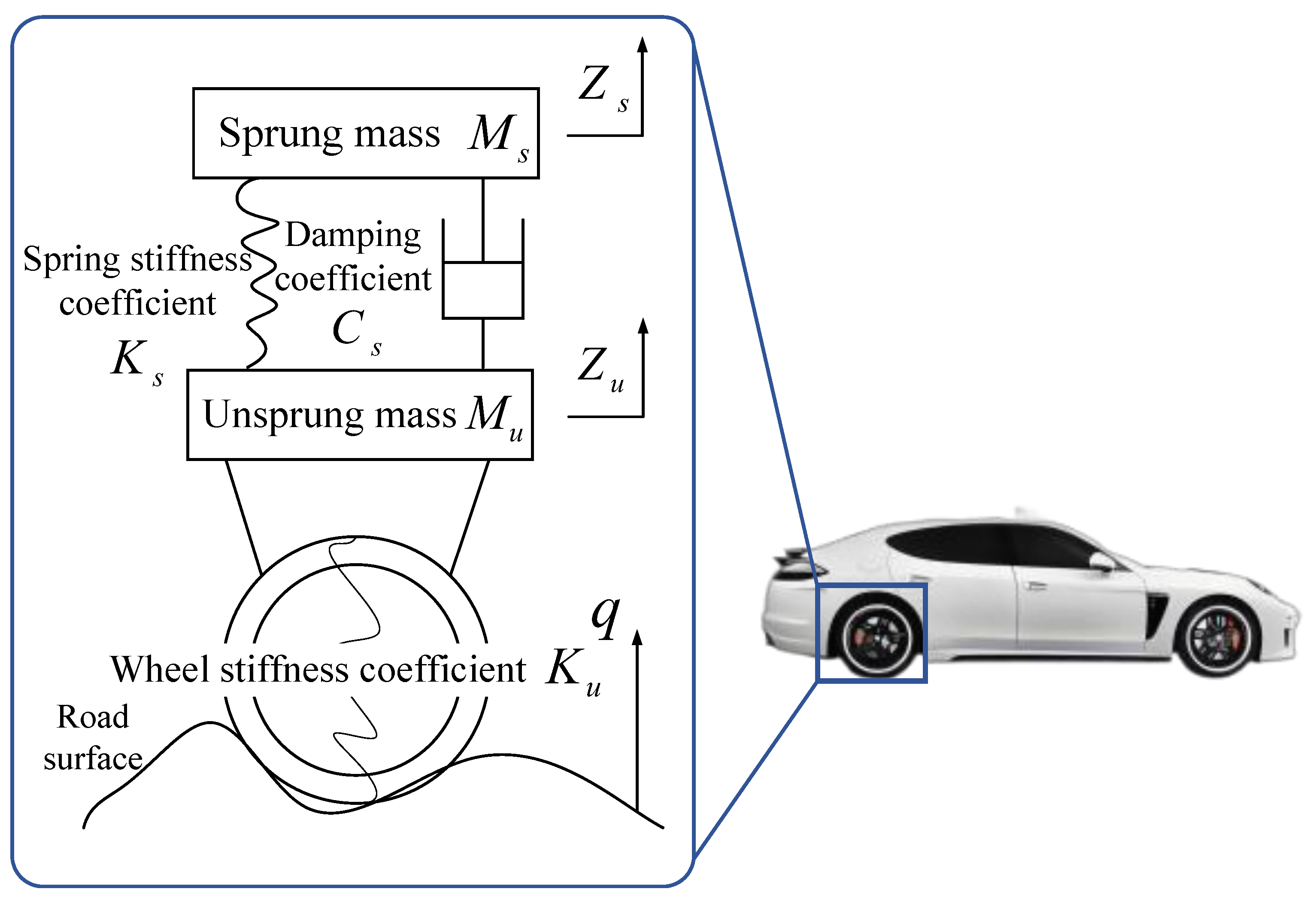
Pavement roughness is predominantly gauged by detecting changes in vibration amplitude when a vehicle passes over the surface. As shown in Figure 1, IRI is developed through a quarter car model, which represents the response of a single tire on the suspension of a vehicle to pavement roughness while running at a speed of 80 km/h [30]. The IRI is expressed in units of m/km, and the formula for calculating IRI is given by [31,32]

$$IRI=a+b\times BI$$

(1)

where detailed variable definitions are provided in Table A3 in Appendix A. Higher IRI values indicate poor roughness and reduced driving comfort.

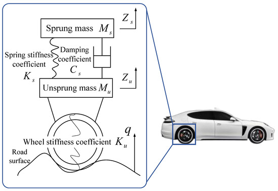
Figure 1. Quarter car model.

2.2. Data Extraction

Relevant studies have taken pavement structure, climate and traffic as influencing factors to study pavement roughness, as shown in Figure 2. The data used in this study were obtained from the LTPP database, which is publicly available through the LTPP office website at https://infopave.fhwa.dot.gov/Data/DataSelection, (accessed on 12 February 2024) [33]. Using the ACCESS tool (Microsoft Access 16.0), this study constructed a spatial-temporally aligned multi-source dataset for pavement roughness. The selection of influencing factors for this study are shown as follows:

(1)

Pavement structure properties. Variables including total asphalt, thickness and total pavement thickness have been well recognized as critical factors affecting the pavement performance [34]. Structural number, layer thickness and subgrade modulus are adopted to represent the pavement structure properties [35]. Therefore, this paper introduces the pavement material type and thickness as input variables. The refined pavement structure factors enable the model to fully consider the effect of material differences on pavement roughness.

(2)

Traffic volume. Traffic volume, climate and service age have significant impacts on performance [36]. The number of actions of the equivalent standard axle load (ESAL) is used to represent the traffic loads. This variable is able to quantify the cumulative effect of traffic loads on pavement damage more accurately, capturing the pavement roughness degradation due to traffic loads.

(3)

Climatic conditions. Climate is considered in prediction models in [24,37]. This study not only includes conventional indicators such as temperature, humidity and precipitation but also considers the number of freeze–thaw cycles as well as shortwave radiation. The complex effects of climatic conditions on pavement roughness are systematically analyzed through a multi-dimensional combination of climatic factors.

(4)

Performance data. This study extracts pavement performance data corresponding to the latest IRI in the LTPP database. This study does not incorporate temporal continuity into the prediction model because the available IRI data are collected on an annual basis rather than shorter, continuous time intervals. Instead, the average of the left and right wheel path IRI values (mean roughness index) over the last five years was used as the IRI value. This approach provides a stable representation of pavement performance while mitigating the impact of single-year anomalies.

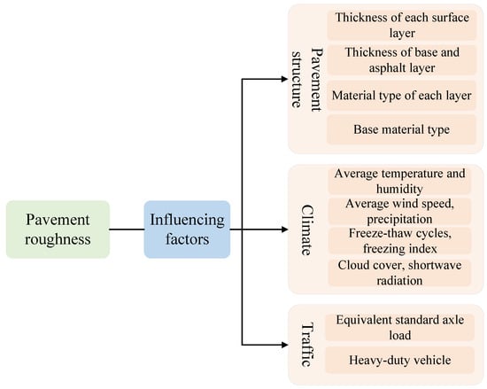
Figure 2. Influencing factors of pavement roughness.

Figure 2. Influencing factors of pavement roughness.

This study initially selected 14 independent variables for predicting IRI. The dependent variable was the average IRI value of the left and right wheel tracks. Table 1 presents the details of these variables. The ‘Source LTPP data sheet’ in Table 1 provides the relevant table names corresponding to the variables in the dataset. To replicate the data extraction process, users can navigate to the Standard Data Release 38 (SDR38) and follow the table names to extract pavement information. A detailed description of the variables listed in Table 1, including the ranges of continuous variables and the numerical encoding of categorical variables, is provided in Table A1 and Table A2 in Appendix A.

Table 1. Description and source of features.

Feature Name	Description	Source LTPP Data Sheet
MAINTENANCE	Road section repair and maintenance times	TST_L05B
GB_THICKNESS	Average thickness of unbonded (granular) base (GB)	TST_L05B
SUBGRADE_MATL	Base material code	TST_L05B
AC_THICKNESS	Average thickness of asphalt concrete layer (AC)	TST_L05B
DRAINAGE_TYPE	Type of underground drainage	SECTION_DRAINAGE_TYPE
PRECIPITATION	Annual precipitation	MERRA_PRECIP_YEAR
TEMP	Annual average temperature	MERRA_TEMP_YEAR
FREEZE_INDEX	Freezing index	MERRA_TEMP_YEAR
FREEZE_THAW	Number of freeze–thaw cycles	MERRA_TEMP_YEAR
WIND	Wind speed	MERRA_WIND_YEAR
HUMIDITY	Mean annual humidity	MERRA_HUMID_YEAR
CLOUD_COVER	Average hourly cloud coverage	MERRA_HUMID_YEAR
SHORTWAVE_SURFACE	Mean duration of surface incident shortwave radiation	MERRA_SOLAR_YEAR
ESAL	The equivalent number of actions of a standard axle load	TRF_TREND
MRI	Average IRI values of left and right wheel tracks	ANALYSIS_IRI

2.3. Data Processing

The set of techniques used prior to the application of a data mining method is named data preprocessing for data mining [38]. Efficient data preprocessing is essential to ensure the quality and reliability of the input data used in predictive modeling. In this study, a systematic approach was adopted, including outlier detection and the handling of outlier and missing values, as detailed below:

(1)

For continuous variables, the interquartile range (IQR) method was applied to detect outliers. The $IQR$ is based on the quartile and the interquartile range; the outliers refer to values less than $Q_L-1.5IQR$ or greater than $Q_U+1.5IQR$, where $Q_L$ is the lower quartile and $Q_U$ is the upper quartile [39].

(2)

After detecting the outliers, anomalous data in a particular column of data can be repaired by interpolation using the average of their neighboring values or data values that have a high correlation with them [32].

(3)

The categorical variable of subgrade material was recoded due to excessive categorization in the type of subgrade material (SUBGRADE_MATL_CODE), as shown in Table 2.

Table 2. The principle of recoding.

Classified Variable	Original Sort Code	Code
SUBGRADE_MATL	101–148	1 (fine-grained soil)
	202–207, 252–257	2 (poorly graded coarse-grained soil)
	201, 209–217, 259–267	3 (well-graded coarse-grained soil)
	282, 287	4 (rock)
DRAINAGE_TYPE	1	1 (no underground drainage)
	2–7	2 (underground drainage)

2.4. Multicollinearity Processing

In regression analysis, there is a high correlation between multiple independent variables, that is, multicollinearity, which leads to instability in model estimates and a decline in predictive effectiveness. The VIF is a common method to detect multicollinearity. The classical linear regression model is expressed as:

$$Y={\beta }_0+{\beta }_1{X}_1+{\beta }_2{X}_2+...+{\beta }_k{X}_k+ϵ$$

(2)

where detailed variable definitions are provided in Table A3 in Appendix A.

For each independent variable $X_i$, the VIF value is calculated as follows:

$$VI{F}_i={\displaystyle \frac{1}{1-R_i^2}}$$

(3)

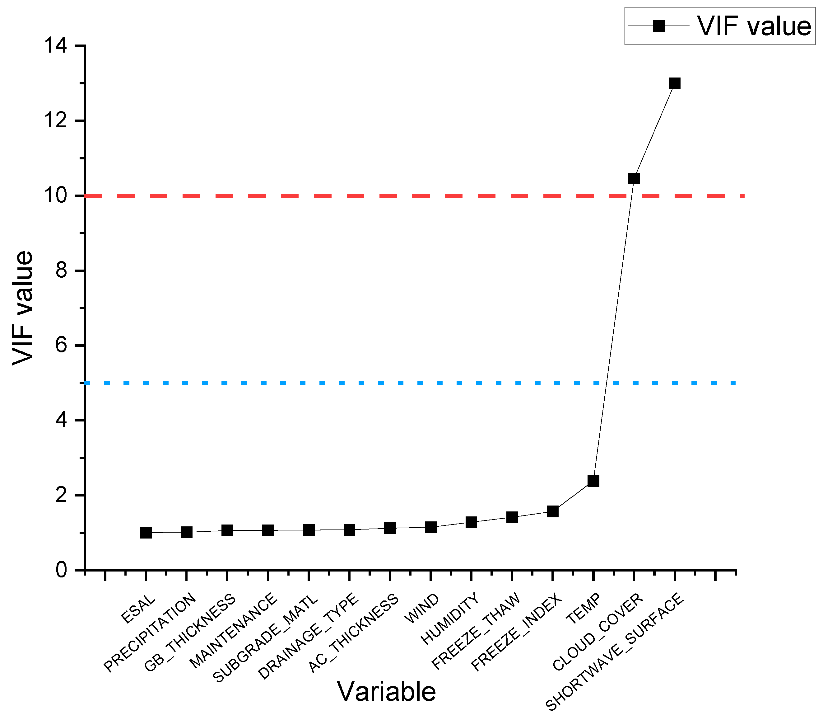
where $R_i^2$ is the coefficient of determination between the i influence factor and the other influence factors. The larger $VI{F}_i$ is, the larger the $R_i^2$ is, indicating that the fit is better and the degree of collinearity between the i explanatory variable and the other explanatory variables is higher. It is generally believed that when $VIF>5$, there is an obvious collinearity problem between the i explanatory variable and other explanatory variables, and when $VIF\ge 10$, it means that there is a serious multicollinearity between the explanatory variables. The VIF values of the independent variables are shown in Figure 3.

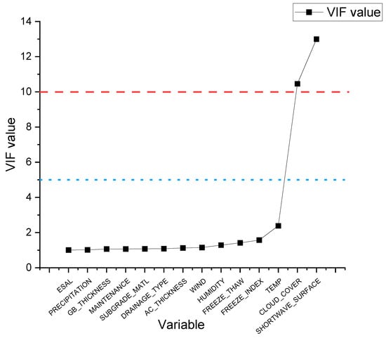
Figure 3. VIF values.

As can be seen in Figure 3, the VIF values of the variables CLOUD_COVER and SHORTWAVE_SURFACE in the dataset of this study are greater than 10, indicating a serious multicollinearity problem. CLOUD_COVER significantly influences the amount of solar shortwave radiation reaching the surface, where high cloud cover reduces shortwave radiation, thus creating a strong correlation between these two variables. To solve the problem of multicollinearity, the variable SHORTWAVE_SURFACE with a high VIF value was first removed, and the VIF value was recalculated. The new VIF values are shown in Table 3. After removing SHORTWAVE_SURFACE, the multicollinearity problem was sufficiently mitigated, as the VIF value of CLOUD_COVER dropped below the threshold of 10. This reduction occurred because the primary source of its multicollinearity was eliminated, reducing the $R^2$ value when regressing CLOUD_COVER on the remaining variables. The number of independent variables in the dataset after multicollinearity treatment is 13.

Table 3. New VIF values.

Variable	VIF	Variable	VIF
PRECIPITATION	1.018	MAINTENANCE	1.071
TEMP	1.216	GB_THICKNESS	1.047
FREEZE_INDEX	1.567	SUBGRADE_MATL	1.042
FREEZE_THAW	1.423	AC_THICKNESS	1.049
WIND	1.152	DRAINAGE_TYPE	1.082
HUMIDITY	1.285	ESAL	1.011
CLOUD_COVER	1.274

In this study, the retained variables after the multicollinearity processing are used as independent variables, and the average of the left and right wheel track IRI values are used as independent variables, which represent the pavement roughness.

3. Methods

3.1. Feature Selection

The objective of feature selection is to identify the most optimal subset of features, comprising only those that are relevant and non-redundant. Feature selection methods have been used to reduce the complexity of datasets in fields such as agriculture, finance and information [40,41]. In this study, a voting-based feature selection strategy was adopted to identify the key influencing factors, which integrates results from the mutual information method, RF-RFE and Lasso regression.

Specifically, the principles of each method are as follows. Mutual information measures the dependency between features and target variables [42]. Although the method is computationally efficient, it may not handle feature redundancy well and could lead to model overfitting. RF-RFE gradually eliminates less important features based on the feature importance derived from the RF model [43]. It continues until the number of features reaches a predetermined threshold or until no further improvements in model performance are observed. While RF-RFE is more accurate in feature selection, it is computationally more intensive. Lasso regression applies an L1 regularization term, which penalizes large coefficients, forcing some coefficients to zero [44]. This helps with feature selection and prevents overfitting, but it may oversimplify the model, possibly discarding important features.

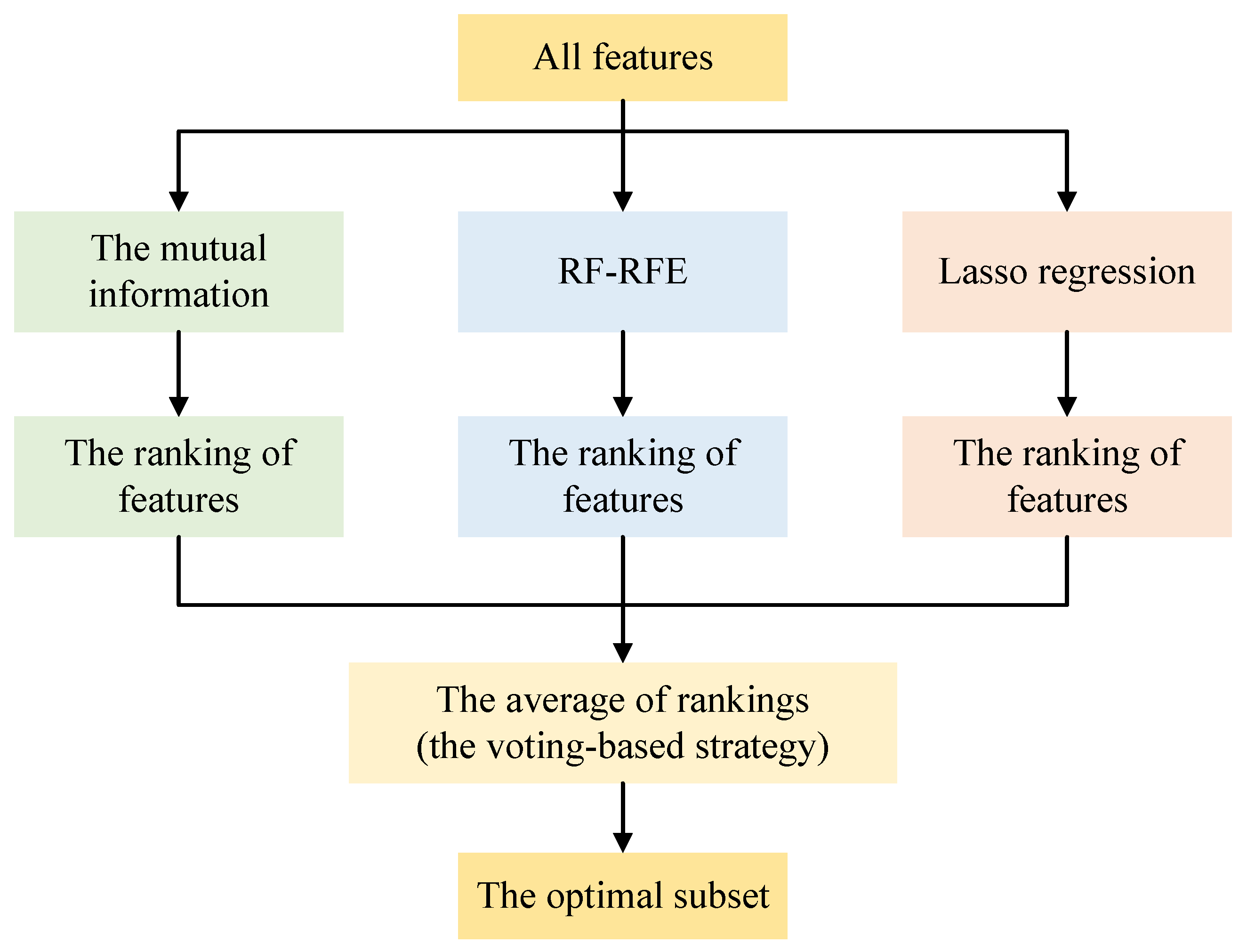
The voting-based feature selection process is illustrated in Figure 4. For each feature, a ranking was generated by these three methods, and a final score was calculated by averaging the rankings. Features with the lowest average rankings were selected as the optimal subset, ensuring a more robust and comprehensive feature selection outcome. This voting strategy mitigates potential biases of any single method, offering a more balanced assessment of the feature contributions and reducing the likelihood of selecting irrelevant features.

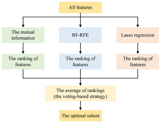
Figure 4. The process of the voting-based feature selection strategy.

3.2. ML Algorithms

3.2.1. Model Selection

Different algorithms have different strengths and adaptations, making model selection crucial for improving prediction performance. In this study, ML algorithms such as RF, GBDT and XGBoost are selected for the prediction of IRI. The reasons for selecting these three models are as follows.

(1)

The primary objective of this study is to accurately predict pavement performance, which is a regression problem with complex nonlinear relationships among pavement structures, traffic loads and climate conditions. Therefore, the selected models are suitable to handle nonlinear data and multivariate interactions.

(2)

Tree-based ensemble methods are particularly suitable for this study as they naturally capture nonlinearity while providing feature importance for further interpretability. Specifically, RF is recognized for its robustness to noise and relatively lower risk of overfitting. The GBDT model makes it powerful for capturing complex data patterns. XGBoost has demonstrated superior performance in predictive tasks with large datasets, which is an enhanced version of the GBDT with regularization.

(3)

Compared to MLR or support vector regression (SVR), the chosen models offer a balance between empirical performance and interpretability. Tools such as SHAP and PDPs enhance the understanding of the impact of key variables on pavement roughness, allowing for a more comprehensive analysis of influencing factors.

This combination of performance, robustness and interpretability justifies the selection of these models for the task. References further corroborate the suitability of these approaches for similar predictive modeling problems.

3.2.2. Random Forest (RF)

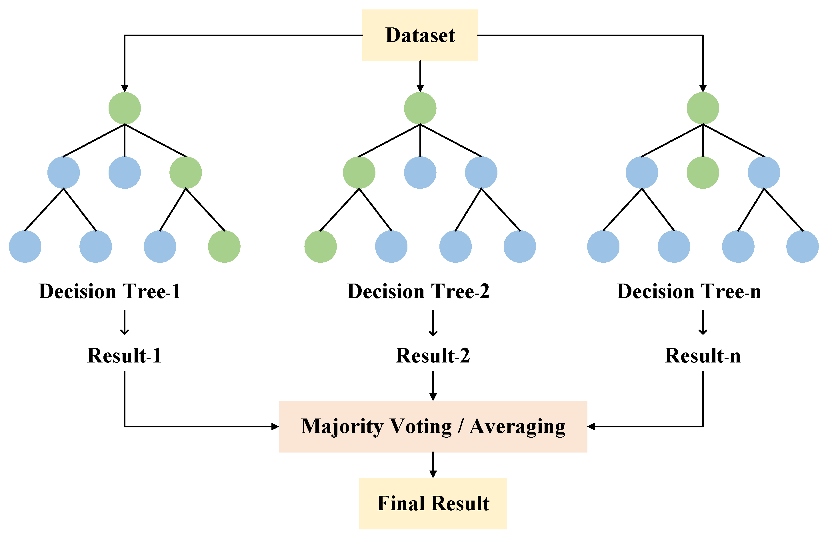
RF is an ensemble ML algorithm based on decision trees, introduced by Breiman [45]. RF uses bootstrap sampling, where each decision tree is trained on randomly selected samples from the original training dataset with replacement. At each split in a decision tree, a random subset of input features is selected, and the best split is determined based on a random subset of the features. The final prediction of RF is obtained by aggregating the predictions of each decision tree predictor. For classification tasks, the RF determines the final prediction using majority voting across all trees. For regression tasks, the final prediction is the mean of the predictions from all trees. Figure 5 shows the principle of RF. The critical parameters of the RF model, which require tuning to optimize performance, are summarized in Table 4.

Figure 5. The principle of RF.

Table 4. RF model parameters.

Parameter	Meaning of Parameter
n_estimators	The number of decision trees in the forest.
max_depth	The maximum depth of each decision tree, controlling model complexity.
min_samples_split	The minimum number of samples that can be divided into leaf nodes; the default value is 2.
min_samples_leaf	The minimum sample size that a leaf node must contain, with a default value of 1.
max_features	The maximum number of features used for each split.
bootstrap	A Boolean indicating whether bootstrap sampling is used when building trees, and the default is true.

3.2.3. Gradient Boosting Decision Tree (GBDT)

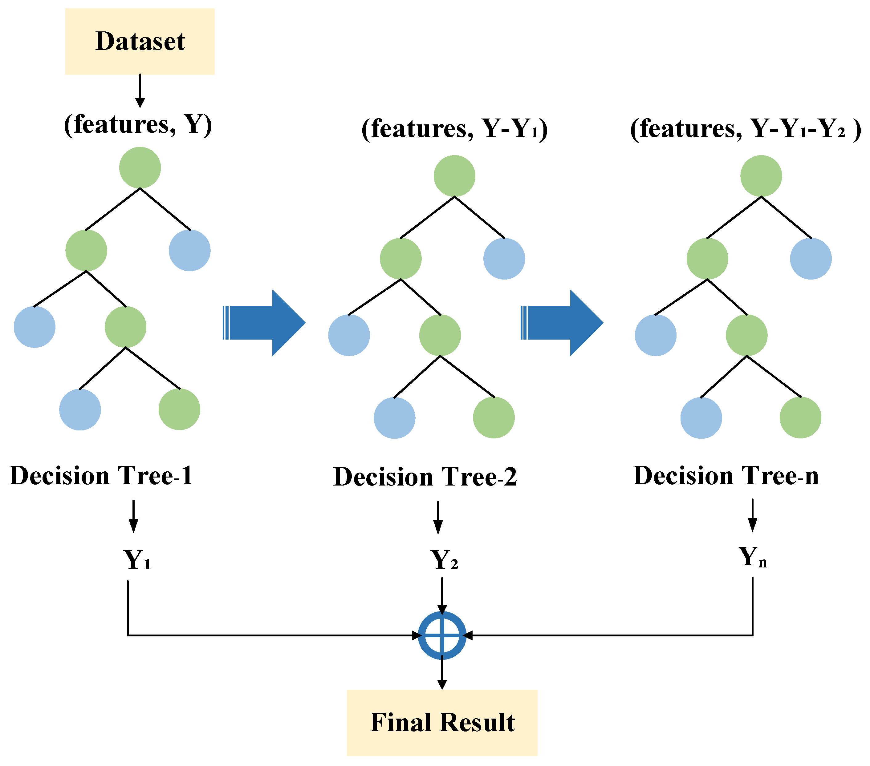
The GBDT is a powerful boosting algorithm, which builds a series of decision trees as weak learners. The main idea of gradient boosting is to construct each decision tree model sequentially in the gradient descent direction of the loss function based on the residuals of the previous model so that the loss of each iteration decreases along the negative gradient, and the prediction is determined based on the sum of the results of all decision trees [46]. The principle of the GBDT is shown in Figure 6. The framework of the GBDT is described as follows [47].

Figure 6. The principle of the GBDT.

Let $D=\left\{\left(x_i,y_i\right)\mid i\in \{1,\dots ,n\},x_i\in R^m,y_i\in R\right\}$ denote the dataset. The basic learner is $h\left(x\right)$, $x_i=(x_{1i},x_{2i},...,x_{pi})$ is the eigenvector, and p is the number of features. $y_i$ is the predicted value, and n denotes the number of samples for training. The steps of the GBDT [47,48] are presented as follows:

(1)

For regression tasks, the initial predicted value is obtained by calculating the average of all samples, which serves as the basis for subsequent iterations. The initial constant value of the model $F_0\left(x\right)$ is given:

$$F_0\left(x\right)={\displaystyle \frac{1}{n}}\sum _{i=1}^n{y}_i$$

(4)

(2)

For the number of iterations $m\in \{1,\dots ,M\}$, M is the times of iteration. The residuals of the ($m-1$)th iteration of the model with respect to $y_i$ are calculated. Residuals reflect the parts of the current model that have not yet been fitted, and subsequent models are fitted by constructing decision trees for these residuals.

$$r_i^{\left(m\right)}=y_i-F_{m-1}\left(x_i\right)$$

(5)

(3)

The basic learner is used to fit a regression tree $h_m\left(x_i\right)$ with $(x_i,r_i^{\left(m\right)})$ as the new training data. The construction of a regression tree is achieved through the split of the feature space, ensuring that the data within each leaf node exhibit comparable objective values.

(4)

The mth iteration model $F_m\left(x\right)$ is updated.

$$F_m\left(x\right)=F_{m-1}\left(x\right)+{\alpha }_m{h}_m\left(x_i\right)$$

(6)

where ${\alpha }_m$ denotes the learning rate, which is defined as the extent to which each newly generated decision tree influences the final predicted value.

(5)

Following M iterations, the final model $F_M\left(x\right)$ is obtained.

$$F_M\left(x\right)=F_0\left(x\right)+\sum _{m=1}^M{\alpha }_m{h}_m\left(x_i\right)$$

(7)

The performance of the GBDT is affected by hyperparameters, and reasonable adjustment of these parameters can improve the predictive accuracy of the model. The meaning of the parameters that need to be tuned in the GBDT model is shown in Table 5.

Table 5. GBDT model parameters.

Parameter	Meaning of Parameter
n_estimators	The number of weak learners (decision trees) to be built.
max_depth	The maximum depth of each tree.
min_samples_split	The minimum number of samples that can be divided into leaf nodes; the default value is 2.
min_samples_leaf	The minimum sample size that a leaf node contains, with a default value of 1.
max_features	The maximum number of features used by a single decision tree; default value none (all features).
learning_rate	Learning rate.
subsample	The fraction of samples to be used for fitting each base learner. Default is 1.0, and values less than 1.0 introduce randomness, which can reduce overfitting.

3.2.4. Extreme Gradient Boosting (XGBoost)

XGBoost is an iterative tree algorithm based on decision trees, developed by Chen and Guestin [49]. XGBoost introduces Lasso and ridge regularization and is a more efficient and flexible gradient boosting algorithm. The framework of XGBoost is described as follows.

Suppose that for a given dataset $D=\left\{\left(x_i,y_i\right)\mid i\in \{1,\dots ,n\},x_i\in R^m,y_i\in R\right\}$, $x_i=(x_{1i},x_{2i},...,x_{mi})$, there are n samples with m features.

The objective function comprises two parts: the first part is termed a training loss, and the second part is termed a regularization.

$$Obj=\sum _{i=1}^{n}L\left(y_i,{\widehat{y}}_i^k\right)+\mathsf{\Omega }\left(f_k\right)+c$$

(8)

where $L\left(y_i,{\widehat{y}}_i^k\right)$ denotes the loss function, which indicates the difference between $y_i$ and ${\widehat{y}}_i$, $y_i$ denotes the true value and ${\widehat{y}}_i^k$ denotes the predicted value of the sample at the kth iteration. $\mathsf{\Omega }\left(f_k\right)$ represents the regularization, and c is constant. $\mathsf{\Omega }\left(f_k\right)$ is given as:

$$\mathsf{\Omega }\left(f_k\right)=\gamma T+{\displaystyle \frac{1}{2}}\lambda \sum _{k=1}^K{w}_j^2$$

(9)

where $\gamma$ and $\lambda$ denote the penalty terms to avoid overfitting. T represents the total number of nodes, j denotes the number of nodes in each of the tth trees, and $w_j$ is the optimization objective of the penalty term for the predicted value of node j of the tth tree.

The meaning of the parameters that need to be tuned in the XGBoost model is shown in Table 6.

Table 6. XGBoost model parameters.

Parameter	Meaning of Parameter
n_estimators	The number of boosting trees.
max_depth	The maximum depth of each decision tree.
learning_rate	Learning rate.
subsample	The fraction of training samples used to fit individual trees.
gamma	The minimum reduction in loss required to split a node.
reg_alpha	L1 regularization term on weights.
reg_lambda	L2 regularization term on weights, reducing the impact of large coefficients.
min_child_weight	The minimum leaf node sample weight sum, used to prevent overfitting; default value is 1.
colsample_bytree	The fraction of features to be randomly sampled for each tree.

3.3. Hyperparameter Tuning and Cross-Validation

The values of hyperparameters of a given model determine the predictive performance and generalization capability of the model [50]. Hyperparameter tuning is a critical step in improving the performance of ML models. Efficient evaluation models require optimized computation times. Bayesian optimization (BO), the genetic algorithm (GA), particle swarm optimization (PSO) and gradient-based optimization (GBO) algorithms were introduced to achieve efficient risk assessment [51]. A 10-fold cross-validation method is combined with a grid search algorithm to optimize the hyperparameters [50]. This study combines grid search with the K-fold cross-validation method to achieve efficient IRI prediction. Grid search is a widely used hyperparameter tuning technique, which offers the globally optimal combination of hyperparameters. The K-fold cross-validation method is used to reduce the bias introduced by specific data partitioning during hyperparameter tuning.

The specific steps of K-fold cross-validation are as follows. First, we divide the training dataset into independent K folds of equal size without replacement. Second, K training and validation sessions are performed, each time selecting one fold from the K folds as the validation set and the remaining $K-1$ folds as the training set. After each training session, the model performance metrics are calculated using the validation set. Finally, the final performance of the model is obtained as the average of all K times.

3.4. Interpretable Methods

3.4.1. Feature Importance

The calculation of feature permutation importance is based on a trained model where the values of a feature column of the validation set are randomly disrupted and then predictions are made on the resulting dataset. We calculate how much the loss function is elevated because of the random ordering using the predicted and true target values. The amount of decay in model performance represents the importance of the columns of features that upset the order.

3.4.2. Shapley Additive Explanation (SHAP)

The objective of interpretable ML is to understand how models make predictions and to answer questions such as what relationships between input and output are most important in driving the prediction [52]. SHAP is a method based on the cooperative game theory that gives close results to the original predictive model to explain complex ML models [53,54]. SHAP is capable of providing the analysis of local interpretability and the effects of feature interaction.

SHAP calculates the contribution of each feature to a particular prediction using Shapley values, allowing local interpretation. The Shapley value is defined as follows:

$${\mathsf{\Phi }}_i=\sum _{S\subseteq N\setminus \left\{i\right\}}{\displaystyle \frac{\left|S\right|!\left(\right|N|-|S|-1)!}{\left|N\right|!}}\left[f_x(S\cup \left\{i\right\})-f_x\left(S\right)\right]$$

(10)

where N denotes the set of all features. S is any subset of features that does not contain feature i. $\left|S\right|$ is the number of features in the set S. The meaning of the bracket part of Equation (10) is that the contribution of feature i can be defined as a marginal contribution, i.e., the difference between the profit obtained by subset S only: $f_x\left(S\right)$ and that of both feature i and the subset: $f_x(S\cup \left\{i\right\})$.

In addition, SHAP interaction values measure the effects of feature interaction, revealing more complex relationships between input variables. The SHAP interaction value of each of the ith features with the jth features is calculated as Equation (11).

$${\mathsf{\Phi }}_{i,j}=\sum _{S\subseteq N\setminus \{i,j\}}{\displaystyle \frac{\left|S\right|!(N-|S|-2)!}{2(N-1)!}}{▽}_{i,j}\left[f_x,S\right]$$

(11)

When i is not equal to j, we have:

$${▽}_{i,j}\left[f_x,S\right]=f_x(S\cup \{i,j\})-f_x(S\cup \left\{j\right\}-\left[f_x(S\cup \left\{i\right\})-f_x\left(S\right)\right])$$

(12)

where ${\mathsf{\Phi }}_{i,j}$ denotes the SHAP interaction value of the i-th feature with the j-th feature. ${▽}_{i,j}\left[f_x,S\right]$ is the joint incremental gradient of the i-th feature and the j-th feature in the set S. The incremental gradient of the j-th feature in the set S is the incremental gradient of the i-th feature.

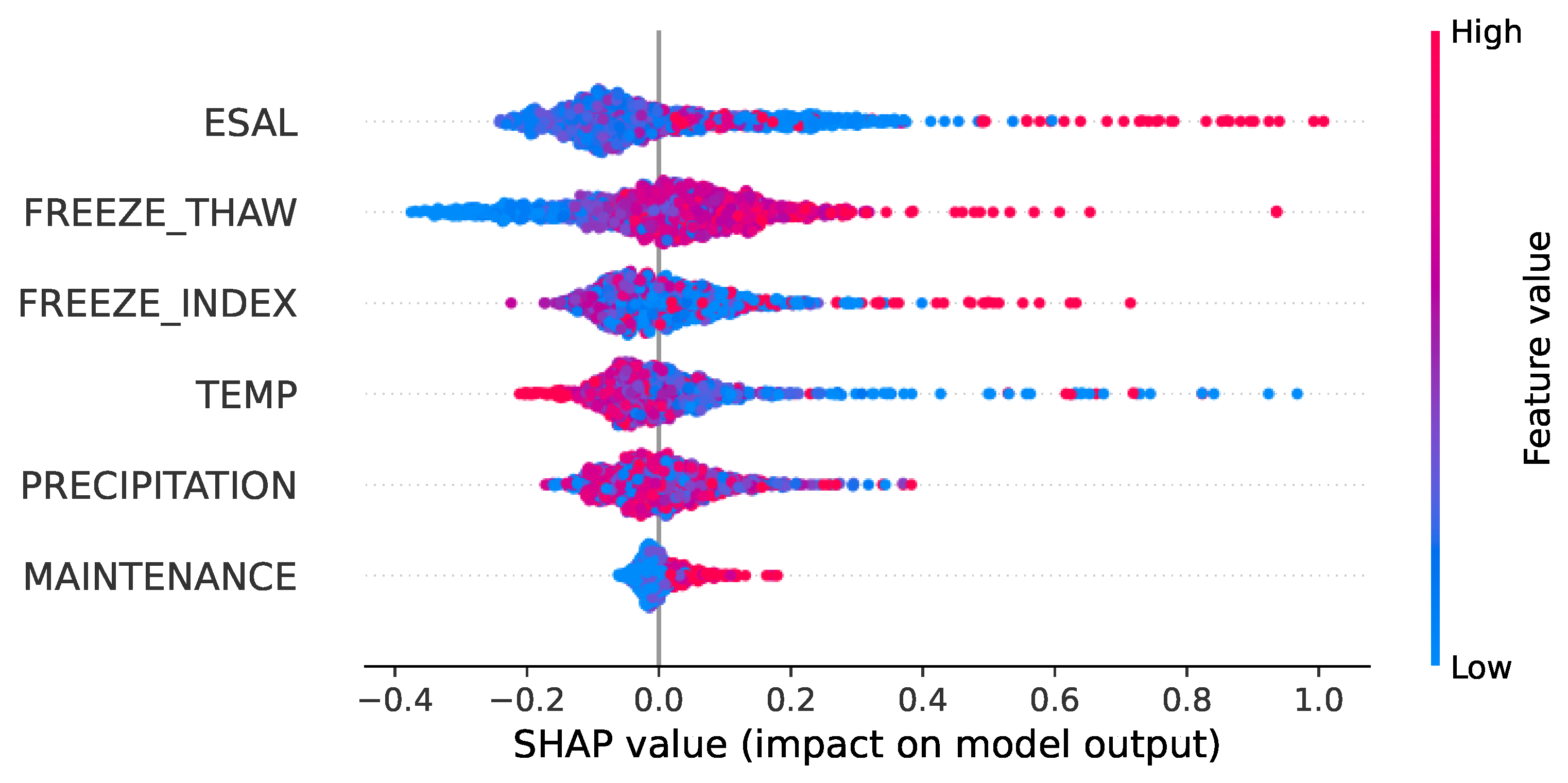
Moreover, based on the SHAP values, it is possible to plot a SHAP feature summary plot, providing a global interpretation of SHAP. Each point in the SHAP feature summary plot represents a real sample, and the color of the point reflects the size of the factor value, the larger value being redder and the smaller value being bluer. The horizontal coordinate is the SHAP value to measure the degree of contribution and impact of the influencing factors on the predicted values of the model, with positive and negative values representing positive or negative contributions, respectively. The vertical coordinate represents the importance of each feature.

3.4.3. Partial Dependence Plots (PDPs)

PDPs show the marginal benefit of one or two features on the predicted outcome of a model. PDPs observe the change in the predicted output of the model when the value of the target feature changes by fixing the values of the other features. There are two forms of PDPs: single-factor PDPs focus on the effect of a single feature on the predicted results, and two-feature interactive PDPs analyze the effect of the interaction between two features on the predicted results of the model. The advantage of PDPs is that they are easy to implement and clear to interpret, but the disadvantage is that PDPs have a limitation in the spatial dimension, which can only respond to two features at most, and at the same time, they need to satisfy the assumption that the features are independent of each other.

4. Results and Discussion

4.1. Feature Selection Results

The results of feature ranking through a voting strategy are shown in Table 7.

Table 7. The results of feature selection.

Feature	Ranking	Feature	Ranking
ESAL	1	AC_THICKNESS	8
TEMP	2	HUMIDITY	9
FREEZE_THAW	3	DRAINAGE_TYPE	10
FREEZE_INDEX	4	MAINTENANCE	11
CLOUD_COVER	5	WIND	12
GB_THICKNESS	6	SUBGRADE_MATL	13
PRECIPITATION	7

Based on the results of feature selection and considering the literature studies on pavement roughness, this paper finally selects ESAL, TEMP, PRECIPITATION, FREEZE_THAW, FREEZE_INDEX and MAINTENANCE as input variables for the pavement roughness prediction model. Although CLOUD_COVER and GB_THICKNESS ranked higher than PRECIPITATION and MAINTENANCE, they were excluded from the model. GB_THICKNESS was excluded because its influence is closely related to the structural capacity already represented by ESAL, reducing the need for additional structural input variables. PRECIPITATION was chosen over CLOUD_COVER because it directly impacts moisture content within the pavement structure, while CLOUD_COVER is an indirect climate-related factor. MAINTENANCE was included despite its lower ranking, since it provides critical insights that are not captured by structural or environmental variables. The selected features aim to balance model interpretability and predictive performance, ensuring the inclusion of variables with the most direct physical relevance of IRI. The effect of feature selection in this study is shown in Table 8.

Table 8. The effectiveness of feature selection.

Name	Time Taken	Memory Used	MSE	${\mathit{R}}^2$
all features	1.0729 s	9.34 MB	0.0801	0.7111
selected features	0.5956 s	9.72 MB	0.0778	0.7194

As can be seen from Table 8, after feature selection, the model brings a significant optimization in time consumption and a small improvement in prediction performance, although the memory saving is not significant. This reflects the effectiveness of the feature selection method in this study.

4.2. Results Comparison and Analysis

4.2.1. Evaluation Metrics

In this study, four evaluation metrics, namely, $MAE$, $MAPE$, $RMSE$ and $R^2$, are adopted to measure the model’s performance. In addition, we evaluate the model’s complexity and the prediction time. The calculation of the four evaluation metrics is defined as follows:

$$MAE={\displaystyle \frac{1}{n}}\sum _{i=1}^n\left|(IR{I}_i-{\widehat{IRI}}_i)\right|$$

(13)

$$MAPE={\displaystyle \frac{100\%}{n}}\sum _{i=1}^n|{\displaystyle \frac{{\widehat{IRI}}_i-IR{I}_i}{IR{I}_i}}|$$

(14)

$$RMSE=\sqrt{{\displaystyle \frac{1}{n}}\sum _{i=1}^n{(IR{I}_i-{\widehat{IRI}}_i)}^2}$$

(15)

$$R^2=1-{\displaystyle \frac{{\sum }_{i=1}^n{(IR{I}_i-{\widehat{IRI}}_i)}^2}{{\sum }_{i=1}^n{(IR{I}_i-{\overline{IRI}}_i)}^2}}$$

(16)

where detailed variable definitions are provided in Table A3 in Appendix A.

4.2.2. Optimized Hyperparameter Settings

In this study, 5-fold cross-validation ($K=5$) is combined with the grid search method to optimize the hyperparameters. In 5-fold cross-validation, 20% of the training dataset is used as a validation dataset in each iteration, while the remaining 80% of the training dataset is used to train the model. The final results of hyperparameter tuning are shown in Table 9.

Table 9. Parameters of hyperparametric optimization.

Model	Parameter	Grid Search Scope	Determine the Numerical Value
XGBoost	max_depth	[3, 4, 5, 6, 7, 8, 10, 12]	8
	n_estimators	[50, 100, 150, 200, 220, 250, 300, 350, 400, 450, 490, 500, 510]	300
	learning_rate	[0.001, 0.01, 0.05, 0.1, 0.2]	0.05
	gamma	[0.0, 0.1, 0.2]	0.0
	reg_alpha	[0.001, 0.01, 0.1]	0.001
	reg_lambda	[0.01, 0.1, 1]	0.01
	min_child_weight	[2, 3, 4, 5, 6]	3
	colsample_bytree	[0.6, 0.7, 0.8, 0.9]	0.6
	subsample	[0.6, 0.7, 0.8, 0.9]	0.7
Random Forest	n_estimators	[50, 100, 150, 200, 220, 250, 300, 350, 400, 450, 490, 500, 510]	220
	max_depth	[3, 4, 5, 6, 7, 8, 10, 12]	5
	min_samples_split	[2, 5, 8, 10]	2
	min_samples_leaf	[1, 2, 3, 4, 5]	1
	max_features	[‘Sqrt’, ‘Log2’]	Sqrt
	bootstrap	[True, False]	False
GBDT	n_estimators	[50, 100, 150, 200, 220, 250, 300, 350, 400, 450, 490, 500, 510]	500
	learning_rate	[0.01, 0.05, 0.1, 0.15, 0.2]	0.05
	max_depth	[3, 4, 5, 6, 7, 8, 10, 12]	7
	min_samples_split	[2, 5, 10, 15]	10
	min_samples_leaf	[1, 2, 4, 5]	2
	subsample	[0.6, 0.7, 0.8, 0.9, 1.0]	1.0
	max_features	[‘Sqrt’, ‘Log2’, None]	Sqrt

4.2.3. Results of ML Models

Table 10 presents the performance indices for both the training and testing datasets. These indices include critical evaluation metrics such as $MAE$, $MAPE$, $RMSE$ and $R^2$. As can be seen from Table 10, the XGBoost model demonstrated superior training performance, exhibiting a superior fit in comparison to the GBDT and RF models. The XGBoost model demonstrated optimal performance in the testing dataset, as evidenced by its highest $R^2$ value of 0.776 and lowest $RMSE$ of 0.243. This suggests that the model exhibited minimal deviation from the actual values. And the XGBoost model demonstrates a marginal decline in error when comparing the training and test datasets, suggesting that it is not experiencing a significant overfitting issue. In addition, the training and prediction times of ML models are shown in Table A4 in Appendix A. The XGBoost model has a distinct advantage in prediction speed, which is crucial for applications where real time is needed.

Table 10. Performance indices for training and testing data.

ML Models	Training				Test
	MAE	MAPE	RMSE	${\mathit{R}}^{\mathbf{2}}$	MAE	MAPE	RMSE	${\mathit{R}}^{\mathbf{2}}$
RF	0.085	0.074	0.122	0.932	0.194	0.163	0.264	0.736
GBDT	0.020	0.018	0.029	0.956	0.187	0.160	0.254	0.756
XGBoost	0.030	0.033	0.042	0.987	0.186	0.159	0.243	0.778

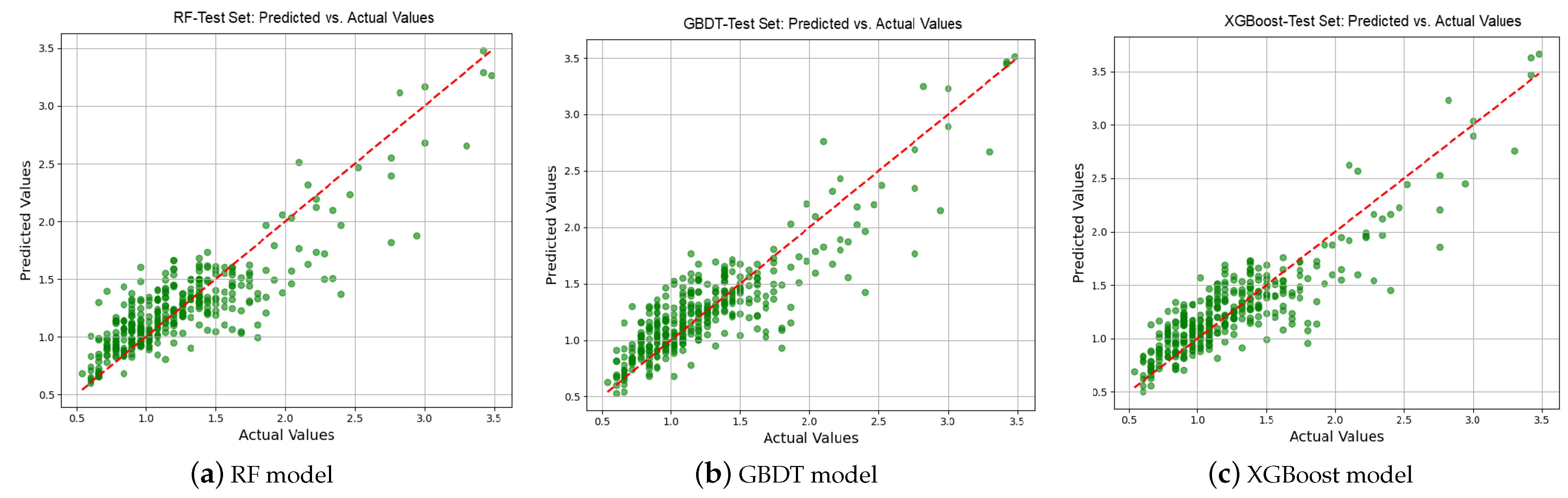
Figure 7 shows the scatter plots, which present the relationship between the predicted and actual values for the test dataset. The scatter plot for XGBoost shows a strong linear trend with most points clustering closely around the red dashed line, indicating superior accuracy. The XGBoost model outperforms both the RF and GBDT models in terms of prediction accuracy and generalization. Thus, this study performs key influencing factors’ interpretable analysis on the basis of an XGBoost-based prediction model.

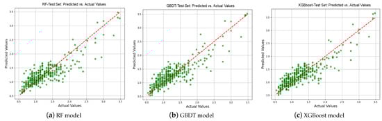
Figure 7. Predicted versus observed IRI: RF, GBDT and XGBoost.

4.3. Feature Importance Analysis

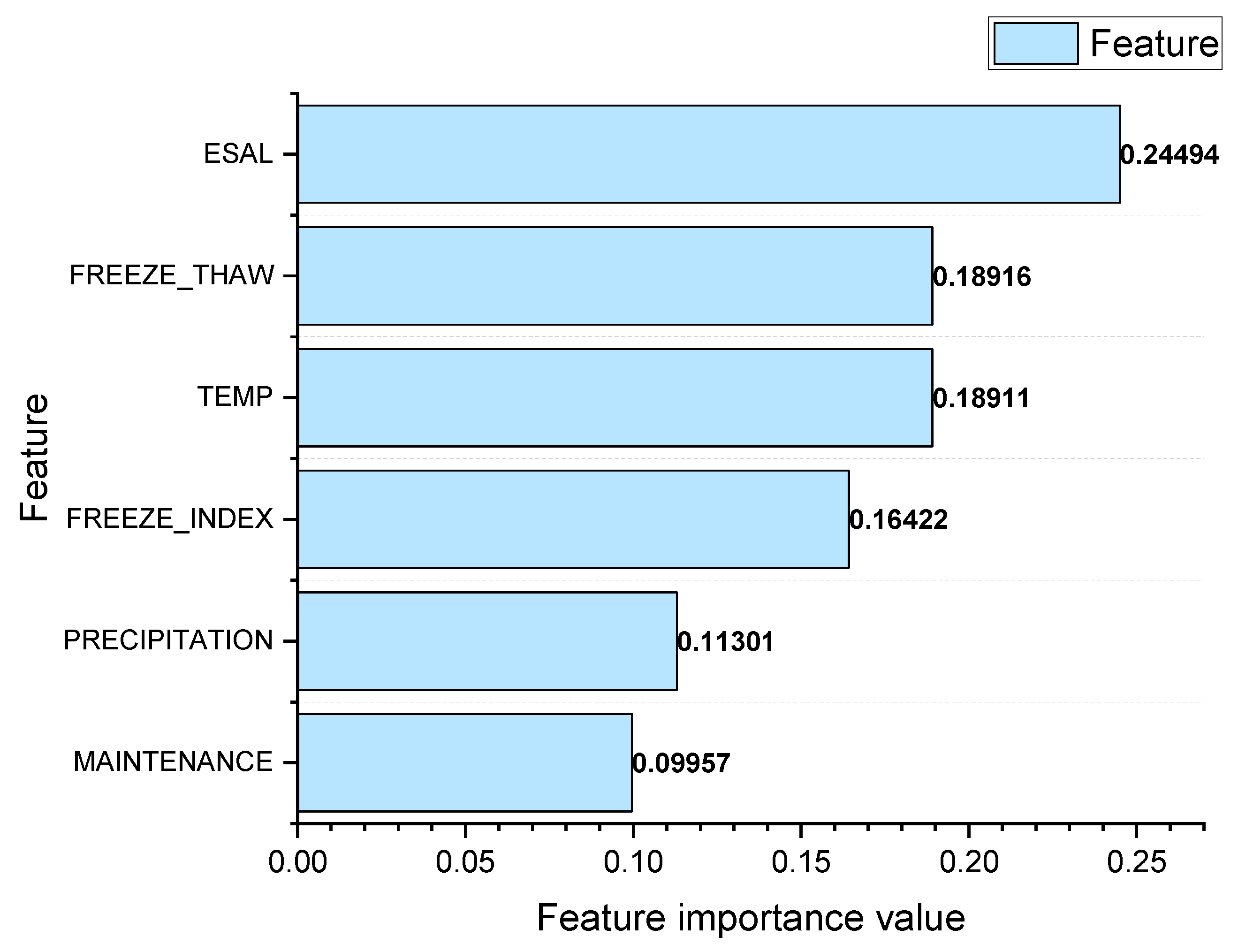
Through the proposed IRI prediction model based on XGBoost, the ranking of key factors is shown in Figure 8.

Figure 8. Feature importance.

As can be seen in Figure 8, there are differences in the importance of each independent variable to pavement roughness. The feature importance values of the equivalent number of actions of a standard axle load, number of freeze–thaw cycles, annual average temperature, freezing index, annual precipitation and road section maintenance times were 0.24494, 0.18916, 0.18911, 0.16422, 0.11301 and 0.09957, respectively. The results showed that the equivalent number of actions of a standard axle load, number of freeze–thaw cycles and annual average temperature have a significant effect on pavement roughness. The freezing index and annual average temperature are next in importance, and road section maintenance times have the least impact. And the differences in Table 7 and Figure 8 are expected due to the contrasting purposes of the two analysis methods. Feature selection aims to reduce dimensionality and identify the key influencing factors, whereas feature importance in the XGBoost model reflects both direct contributions and interactions within the fitted model structure.

4.4. Factor Analysis Based on SHAP

The SHAP summary plot in this study is shown in Figure 9.

Figure 9. SHAP summary plot.

As depicted in Figure 9, for the equivalent number of actions of a standard axle load, number of freeze–thaw cycles and freezing index, the vast majority of the red points are located on the right side, indicating that larger values of these features have positive effects on IRI prediction. It shows that higher traffic load, frequent freeze–thaw cycles and higher freezing index deteriorate pavement roughness. For annual average temperature, the positive effects predicted by the model can come from both higher and lower temperature, indicating that extreme temperature conditions can degrade pavement roughness. For the annual average temperature, the model predicts positive effects on IRI from both higher and lower temperature. This indicates that extreme temperature conditions can exacerbate pavement roughness. In practical terms, this suggests that regions with significant temperature fluctuations or extreme climate conditions are more likely to experience rapid pavement deterioration.

These findings are consistent with existing research and have practical implications for road maintenance strategies. Heavy traffic loading could exert a greater force on the road and then damage the pavement surface characteristics of an even pavement structure, thus increasing the IRI value [21]. The average temperature/freezing index of the weak precipitation area is low/high, and cold cracking is prone to occur due to cycles of freezing and thawing, leading to a deterioration in the performance of pavement surface roughness [55].

4.5. Factor Analysis Based on PDPs

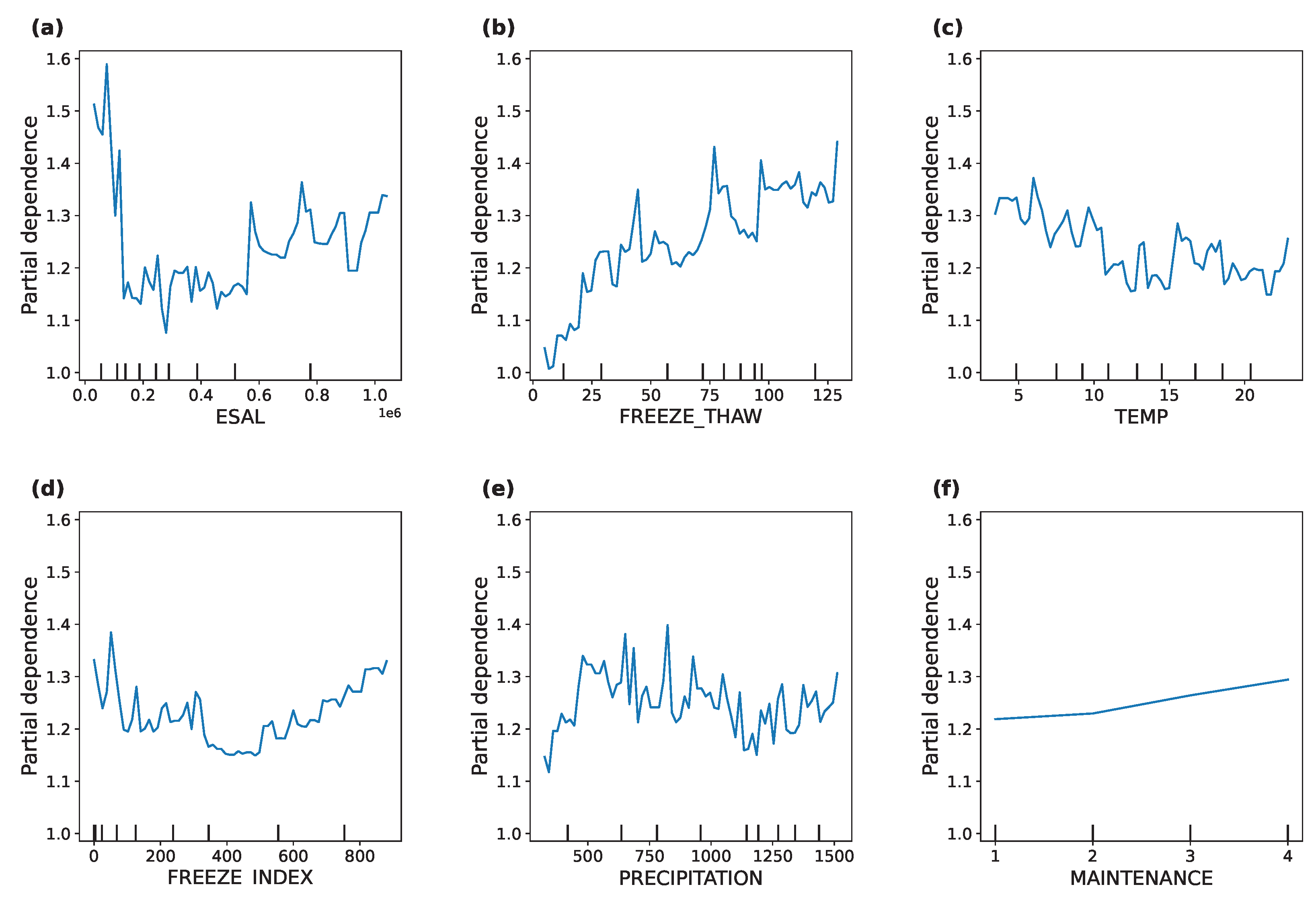
In this study, the single-factor PDPs of the equivalent number of actions of a standard axle load, annual average temperature, number of freeze–thaw cycles, freezing index, annual precipitation and road section maintenance times were analyzed, and the results obtained are shown in Figure 10.

Figure 10. Partial dependence plots. (a) ESAL. (b) FREEZE_THAW. (c) TEMP. (d) FREEZE INDEX. (e) PRECIPITATION. (f) MAINTENANCE.

(1)

The effect of the equivalent number of actions of a standard axle load on pavement roughness, as shown in Figure 10a. As the equivalent number of actions of a standard axle load approaches 0, IRI is high, but as the equivalent number of actions of a standard axle load increases, the IRI value decreases and stabilizes. And ultimately, as the equivalent number of actions of a standard axle load rises, IRI again shows an increasing trend. This is because as the traffic load increases, the pavement improves initially due to compaction. But excessive traffic loads can exacerbate the damage to the pavement structure and lead to deterioration in pavement roughness.

(2)

The effect of the number of freeze–thaw cycles on pavement roughness, as illustrated in Figure 10b. As the number of freeze–thaw cycles increases, the IRI value gradually increases. It indicates that the freeze–thaw cycles have a significant negative effect on pavement roughness. During the freeze–thaw cycle, the pavement material undergoes repeated expansion and contraction due to temperature changes, which ultimately leads to cracking and damage to the pavement, thus affecting the roughness.

(3)

The effect of annual average temperature on pavement roughness, as depicted in Figure 10c. With the increase in temperature, IRI showed a gradual decrease, and IRI was higher under low-temperature conditions. As the temperature increased, the IRI gradually decreased, and after the temperature increased to a certain extent, IRI increased. This shows that pavement materials become brittle at low temperatures and are prone to cracking and breaking, resulting in uneven pavements. As the temperature rises, the material becomes more flexible in warmer climates and is able to maintain better roughness. In high-temperature environments, pavement deterioration problems can occur, resulting in uneven pavement surfaces.

(4)

The effect of freezing index on pavement roughness, as presented in Figure 10d. The influence curve of the freezing index on the IRI shows some fluctuation. When the freezing index is low, the IRI value has a slight tendency to decrease, while as the freezing index increases, the IRI value gradually increases. This shows that a higher freezing index can exacerbate pavement damage caused by freeze–thaw cycles, leading to a reduction in pavement roughness.

(5)

The effect of annual precipitation on pavement roughness, as described in Figure 10e. The increase in precipitation has resulted in a fluctuating upward trend in IRI values. This is because the moisture penetrates into the pavement structure, leading to a softening of the road base and a reduction in the strength of the pavement. It will exacerbate the unevenness of the pavement.

(6)

The effect of road section maintenance times on pavement roughness, as demonstrated in Figure 10f. The frequency of pavement maintenance is found to be positively correlated with IRI values, with higher levels of maintenance resulting in higher IRI values. This may be due to the observation that more frequently maintained road sections tend to have higher levels of damage. It can be hypothesized that road sections that are subject to higher levels of maintenance may have higher IRI values and therefore require more frequent maintenance.

5. Conclusions

Road maintenance and management are complex due to limited resources and extensive pavement networks. Predicting pavement performance using data-driven methods offers a comprehensive approach to improving maintenance strategies. The objective of this study is to achieve an accurate prediction of IRI using advanced ML techniques, providing scientific support for maintenance.

This study introduced an explainable boosting method based on XGBoost, which effectively identifies key influencing factors and predicts IRI. We constructed a high-quality, multi-dimensional pavement roughness dataset using the LTPP database. After the voting-based feature selection, the key factors influencing IRI were identified. Through the comparison of ML models, the proposed XGBoost-based IRI prediction model achieved an $R^2$ value of 0.778. Using explainable methods such as feature importance, SHAP and PDPs, this study revealed the specific mechanism of each influencing factor on IRI. The following conclusions can be drawn:

(1)

Key factor identification. The integrated feature selection method results identified six key factors that affect the pavement roughness the most: ESAL, FREEZE_THAW, FREEZE_INDEX, TEMP, PRECIPITATION and MAINTENANCE.

(2)

Significance of key factors analysis. For IRI analysis, ESAL has a significant influence on the pavement roughness. And climate factors should be considered as part of pavement roughness. Although PRECIPITATION and MAINTENANCE exhibit relatively low direct contributions in the model, their roles in maintaining pavement roughness and extending the service life of the road should not be ignored.

(3)

Interpretable analysis. Through the SHAP and PDP analysis based on XGBoost, we can conclude that high traffic loads, frequent freeze–thaw cycles and large freezing indices significantly contribute to pavement unevenness. Under extreme temperature conditions, both high and low temperatures can exacerbate pavement roughness, emphasizing the importance of accounting for temperature change in pavement management strategies.

Practically, the identification of key influencing factors and the explainable analysis provide data-driven support for the pavement management department to develop maintenance strategies. The developed XGBoost-based IRI prediction model can guide professionals to make more informed decisions about road maintenance. For example, in areas with extreme climatic conditions, such as low- and high-temperature areas, pavement materials with excellent resistance to cracking and thermal aging, respectively, should be used to reduce the adverse effects of extreme temperatures on pavements. In areas with frequent freeze–thaw cycles and high freeze index, it is necessary to strengthen the design of the waterproof layer of the road surface and ensure the normal operation of the drainage system.

Although this study has considered pavement structure, climate and traffic factors, it does not account for temporal continuity in the IRI prediction model. Future research should use historical IRI values to construct a more time-sensitive prediction model. At the same time, customizing a fine-grained dataset with labels reflecting geographic or climatic conditions and thus enabling the model to provide tailored recommendations for construction and maintenance strategies is worth further in-depth study. In order to present a broader perspective on feature impact and interaction, integrating newer explainability techniques (e.g., LIME [56]) alongside SHAP would be part of the future extension of the research.

References

- Wang, H.; Huo, N.; Li, J.; Wang, K.; Wang, Z. A road quality detection method based on the mahalanobis-taguchi system. IEEE Access 2018, 6, 29078–29087. [Google Scholar] [CrossRef]
- Kaloop, M.R.; El-Badawy, S.M.; Ahn, J.; Sim, H.B.; Hu, J.W.; Abd El-Hakim, R.T. A hybrid wavelet-optimally-pruned extreme learning machine model for the estimation of international roughness index of rigid pavements. Int. J. Pavement Eng. 2022, 23, 862–876. [Google Scholar] [CrossRef]
- Wu, D. Ride Comfort Prediction on Urban Road Using Discrete Pavement Roughness Index. Appl. Sci. 2024, 14, 3108. [Google Scholar] [CrossRef]
- Al-Mansour, A.I.; Shokri, A.A. Correlation of pavement distress and roughness measurement. Appl. Sci. 2022, 12, 3748. [Google Scholar] [CrossRef]
- Dalla Rosa, F.; Liu, L.; Gharaibeh, N.G. IRI prediction model for use in network-level pavement management systems. J. Transp. Eng. Part B Pavements 2017, 143, 04017001. [Google Scholar] [CrossRef]
- Abdelaziz, N.; Abd El-Hakim, R.T.; El-Badawy, S.M.; Afify, H.A. International Roughness Index prediction model for flexible pavements. Int. J. Pavement Eng. 2020, 21, 88–99. [Google Scholar] [CrossRef]
- Lina, Z.; Dongpo, H.; Qianqian, Z. Modeling of international roughness index in seasonal frozen area. Mag. Civ. Eng. 2021, 104, 10402. [Google Scholar]
- Bueno, L.D.; Pereira, D.d.S.; Specht, L.P.; Nascimento, L.A.H.d.; Schuster, S.L.; Fritzen, M.A.; Kim, Y.R.; Back, A.H. Contribution to the mechanistic-empirical roughness prediction in asphalt pavements. Road Mater. Pavement Des. 2023, 24, 690–705. [Google Scholar] [CrossRef]
- Moreira, A.V.; Tinoco, J.; Oliveira, J.R.; Santos, A. An application of Markov chains to predict the evolution of performance indicators based on pavement historical data. Int. J. Pavement Eng. 2018, 19, 937–948. [Google Scholar] [CrossRef]
- Pérez-Acebo, H.; Mindra, N.; Railean, A.; Rojí, E. Rigid pavement performance models by means of Markov Chains with half-year step time. Int. J. Pavement Eng. 2019, 20, 830–843. [Google Scholar] [CrossRef]
- El-Khawaga, M.; El-Badawy, S.; Gabr, A. Comparison of master sigmoidal curve and Markov chain techniques for pavement performance prediction. Arab. J. Sci. Eng. 2020, 45, 3973–3982. [Google Scholar] [CrossRef]
- Jiang, Y.; Li, S. Gray system model for estimating the pavement international roughness index. J. Perform. Constr. Facil. 2005, 19, 62–68. [Google Scholar] [CrossRef]
- Yu, J.; Zhang, X.; Xiong, C. A methodology for evaluating micro-surfacing treatment on asphalt pavement based on grey system models and grey rational degree theory. Constr. Build. Mater. 2017, 150, 214–226. [Google Scholar] [CrossRef]
- Zhang, X.; Ji, C. Asphalt pavement roughness prediction based on gray GM (1, 1| sin) model. Int. J. Comput. Intell. Syst. 2019, 12, 897–902. [Google Scholar] [CrossRef]
- Wang, X.; Zhao, J.; Li, Q.; Fang, N.; Wang, P.; Ding, L.; Li, S. A hybrid model for prediction in asphalt pavement performance based on support vector machine and grey relation analysis. J. Adv. Transp. 2020, 2020, 7534970. [Google Scholar] [CrossRef]
- Sharma, A.; Aggarwal, P. IRI Prediction using Machine Learning Models. WSEAS Trans. Comput. Res. 2023, 11, 111–116. [Google Scholar] [CrossRef]
- Qiao, Y.; Chen, S.; Alinizzi, M.; Alamaniotis, M.; Labi, S. IRI estimation based on pavement distress type, density, and severity: Efficacy of machine learning and statistical techniques. J. Infrastruct. Syst. 2022, 28, 04022035. [Google Scholar] [CrossRef]
- Gong, H.; Sun, Y.; Shu, X.; Huang, B. Use of random forests regression for predicting IRI of asphalt pavements. Constr. Build. Mater. 2018, 189, 890–897. [Google Scholar] [CrossRef]
- Marcelino, P.; de Lurdes Antunes, M.; Fortunato, E.; Gomes, M.C. Machine learning approach for pavement performance prediction. Int. J. Pavement Eng. 2021, 22, 341–354. [Google Scholar] [CrossRef]
- Guo, X.; Hao, P. Using a random forest model to predict the location of potential damage on asphalt pavement. Appl. Sci. 2021, 11, 10396. [Google Scholar] [CrossRef]
- Luo, Z.; Zhan, Y.; Liu, Y.; Zhang, A.; Lin, X.; Zhang, Y. Research on influencing factors of asphalt pavement international roughness index (IRI) based on ensemble learning. Intell. Transp. Infrastruct. 2022, 1, liac014. [Google Scholar] [CrossRef]
- Damirchilo, F.; Hosseini, A.; Mellat Parast, M.; Fini, E.H. Machine learning approach to predict international roughness index using long-term pavement performance data. J. Transp. Eng. Part B Pavements 2021, 147, 04021058. [Google Scholar] [CrossRef]
- El-Hakim, R.T.A.; Awaad, A.N.; El-Badawy, S.M. Machine Learning-Based Prediction of International Roughness Index for Continuous Reinforced Concrete Pavements. Mansoura Eng. J. 2024, 49, 14. [Google Scholar] [CrossRef]
- Wang, C.; Xu, S.; Yang, J. Adaboost algorithm in artificial intelligence for optimizing the IRI prediction accuracy of asphalt concrete pavement. Sensors 2021, 21, 5682. [Google Scholar] [CrossRef] [PubMed]
- Teomete, E.; Bayrak, M.B.; Agarwal, M. Use of artificial neural networks for predicting rigid pavement roughness. In Proceedings of the 2004 Transportation Scholars ConferenceIowa State University, Ames, IA, USA, 19 November 2004. [Google Scholar]
- Sollazzo, G.; Fwa, T.; Bosurgi, G. An ANN model to correlate roughness and structural performance in asphalt pavements. Constr. Build. Mater. 2017, 134, 684–693. [Google Scholar] [CrossRef]
- Zeiada, W.; Dabous, S.A.; Hamad, K.; Al-Ruzouq, R.; Khalil, M.A. Machine learning for pavement performance modelling in warm climate regions. Arab. J. Sci. Eng. 2020, 45, 4091–4109. [Google Scholar] [CrossRef]
- Hossain, M.; Gopisetti, L.; Miah, M. International roughness index prediction of flexible pavements using neural networks. J. Transp. Eng. Part B Pavements 2019, 145, 04018058. [Google Scholar] [CrossRef]
- Nguyen, H.L.; Pham, B.T.; Son, L.H.; Thang, N.T.; Ly, H.B.; Le, T.T.; Ho, L.S.; Le, T.H.; Tien Bui, D. Adaptive network based fuzzy inference system with meta-heuristic optimizations for international roughness index prediction. Appl. Sci. 2019, 9, 4715. [Google Scholar] [CrossRef]
- Ziari, H.; Sobhani, J.; Ayoubinejad, J.; Hartmann, T. Prediction of IRI in short and long terms for flexible pavements: ANN and GMDH methods. Int. J. Pavement Eng. 2016, 17, 776–788. [Google Scholar] [CrossRef]
- Múčka, P. International Roughness Index specifications around the world. Road Mater. Pavement Des. 2017, 18, 929–965. [Google Scholar] [CrossRef]
- Xin, L.; Zhenzhen, X.; Lili, P.; Jun, H.; Yaohui, D. A new model for predicting IRI using TabNet with hunter-prey optimization. Int. J. Pavement Eng. 2024, 25, 2414070. [Google Scholar] [CrossRef]
- Federal Highway Administration. LTPP InfoPave: Long-Term Pavement Performance Data Analysis. 2024. Available online: https://infopave.fhwa.dot.gov/Data/DataSelection (accessed on 18 November 2024).
- Gong, H.; Sun, Y.; Hu, W.; Polaczyk, P.A.; Huang, B. Investigating impacts of asphalt mixture properties on pavement performance using LTPP data through random forests. Constr. Build. Mater. 2019, 204, 203–212. [Google Scholar] [CrossRef]
- Li, M.; Dai, Q.; Su, P.; You, Z.; Ma, Y. Surface layer modulus prediction of asphalt pavement based on LTPP database and machine learning for Mechanical-Empirical rehabilitation design applications. Constr. Build. Mater. 2022, 344, 128303. [Google Scholar] [CrossRef]
- Zhang, M.; Gong, H.; Jia, X.; Xiao, R.; Jiang, X.; Ma, Y.; Huang, B. Analysis of critical factors to asphalt overlay performance using gradient boosted models. Constr. Build. Mater. 2020, 262, 120083. [Google Scholar] [CrossRef]
- Wang, C.; Xiao, W.; Liu, J. Developing an improved extreme gradient boosting model for predicting the international roughness index of rigid pavement. Constr. Build. Mater. 2023, 408, 133523. [Google Scholar] [CrossRef]
- García, S.; Luengo, J.; Herrera, F. Data Preprocessing in Data Mining; Springer: Cham, Switzerland, 2015; Volume 72. [Google Scholar]
- Ni, L.; Wang, Y.; Wang, J.; Dong, W.; Liu, H.; Xing, Y.; Darong, H.; Lanyan, K. A synergetic locating method for abnormal interval of stacker safety maintenance. Syst. Sci. Control Eng. 2018, 6, 169–176. [Google Scholar] [CrossRef]
- Mustaqim, A.Z.; Adi, S.; Pristyanto, Y.; Astuti, Y. The effect of recursive feature elimination with cross-validation (RFECV) feature selection algorithm toward classifier performance on credit card fraud detection. In Proceedings of the 2021 International Conference on Artificial Intelligence and Computer Science Technology (ICAICST), Yogyakarta, Indonesia, 29–30 June 2021; IEEE: Piscataway, NJ, USA, 2021; pp. 270–275. [Google Scholar]
- Awad, M.; Fraihat, S. Recursive feature elimination with cross-validation with decision tree: Feature selection method for machine learning-based intrusion detection systems. J. Sens. Actuator Netw. 2023, 12, 67. [Google Scholar] [CrossRef]
- Vergara, J.R.; Estévez, P.A. A review of feature selection methods based on mutual information. Neural Comput. Appl. 2014, 24, 175–186. [Google Scholar] [CrossRef]
- Elavarasan, D.; Vincent PM, D.R.; Srinivasan, K.; Chang, C.Y. A hybrid CFS filter and RF-RFE wrapper-based feature extraction for enhanced agricultural crop yield prediction modeling. Agriculture 2020, 10, 400. [Google Scholar] [CrossRef]
- Muthukrishnan, R.; Rohini, R. LASSO: A feature selection technique in predictive modeling for machine learning. In Proceedings of the 2016 IEEE International Conference on Advances in Computer Applications (ICACA), Coimbatore, India, 24 October 2016; IEEE: Piscataway, NJ, USA, 2016; pp. 18–20. [Google Scholar]
- Breiman, L. Random forests. Mach. Learn. 2001, 45, 5–32. [Google Scholar] [CrossRef]
- Zhang, C.; Zhang, Y.; Shi, X.; Almpanidis, G.; Fan, G.; Shen, X. On incremental learning for gradient boosting decision trees. Neural Process. Lett. 2019, 50, 957–987. [Google Scholar] [CrossRef]
- Rao, H.; Shi, X.; Rodrigue, A.K.; Feng, J.; Xia, Y.; Elhoseny, M.; Yuan, X.; Gu, L. Feature selection based on artificial bee colony and gradient boosting decision tree. Appl. Soft Comput. 2019, 74, 634–642. [Google Scholar] [CrossRef]
- Cheng, J.; Li, G.; Chen, X. Research on travel time prediction model of freeway based on gradient boosting decision tree. IEEE Access 2018, 7, 7466–7480. [Google Scholar] [CrossRef]
- Chen, T.; Guestrin, C. XGBoost: A scalable tree boosting system. In Proceedings of the 22nd ACM SIGKDD International Conference on Knowledge Discovery and Data Mining, San Francisco, CA, USA, 13–17 August 2016; pp. 785–794. [Google Scholar]
- Wakjira, T.G.; Ibrahim, M.; Ebead, U.; Alam, M.S. Explainable machine learning model and reliability analysis for flexural capacity prediction of RC beams strengthened in flexure with FRCM. Eng. Struct. 2022, 255, 113903. [Google Scholar] [CrossRef]
- Kazemi, F.; Asgarkhani, N.; Jankowski, R. Optimization-based stacked machine-learning method for seismic probability and risk assessment of reinforced concrete shear walls. Expert Syst. Appl. 2024, 255, 124897. [Google Scholar] [CrossRef]
- Li, Z. Extracting spatial effects from machine learning model using local interpretation method: An example of SHAP and XGBoost. Comput. Environ. Urban Syst. 2022, 96, 101845. [Google Scholar] [CrossRef]
- Lundberg, S. A unified approach to interpreting model predictions. arXiv 2017, arXiv:1705.07874. [Google Scholar]
- Cakiroglu, C.; Demir, S.; Ozdemir, M.H.; Aylak, B.L.; Sariisik, G.; Abualigah, L. Data-driven interpretable ensemble learning methods for the prediction of wind turbine power incorporating SHAP analysis. Expert Syst. Appl. 2024, 237, 121464. [Google Scholar] [CrossRef]
- Zhao, X.; Shen, A.; Ma, B. Temperature response of asphalt pavement to low temperatures and large temperature differences. Int. J. Pavement Eng. 2020, 21, 49–62. [Google Scholar] [CrossRef]
- Ribeiro, M.T.; Singh, S.; Guestrin, C. “Why should i trust you?” Explaining the predictions of any classifier. In Proceedings of the ACM SIGKDD International Conference on Knowledge Discovery and Data Mining, San Francisco, CA, USA, 13–17 August 2016; pp. 1135–1144. [Google Scholar]
Disclaimer/Publisher’s Note: The statements, opinions and data contained in all publications are solely those of the individual author(s) and contributor(s) and not of MDPI and/or the editor(s). MDPI and/or the editor(s) disclaim responsibility for any injury to people or property resulting from any ideas, methods, instructions or products referred to in the content. |
© 2025 by the authors. Licensee MDPI, Basel, Switzerland. This article is an open access article distributed under the terms and conditions of the Creative Commons Attribution (CC BY) license (https://creativecommons.org/licenses/by/4.0/).