Validation of Computational Methods for Free-Water Jet Diffusion and Pressure Dynamics in a Plunge Pool

Abstract

This study investigates the numerical modeling of a high-velocity circular free-water jet impinging into a plunge pool, focusing on the simulation and validation of mean and fluctuating dynamic pressures on the pool floor. Numerical simulations were performed using two different computation methods, two-phase volume-of-fluid and Euler–Euler, under conditions replicating experimental data obtained at a jet velocity of 7.4 m/s and plunge pool depth of 0.8 m. The models, based respectively on the Volume of Fluid (VoF) and Euler–Euler methods, were evaluated for accuracy in replicating experimentally measured pressures and air concentration values. The Euler–Euler solver, coupled with the k-Omega SST turbulence model, demonstrated mesh independence for mean dynamic pressures with a mesh resolution of 24 cells across the jet diameter. In contrast, two-phase volume-of-fluid exhibited mesh dependency, particularly near the jet stagnation point and pressure values higher than the experimental ones. While the Euler–Euler accurately captured mean pressures and air concentration in close agreement with experimental data, its Reynolds-Averaged Navier–Stokes (RANS) formulation limited its ability to simulate pressure fluctuations directly. To approximate these fluctuations, turbulent kinetic energy values were used to derive empirical estimates, yielding results consistent with experimental measurements. This study demonstrates the efficacy of the Euler–Euler method with the k-Omega SST model in accurately capturing key dynamic pressures and air entrainment in plunge pools while highlighting opportunities for future work on pressure fluctuation modeling across a broader range of jet conditions.

1. Introduction

1.1. Background of High-Velocity Free-Water Jets

Dam safety standards require effective floodwater management, often achieved through the use of spillways, which convey water at high velocities during flood events.

The use of high-velocity free-water jets for floodwater conveyance is a cost-effective alternative to long chutes or tunnels. Spillways are designed with hydraulic structures to effectively handle these turbulent water jets during flood events. These high-velocity turbulent flows impinge on and diffuse within plunge pools downstream, where they are deflected by the solid surfaces or the riverbed, such as rock or concrete. The high-velocity jet plunge pool diffusion and wall jet development after deflection facilitate efficient energy dissipation but also present significant challenges for modeling and predicting flow velocities, turbulent pressures, and overall stream power [1,2].

These high-velocity free-water jets present unique challenges regarding hydraulic performance and energy dissipation in downstream plunge pools. In fact, during flood discharges, water flows with much higher velocities and pressures than before dam construction, significantly altering the hydraulic conditions. To achieve the final design for the spillways, theoretical formulations were used alongside a physical model. Advanced computational modeling of flow is also applied to predict flow behavior accurately.

1.2. Previous Research on High-Velocity Jet Behavior

Characterizing the flow of a jet at the impinging section and the interaction with the bottom of the plunge pool is crucial, and previous studies have focused on the mean and fluctuating pressures, often treating them as non-dimensional parameters relative to the impinging jet velocity [3,4,5,6,7,8]. However, this approach overlooks scale effects related to jet velocity, plunge pool size, and aeration, which are critical for an accurate simulation and proper design [9]. Bollaert [10] conducted experiments using a jet with a diameter of 0.072 m, studying the pressure field at the plunge pool bottom and within a rock joint for jets with velocities up to 37.2 m/s. This work provides valuable insights into the pressure distribution relevant to understanding the behavior of high-velocity jets in plunge pools. Manso [11] explored the influence of plunge pool geometry on rock scour, while Duarte [12] assessed the stability of rock blocks subjected to high-velocity free-water jets, with velocities ranging from 4.9 to 22.1 m/s and air concentrations from 0% to 23%. Federspiel [13] continued this line of research, examining the response of rock blocks in terms of pressures and accelerations. Jamet et al. [14] experimentally characterized dynamic pressures near the stagnation zone for circular jets. These studies highlight the importance of understanding the interaction between jet velocity, air-water mixtures, and solid boundaries in high-velocity jet applications.

1.3. Numerical Approaches to Modeling High-Velocity Jets

Numerical simulations of free-water jets in the atmosphere [15] and within plunge pools have provided insights into jet behavior, including pressure fields at the stagnation point. However, challenges remain in accurately modeling the complex interactions, particularly in high-velocity, turbulent flows, and air-water interactions [16,17,18]. These include accurately modeling the turbulence and shear forces in the flow, assessing the turbulent flow components, and capturing air-water interactions. The complexity of accurately simulating plunge pool flows is exacerbated by mesh sensitivity and near-wall boundary layer dynamics, mainly using methods like two-phase volume-of-fluid and Euler–Euler. Addressing these challenges requires a careful selection of flow simulation and turbulence models, as well as discretization schemes, along with rigorous validation against reliable experimental data.

Castillo et al. [19] analyzed the velocity profile and pressures at the stagnation point of free rectangular jets, providing valuable data for understanding jet behavior in plunge pools. Their numerical simulations agreed with experimental data regarding the velocity profile and pressure estimates near the stagnation point. Anirban et al. [20] conducted a numerical simulation of a free water jet in the atmosphere, which yielded reasonable agreement with experimental data for velocity, pressure, and volume fraction. Castillo et al. [21] further analyzed mean velocity and turbulent kinetic energy within a plunge pool, achieving good correspondence between experimental data and theoretical models. Badas et al. [22] simulated a physical model of a spillway using the Volume of Fluid (VoF) method, concluding that it adequately simulated important variables such as water depths in the plunge pool and pressures at the jet impact area. Maleki et al. [23] conducted numerical simulations of a jet impacting a plunge pool, comparing their findings with experimental data obtained using k-Epsilon and Detached Eddy Simulation (DES) models for turbulence. They considered a jet velocity of 6.0 m/s, and good agreement was found for pressure readings at the plunge pool bottom. These authors successfully replicated pressure fluctuations that aligned with experimental results using the DES model, although their simulations were limited to a single-phase (water) flow, excluding air-water interactions. Notably, both experimental and CFD pressure fluctuation data were acquired at a frequency of 100 Hz, which, given the presence of significant energy content at higher frequencies, may introduce uncertainty in the measured pressure fluctuations [10,11,12,13,14,24].

Xiangju and Xuewei [16] compared the various two-phase volume-of-fluid and Euler–Eulers, concluding that the Euler–Euler approach is more suitable for modeling two-phase water-air flows. Similarly, Mendes et al. [18] evaluated the efficiency of twoPhaseEulerFoam relative to the InterFoam-VoF solver in modeling a spillway aerator. They found that the Euler–Euler solver provided better cost-efficiency and significant advantages for hydraulic engineering applications involving aerated spillway flows.

1.4. Objective of the Study

This study evaluates the capability of two numerical methods, two-phase volume-of-fluid and Euler–Euler, in replicating the behavior of a high-velocity free-water jet impacting a plunge pool. Specifically, it aims to assess their performance in predicting mean dynamic pressures and air concentration, as well as their accuracy in simulating pressure fluctuations observed experimentally. By comparing the VoF approach of interFoam with the Euler–Euler method of twoPhaseEulerFoam, the study highlights the strengths and limitations of each model in modeling complex jet diffusion and air entrainment processes.

The experimental data used for validation were obtained at the Laboratório Nacional de Engenharia Civil (LNEC), where a vertical circular jet with a velocity of 7.4 m/s was directed into a plunge pool of 0.8 m depth. Pressures on the pool floor were measured to characterize the hydraulic conditions. While the experimental setup has been detailed in a previously published paper [14], this study focuses on validating the numerical models under the same jet conditions. A section summarizing the experimental results is included to ensure continuity and context.

The results from each method of mean dynamic pressure, velocity, and air concentration inside the plunge pool were compared with experimental data, considering mesh sensitivity analyses. With these results, a mesh and a model were selected. Based on that, the influence of the mesh boundary layer and the effects of initial turbulence properties on the pressure field were analyzed. Finally, the pressure distribution at the plunge pool bottom, the turbulent components of the pressure, and the velocity profile along the jet axis were obtained.

2. Experimental Studies

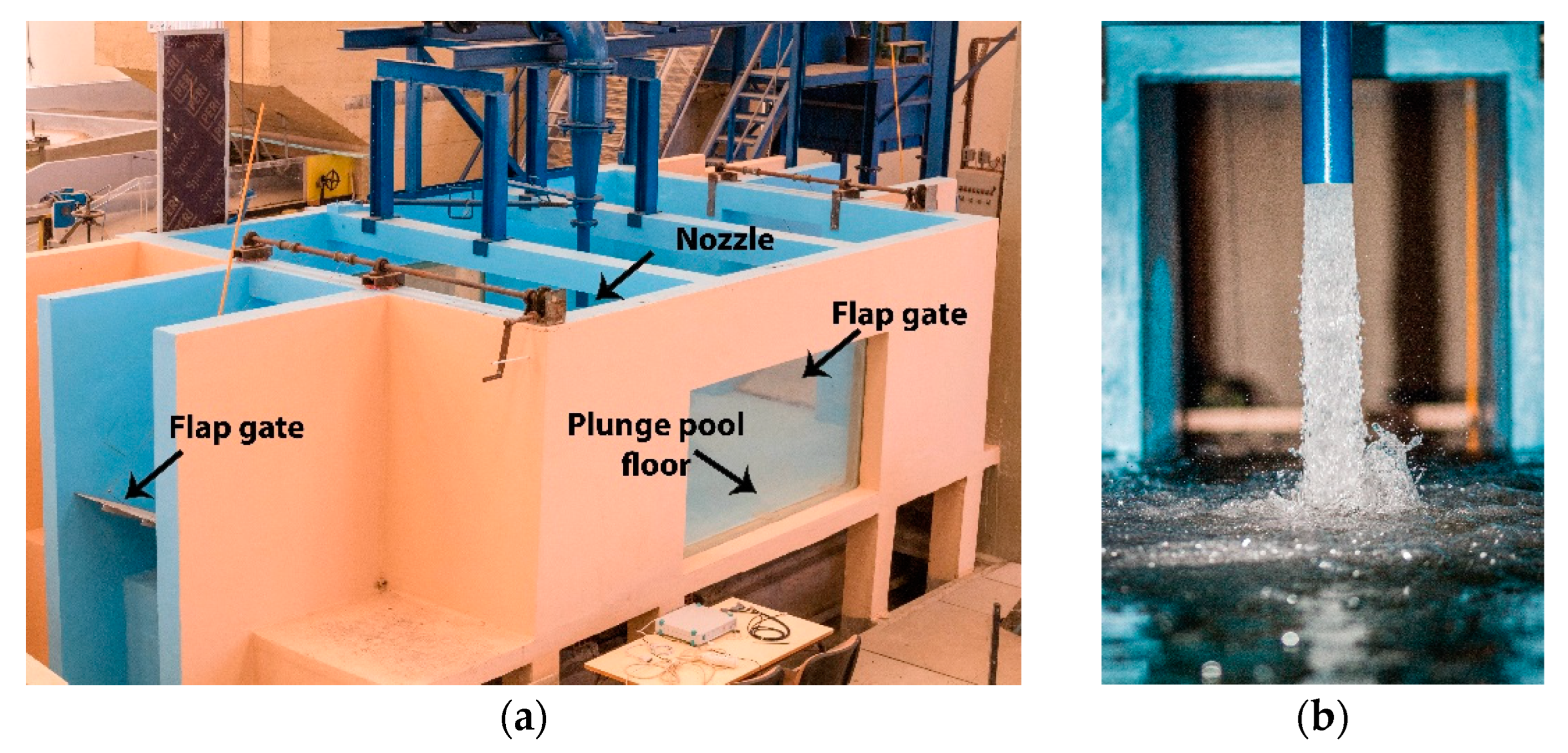
2.1. Experimental Setup

An experimental facility measuring 4.00 m in length and 2.35 m in width was constructed in the Hydraulics Department of LNEC and digitally reproduced for flow numerical analysis, as presented in the next section. This setup was specifically designed to generate vertical free-water jets with a maximum velocity of 18.0 m/s, as depicted in Figure 1a, from a 72 mm diameter nozzle, $D_i$, 1.00 m above the facility base (Figure 1b). The setup includes two flap gates, each 0.65 m wide, located 2.00 m from the jet axis along the longitudinal direction. These gates control water levels within the facility, ranging from 0.30 to 1.10 m, thus enabling the creation of both plunging and submerged jets, given that the maximum pool depth can submerge the nozzle exit [14].

The nozzle directs the jet flow vertically onto a 1.00 m × 1.00 m metallic plate equipped with pressure transducers. Figure 2 illustrates the placement of these sensors, with the projection of the nozzle cross-section marked with the green circumference. The pressure transducers are distributed within a single quadrant of the metallic plate based on the confirmed symmetry of pressure readings across all quadrants. This symmetry was verified through preliminary tests in which pressures were measured in the other three quadrants of the bottom plate. A total of nineteen transducers were deployed throughout the study at various locations. The dimensionless distance from the projection of the jet’s central point on the plate to the center of each sensor, $r/D_i$, varies from 0.25 to 4.51. Four transducers were intentionally placed near the jet stagnation point $r/D_i<0.50$, and two pairs with identical $r/D_i$ ratios (0.35 and 2.04) were positioned to further double-check for symmetry conditions during the testing procedure. The number of sensors positioned in the jet stagnation zone is relevant since this approach intends to address existing knowledge gaps regarding pressure levels in this area, where previous research has typically considered only one or two sensors in this zone [3,9,10,11].

Five Kulite XTM-190 (M)-17BAR-A transducers were arranged near the jet central axis (3.9 mm diameter, 17 bar range, and 1% accuracy), and fourteen ADZ Nagano SMF in the remaining measurement locations (25.4 mm diameter, 20 bar range, and 1% accuracy), as shown in Figure 2. The Kulite transducers were predominantly positioned near the jet axis to optimize measurement accuracy, as their diaphragm area is very small. The data acquisition system comprises three HBM Spider 8 data loggers controlled by a laptop. Measurements were acquired at acquisition frequencies between 600 Hz and 2400 Hz. The data series generated include 131,072 (2¹⁷) values for the 600 Hz acquisition frequency and 524,288 (2¹⁹) values for the 2400 Hz, spanning approximately 218 s of measurements. These dual frequencies were selected based on preliminary tests, which indicated that the 600 Hz frequency was insufficient for fully capturing the pressure spectrum at high velocities and lower pool depths [25].

2.2. Experimental Data

The experimental tests considered in this study are a subset of the experimental studies carried out and described by Jamet et al. [14]. For the hereby presented study, measured pressures for the jet with an issuance velocity $V_i=7.4 \mathrm{m}/\mathrm{s}$, and constant plunge pool depth Y = 0.8 m are considered. The experimental data of the air concentration and velocity data from other authors were used. Duarte [12,26] also performed measurements of air concentration and the velocity field for the same jet characteristics in an experimental facility with a 72 mm circular jet. Experimental results are plotted in charts against corresponding numerical results in the results section.

3. Numerical Modeling

3.1. Solver Comparison

Simulating a two-phase flow by solving the Navier-Stokes equations presents several challenges, including the modeling of air entrainment, coupling equations at the air-water interface, tracking the fluids interface, and addressing turbulence interactions between the phases [27]. The present study used two types of OpenFAOM solvers: an interfacial model, interFoam, and an Euler–Euler Model, twoPhaseEulerFoam [28].

InterFoam is a single-phase Euler model that solves the Navier-Stokes equations for two incompressible, isothermal, and immiscible fluids using the VoF method to track the fluids 1 and 2 interfaces, respectively water and air in this study [18,29,30,31]. The fluid density, $\mathsf{\rho }$, in each computational cell is calculated as $\mathsf{\rho }=\mathsf{\alpha }{\mathsf{\rho }}_1+(1-\mathsf{\alpha }){\mathsf{\rho }}_2$ where $\mathsf{\alpha }$ represents the fluid 1 volume fraction: $\mathsf{\alpha }=1$ if the cell is entirely filled with fluid 1, $\mathsf{\alpha }=0$ if the cell is filled with fluid 2. The governing mass and momentum equations are provided in Equations (1) and (2), respectively.

$$\nabla ·\overrightarrow{\mathrm{V}}=0$$

(1)

$${\displaystyle \frac{\partial \mathsf{\rho }\overrightarrow{V}}{\partial \mathrm{t}}}+\nabla ·\left(\mathsf{\rho }\overrightarrow{V}\overrightarrow{V}\right)=-\nabla {\mathrm{p}}_{-\mathrm{r}\mathrm{g}\mathrm{h}}-\overrightarrow{g}\overrightarrow{X}·\nabla \mathsf{\rho }+\nabla ·\left[2\left(\mathsf{\mu }+{\mathsf{\mu }}_t\right)S\right]+{\overrightarrow{\mathrm{F}}}_{\mathsf{\sigma }}$$

(2)

where: $\overrightarrow{V}$, denotes the velocity vector; $\mathrm{t}$, time; ${\mathrm{p}}_{-\mathrm{r}\mathrm{g}\mathrm{h}}=\mathrm{p}-\mathsf{\rho }\mathrm{g}\mathrm{h}$, alternative pressure term; $\mathrm{h}$, elevation; $\overrightarrow{g}$, gravitational acceleration vector; $\overrightarrow{X}$, position vector; $\mathsf{\mu }$, molecular dynamic viscosity; ${\mathsf{\mu }}_t$, turbulent dynamic viscosity; $S$, strain rate tensor, and ${\overrightarrow{\mathrm{F}}}_{\mathsf{\sigma }}$, surface tension. To prevent numerical diffusion and maintain a sharp interface, interFoam incorporates an artificial compression term in the VoF equation, involving a compression coefficient that can have values, typically, between 0 (no compression, i.e., interface undergoes significant numerical diffusion, becoming more stable) and 4 (maximum compression, sharp interface, risk of numerical instability. This term acts near the interface, counteracting numerical smearing by advecting the phase fraction along the interface normal. The present study uses a compression coefficient of 1, ensuring a good balance between interface sharpness and numerical stability.

The twoPhaseEulerFoam solver, an Euler–Euler type solver, was also employed in this study. This solver is suitable for solving two compressible, inter-penetrating phases. The continuity and momentum equations associated with this solver are presented in Equations (3) and (4) [18,32,33,34].

$${\displaystyle \frac{\mathsf{\delta }{\mathsf{\alpha }}_{\mathrm{d}}}{\mathsf{\delta }\mathrm{t}}}+\nabla ·\left({\mathsf{\alpha }}_{\mathrm{d}}{\mathsf{\alpha }}_{\mathrm{c}}{\overrightarrow{V}}_r\right)+\nabla ·\left({\mathsf{\alpha }}_{\mathrm{d}}\overrightarrow{V}\right)={\mathsf{\alpha }}_{\mathrm{d}}\nabla ·\overrightarrow{V}+{\mathsf{\alpha }}_{\mathrm{c}}\nabla ·{\overrightarrow{V}}_d-{\mathsf{\alpha }}_{\mathrm{d}}\nabla ·{\overrightarrow{V}}_c$$

(3)

$$\begin{gathered} {\displaystyle \frac{\mathsf{\delta }{\mathsf{\alpha }}_{\mathrm{\phi }}{\mathsf{\rho }}_{\mathrm{\phi }}{\overrightarrow{V}}_{\mathrm{\phi }}}{\mathsf{\delta }\mathrm{t}}}+\nabla ·\left({\mathsf{\alpha }}_{\mathrm{\phi },\mathrm{f}}{\mathsf{\rho }}_{\mathrm{\phi },\mathrm{f}}\overrightarrow{\varnothing }\overrightarrow{V_i}\right)-{\mathsf{\epsilon }}_{\mathrm{c}\mathrm{o}\mathrm{n}\mathrm{t},\mathrm{\phi }}\overrightarrow{V}+\left({\mathsf{\alpha }}_{\mathrm{\phi }}{\mathsf{\rho }}_{\mathrm{\phi }}+C_{vm}\right){\displaystyle \frac{\delta {\overrightarrow{V}}_{\mathrm{\phi }}}{\delta t}}= \\ =\nabla ·R^{eff}-C_d\overrightarrow{V}-C_{vm}\left({\displaystyle \frac{D{\overrightarrow{V}}_{\mathrm{\phi }}}{Dt}}-{\displaystyle \frac{D{\overrightarrow{V}}_{\mathsf{\beta }}}{Dt}}\right) \end{gathered}$$

(4)

where: subscript $c$ denotes the continuous phase; subscript $d$ denotes the disperse phase; $\mathsf{\alpha }$ represents the phase fraction; ${\overrightarrow{V}}_r$ is the relative velocity vector between the phases calculated based on ${\overrightarrow{V}}_r=\left({\overrightarrow{V}}_d-{\overrightarrow{V}}_c\right)+T_{D,d}+T_{D,c}$ where $V_d$ and $V_c$ are the dispersed and continuous phases, respectively; $T_{D,d}$ is the turbulent dispersion term for the disperse phase; $T_{D,c}$ is the turbulent dispersion term for the continuous phase; $\overrightarrow{\mathrm{\varnothing }}$ is the face-flux vector; ${\mathsf{\epsilon }}_{\mathrm{c}\mathrm{o}\mathrm{n}\mathrm{t},\mathrm{\phi }}$ represents the continuity error; $C_{vm}$ is the virtual mass coefficient; $C_d$ is the drag coefficient; ${\mathrm{R}}_{\mathrm{\phi }}^{-\mathrm{e}\mathrm{f}\mathrm{f}}$ is the effective stress rate sensor, Equation (5) where ${\nu }_{eff}$ is the effective viscosity, ${\nu }_{eff}=\nu +{\nu }_t$ and $k$ the turbulent kinetic energy.

$$R_{\mathrm{\phi }}^{eff}=\left[\nabla ·\left({\mathsf{\alpha }}_{\mathrm{\phi }}{\mathsf{\rho }}_{\mathrm{\phi }}{\nu }_{eff}\overrightarrow{V_{\mathrm{\phi }}}\right)-\left({\mathsf{\alpha }}_{\mathrm{\phi }}{\mathsf{\rho }}_{\mathrm{\phi }}{\nu }_{eff}\left(\nabla {\overrightarrow{V}}_{\mathrm{\phi }}^T-{\displaystyle \frac{2}{3}}\left(tr\nabla ·\overrightarrow{V_{\mathrm{\phi }}}\right)\right)\right)I\right]+{\mathsf{\alpha }}_{\mathrm{\phi }}{\mathsf{\rho }}_{\mathrm{\phi }}{\displaystyle \frac{2}{3}}{k}_{\mathrm{\phi }}I$$

(5)

A major limitation of the interFoam solver is its inability to effectively simulate small water droplets, as their generation depends on the mesh size [23,27]. In practical civil engineering applications, simulating large-scale spillways is infeasible due to the requirement for very fine meshes to accurately represent water droplets with millimeter-scale diameters. In contrast, the twoPhaseEulerFoam solver can model two distinct fluid phases and account for mass transfer between them.

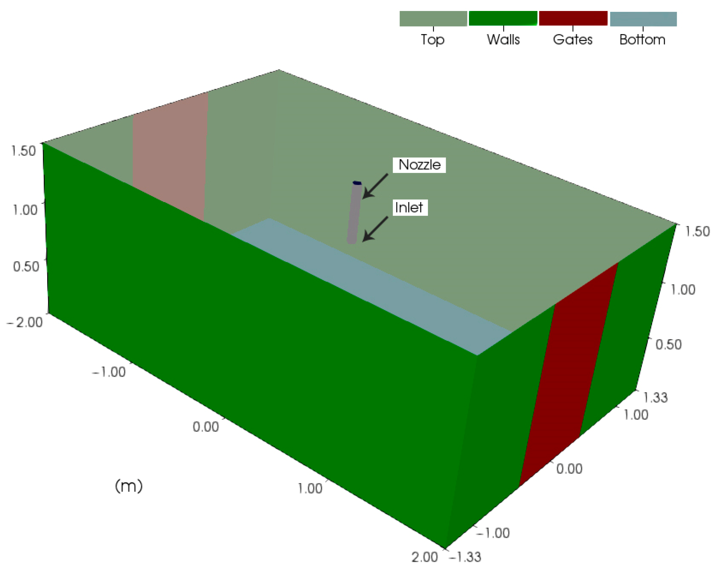
3.2. Numerical Domain, Boundary Conditions, and Numerical Schemes

A numerical domain was defined to replicate the flow conditions of the experimental facility, as shown in Figure 3. The domain dimensions are 4.00 m × 2.65 m × 1.50 m, matching those of the experimental setup. Similar to the experimental facility, a 72 mm circular inlet is located 1.00 m above the bottom of the domain. The only difference between the two setups is how the outlet boundary condition is imposed. Instead of reproducing the flap gates considered in the experimental facility, in the numerical model, the outlet boundary condition was set up as detailed below to allow the simulation of different pool depths without a need for mesh adjustments that the simulation of the flap gates would require.

The boundary conditions were closely defined to match those of the experimental facility and were consistently applied to allow direct comparison with the results from each solver.

The top part of the domain was kept open to atmospheric pressure for all variables, while the walls and bottom were treated as natural surfaces with a fixed velocity of zero. Wall functions were applied in the turbulent kinetic energy and dissipation fields, and a roughness wall function was used to simulate wall roughness.

A fixed velocity corresponding to the specified inlet velocity was applied to the inlet. Since only water entered the domain, the water volume fraction was set to one. Turbulent kinetic energy was defined based on turbulence intensity, which was determined through a sensitivity analysis. The selected range of values was derived from experimental measurements of turbulence intensity [4,10,35].

Two gates represented the model outlets. To model this scenario, a wave absorption boundary condition was implemented to maintain a constant water level in the model of 0.8 m [36].

The Reynolds-Averaged Navier-Stokes (RANS) k-Omega SST model was used in both solvers to characterize flow turbulence. This two-equation model assumes that Reynolds stresses are proportional to the mean velocity gradients [37,38]. Castillo et al. [19,21] concluded that the k-Omega SST model provided the best agreement between experimental and numerical results in an impinging jet. Similarly, Mendes et al. [17,18] observed a better agreement between numerical and experimental results when simulating a water jet and a spillway aerator with the k-Omega SST model. The k-Epsilon turbulence model was not used, as it produced unstable results in the preliminary simulations when coupled with the turbulent dispersion model in the twoPhaseEulerFoam solver.

The twoPhaseEulerFoam solver can couple a turbulent dispersion model with the general flow model. Three different models were evaluated: Lopez [39], Burns [40], and Gosman [41]. Preliminary tests were conducted to determine the most suitable model. The Burns model was discarded due to numerical instability, while the Lopez and Gosman models produced similar flow conditions. The Lopez model was ultimately selected for its lower computational effort compared to the Gosman model.

For numerical schemes, an Euler implicit time scheme was employed for time discretization, and a Gauss linear upwind scheme was applied for the divergence of velocity, k, and omega. Flow characteristics from the numerical simulations were obtained after an initial simulation period to ensure time independence of the water volume in the domain, and the values of the total kinetic and turbulent kinetic energies were also time independent.

The simulations were performed on an HPC cluster featuring Intel Xeon E5-2680 (2.70 GHz) processors, each with 16 cores. The number of cells per processor remained constant for the first three meshes. However, for the most refined mesh, the number of cells assigned to each processor increased due to limitations on the number of processors. This constraint led to significantly longer computation times.

3.3. Mesh

Four different meshes with cubic cells were utilized in the simulations. Mesh 1 serves as the reference, while the other three are sequential refinements in the region of interest, focusing on the jet and considering a pool depth of 0.8 m. Figure 4 shows a cross-section by the axis illustrating the different meshes. All meshes maintain a constant cell size of 50.0 mm in the air far-field. Below the water surface, a cell size of 12.0 mm was applied in regions distant from the zone of interest. Near the nozzle, cell sizes range from 12.0 mm in Mesh 1 to 1.5 mm in Mesh 4.

Mesh 1 features a uniform cell size of 12.0 mm throughout all water domains, represented by the black line in Figure 4, corresponding to 6 cells across the jet diameter (D6), resulting in 5.0 million cells.

Mesh 2 introduces a refinement zone near the jet axis, indicated by the green line, with cells measuring 6.0 mm. This refinement increases the resolution to 12 cells across the jet diameter (D12), bringing the total to 6.7 million cells.

Mesh 3 incorporates three levels of refinement, resulting in 24 cells across the jet diameter (D24). The smallest cells, shown by the red line, measure 3.0 mm, with 19.0 million cells.

Mesh 4, the most detailed configuration, features 36 cells across the jet diameter (D36) and a cell size of 1.5 mm near the jet (indicated by the orange line). This setup leads to 58.6 million cells across the entire model of the experimental facility.

At this stage, a symmetry case was also tested. Three symmetry meshes were used: half of the experimental facility, a quarter, and an edge. The analyses of the flow characteristics lead to differences in the pressure at the plunge pool bottom and in the air concentration values along the pool depth. Due to that, this type of domain was discarded.

4. Results

4.1. Mesh Sensitivity Analysis

Preliminary results were analyzed using the four different meshes and the two methods to evaluate mesh dependency and the main differences between the models. The analysis focused on pressure at the plunge pool bottom, velocity, and air concentration within the plunge pool.

4.1.1. Dynamic Mean Pressure and Cell Size

The mean dynamic pressure is defined as the total pressure subtracted from the hydrostatic pressure given by the poll height. The results at the impact point $r/D_i=0.00$ are presented in Figure 5a, which shows the relationship between the number of cells in the jet cross-section for all four different meshes.

The analysis of Figure 5 shows that the mean dynamic pressure values produced by the twoPhaseEulerFoam solver are independent of the mesh resolution when the mesh consists of more than 24 cells in the jet diameter. In contrast, the interFoam solver exhibited mesh dependence, with the mean dynamic pressure increasing as the mesh was refined. When comparing the numerical results with the experimental data collected at the same location under identical conditions, it was found that the mean dynamic pressure obtained from the twoPhaseEulerFoam solver closely matched the experimental data for meshes with over 24 cells in the jet diameter, outperforming the results from interFoam. The interFoam solver, however, overestimated the pressures at the stagnation point.

For data obtained far from the stagnation point, $r/D_i=0.69$ (Figure 5b), both solvers showed mesh independence when more than 12 cells were considered in the jet diameter. The numerical results for $r/D_i>0.50$ displayed a good correlation with experimental results, even with coarser meshes (D12), when using the twoPhaseEulerFoam solver. However, the interFoam-VoF solver continued to overestimate the mean dynamic pressures.

4.1.2. Velocity and Cell Size

Considering the pressure and mesh dependency findings only results from meshes D24 and D36 are presented for both numerical models with a turbulent intensity in the inlet of 5%. The calibration of this value is present in Section 4.4. The numerical outputs of the mean velocity in the shear stress region can be directly compared with the published experimental results from Duarte [12,26]. In Figure 6, the non-dimensional velocity patterns with respect to the impact velocity in the plunge pool, $V_j$, expressed as functions of the ratios $z/D_i$ and $r/D_i$ where $z$ represents the distance from the water surface to the bottom, are shown.

Results evidence mesh independence for both solvers, and no significant differences were observed when comparing the outcomes of the two solvers. However, the numerical results did not accurately reproduce the velocity field observed in Duarte’s experimental data. Specifically, the numerical simulations failed to replicate the negative velocities in the experimental data outside the jet core.

4.1.3. Air Concentration and Cell Size

The air concentration near the impact point was analyzed as part of the mesh dependency analysis. Figure 7 illustrates the air concentration results obtained from the two models compared to the number of cells in the jet cross-section, along with experimental data collected by Duarte [12].

In Figure 7a, which shows the air concentration at r = 0.05 m and z = 0.20 m, it is clear that mesh refinement does not significantly affect the twoPhaseEulerFoam solver. Its results are close to the measurements taken by Duarte [12]. Conversely, the interFoam solver exhibits a substantial mesh dependency due to the limitations of the VoF model. For meshes with more than 24 cells in the jet diameter, the air concentration values from this solver drop to zero. Figure 7b shows a similar trend for both solvers at r = 0.10 m and z = 0.20 m.

Overall, when comparing the numerical results with the experimental data, it becomes evident that the twoPhaseEulerFoam solver provides closer values to the experimental measurements.

4.2. Mesh and Model Selection

4.2.1. Mesh

The results from the twoPhaseEulerFoam solvers for the D24 and D36 meshes were nearly identical, requiring a choice between them for subsequent simulations. Figure 5a presents the computation time per simulated second, T (in h/s), to evaluate the computational costs. It is evident that the D36 mesh requires approximately eight times longer to simulate one second than the D24 mesh. Consequently, the D24 mesh was selected for this study as it offered a more efficient balance between computational cost and accuracy.

The preliminary simulations revealed notable differences between the two models concerning mesh independence, requiring a decision on which solver to employ in subsequent simulations.

4.2.2. Pressure Comparison

The interFoam solver failed to achieve mesh-independent results across the four tested meshes. Figure 5a illustrates that within the jet stagnation point, twoPhaseEulerFoam demonstrated superior performance, yielding numerical results closer to experimental data, while interFoam consistently overestimated pressures. However, for pressures far from the jet stagnation point $r/D_i>0.69$, as shown in Figure 5b, interFoam provided good results. Notably, twoPhaseEulerFoam reached experimental pressure values with coarser meshes, reducing computational costs, as both solvers required the same time to compute one second of simulation duration.

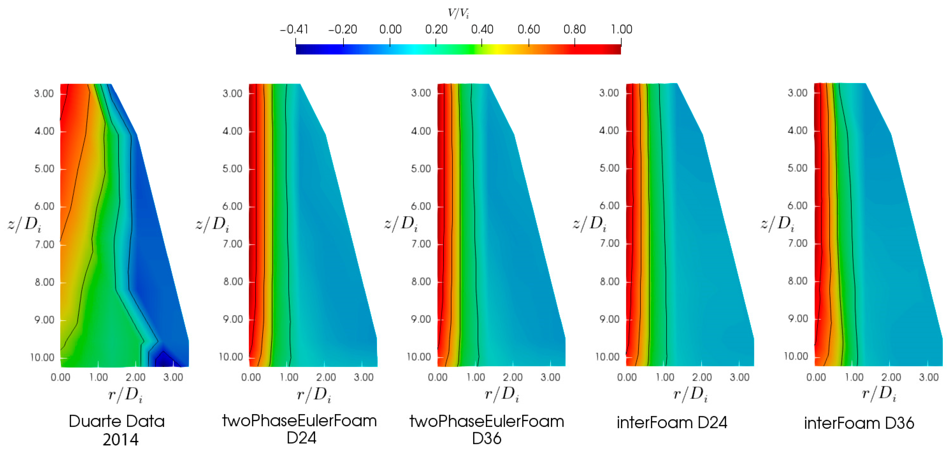
4.2.3. Velocity Field Analysis

The jet’s shear stress zone’s velocity pattern exhibited higher numerical values than experimental data, considering an initial turbulence intensity of 5% at the jet inlet section. When analyzing velocity decay along the jet’s centerline, both solvers maintained a coherent jet core over a distance that appeared mesh-independent. Comparisons indicate that the numerical results align more closely with findings from prior experimental studies, although both solvers overestimate velocities relative to experimental data.

4.2.4. Air Concentration Analysis

Simulating water-air mixtures is critical in hydraulic studies [27,42]. The solvers differ significantly in this regard: interFoam uses a VoF approach, while the twoPhaseEulerFoam adopts an Euler–Euler process [16]. Due to the methodological differences, interFoam air concentration results are highly sensitive to mesh resolution, as depicted in Figure 7 [43]. For example, at a point located 0.20 m above the surface and 0.10 m from the jet centerline, air concentration drops from 0.50 to 0.00 as mesh resolution increases from D6 to D24 (Figure 7b). In contrast, twoPhaseEulerFoam is less affected by mesh quality, producing results more consistent with Duarte’s experimental findings [12].

4.3. Boundary Layer Influence

Simulations were conducted exclusively using the twoPhaseEulerFoam solver to assess the influence of boundary layers. Wall functions were applied at the domain boundaries to model turbulence fields. Three boundary layers were tested, each with a maximum height of 3 mm, corresponding to the minimum cell height in the D24 mesh. An expansion ratio of 1.1 was used to define the height decay of successive cells. These boundary layers consisted of 4, 8 and 16 cells, and all tests were based on the D24 mesh.

Table 1. Mean dynamic pressure differences between original mesh and meshes with boundary layers.

$\mathit{r}/{\mathit{D}}_{\mathit{i}}$ (-)	Number of Cells in the Boundary Layer
	4	8	16
0.00	−1.0%	4.2%	−1.9%
0.25	−2.4%	2.7%	−1.5%
0.35	−3.2%	1.4%	−1.6%
0.69	−0.1%	−1.2%	−1.3%
1.04	0.3%	−2.1%	−0.8%

summarizes the differences in mean dynamic pressure at five distinct locations for meshes with and without boundary layers. The maximum observed difference was less than 4.2%, and no correlation emerged between the number of boundary layer cells and pressure variations.

Y+ values were analyzed at the bottom boundary to evaluate boundary layer effects further. These values, which depend on the distance from the jet’s centerline, reflect the flow’s complex behavior. For the D24 mesh without a boundary layer, y+ values measured ranged from 30 to 200 in the jet centerline to $r/D_i=0.15$, and for $r/D_i>10.0$. Introducing a 16-cell boundary layer reduced the maximum y+ value to around 170 near the jet but maintained values above 30 in regions far from it. Similar y+ trends were observed in all meshes with boundary layers for distances beyond $r/D_i=10.0.$

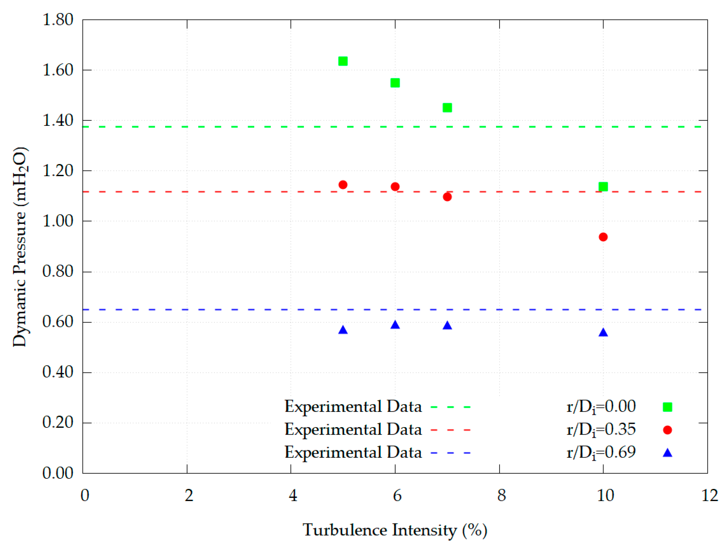
4.4. Initial Turbulent Conditions

The initial turbulent conditions are a critical factor influencing jet behavior during its air trajectory and dissipation in a plunge pool [4,11]. In experimental studies, this is quantified by the turbulence intensity, $T_i$. In numerical simulations, it is represented by the initial turbulent kinetic energy, $k$, and the dissipation rate, $\omega$.

In the present numerical simulations, turbulent kinetic energy was defined as a function of turbulence intensity, as described in Equation (6), where $\overrightarrow{V}$ represents the velocity magnitude at each cell. The dissipation rate was defined as a function of turbulent kinetic energy and the mixing length, $L$, as indicated in Equation (7). Here, $C_{\mu }$, an empirical constant was set to 0.09, and the mixing length was defined as ${0.07D}_i$.

$$k={\displaystyle \frac{3}{2}}{\left(T_i\overrightarrow{V}\right)}^2$$

(6)

$$\omega ={\displaystyle \frac{\sqrt{k}}{C_{\mu }^{0.25}L}}$$

(7)

Simulations were conducted using four different turbulence intensity values to assess the impact of inlet turbulence intensity. The results were compared with experimental data, as illustrated in Figure 8. The analysis indicated that a turbulence intensity of 7% provided the best match with the experimental results across all measurement points.

As expected, higher turbulence intensities led to lower bottom pressures due to increased turbulent kinetic energy, which enhances energy dissipation in the plunge pool. When comparing the mean dynamic pressure along the jet centerline for simulations with turbulence intensities of 10% and 5%, a difference exceeding 26% was observed. However, these discrepancies were less pronounced far from the jet stagnation point, $r/D_i>0.50$.

Further work on this topic is underway, involving a detailed 3D CFD simulation of the flow along the upstream pipe system to assess whether the jet’s initial turbulence and velocity conditions at a pipe section far upstream of the nozzle influence the resulting jet velocity profile and turbulence intensity.

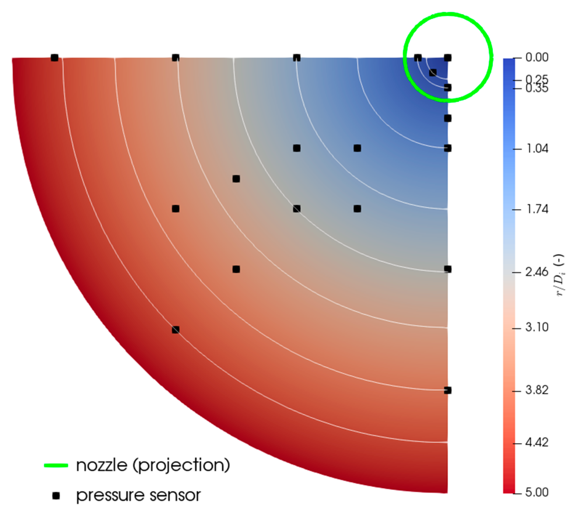
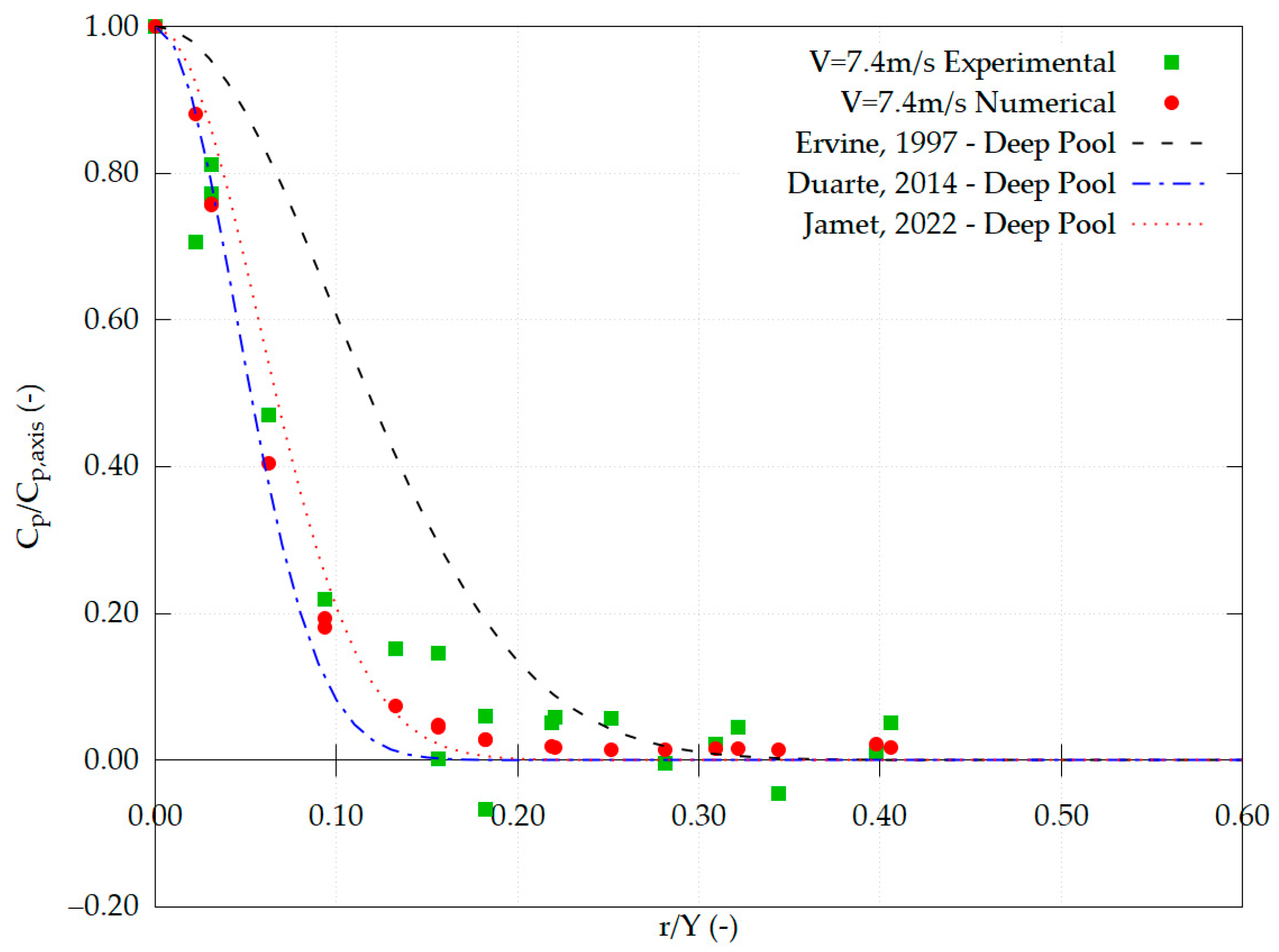
4.5. Dynamic Mean Pressure Distribution

Following the results from the preliminary simulation, in the following sections, the results presented are for the Euler–Euler model with a D24 mesh without a boundary layer and an initial turbulence intensity of 7%.

The analysis focused on the dynamic pressure near the stagnation zone, $r/D_i<0.50$. The numerical data closely matched the experimental results, with discrepancies of less than 5% for pressure transducers located along the jet centerline and at $r/D_i=0.35$ (Figure 9). However, a significant deviation was observed at $r/D_i=0.25$, where the recorded mean dynamic pressure did not conform to a theoretical Gaussian curve distribution, resulting in notable differences between the numerical and experimental data.

Outside the stagnation zone, the numerical results aligned well with the experimental findings, exhibiting only minor differences.

Figure 10 presents the dimensionless variation of the mean dynamic pressure coefficient, normalized by its axis value, as a function of the distance from the jet stagnation point divided by the pool depth. Ervine et al. [3] proposed an equation for this dimensionless variation, suggesting values of $K_2$ equal to 30 for shallow pool depths ($Y/D_j<4.0$) and 50 for deep pool depths, based on data from five pressure transducers within $r/Y<0.3$, Equation (8).

$${\displaystyle \frac{C_p}{C_{p,axis}}}=e^{-K_2{\left({\displaystyle \frac{r}{Y}}\right)}^2}$$

(8)

The dimensionless mean dynamic pressure coefficient, $C_p$, is defined in Equation (9), where $p_{mean}$ represents the time-averaged dynamic pressure, Y the pool depth, and $\Phi$ a correction factor for non-uniform nozzle exit velocity distribution. Analyzing dynamic pressure during tests with a jet velocity of 7.4 m/s and pool depths between 0.3 m and 0.9 m, a correction factor value of 1.083 was derived. Similar values have been noted in simulations of high-velocity water jets in analogous experimental setups [10,11].

$$C_p={\displaystyle \frac{p_{mean}-Y}{\Phi \raisebox{1ex}{$V_j^2$}\!\left/ \!\raisebox{-1ex}{$2g$}\right.}}$$

(9)

Duarte [12] proposed values of 25 for shallow pools ($Y/D_j=4.2$) and 250 for deep pools ($Y/D_j=11.1$), based on results from four pressure transducers at $r/Y<0.1$. In this study, data from nineteen pressure transducers positioned up to $r/Y=0.41$ confirmed a pool depth of 0.8 m as corresponding to a deep pool ($Y/D_j=11.11$). The numerical and experimental results better matched Duarte’s values for deep pools. Furthermore, Jamet et al. [14], analyzing data from five sensors near the jet stagnation point during the same experimental campaign, proposed a curve that closely fits the present results from numerical modeling.

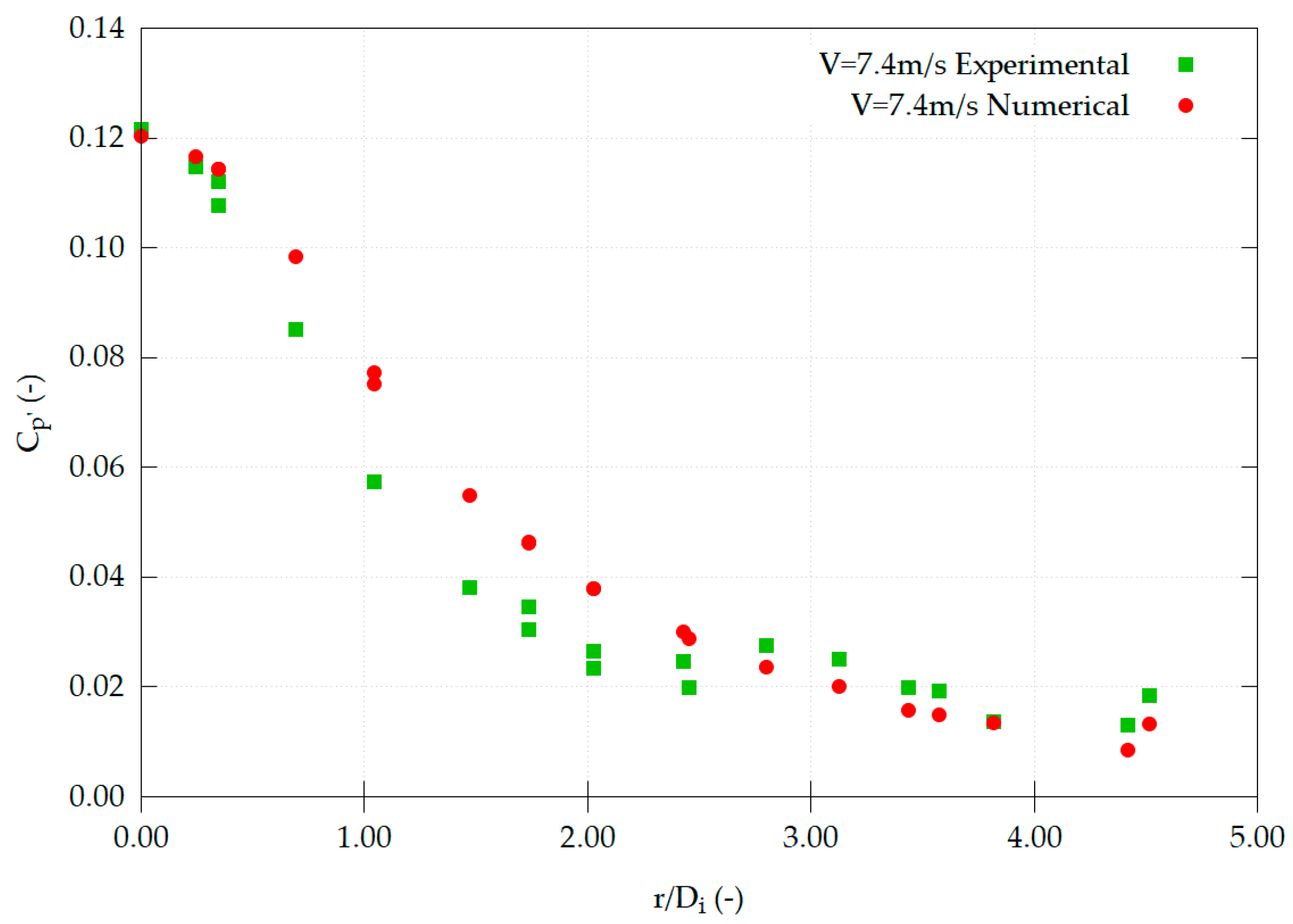
4.6. Turbulent Component of the Pressure

Pressure fluctuations remain a critical area of study, primarily due to the computational challenges associated with performing LES for these types of flows. This study assessed the twoPhaseEulerFoam solver’s capability in simulating the pressure’s turbulent component. When coupled with the k-OmegaSST turbulence model, the solver cannot simulate pressure fluctuations, highlighting a significant limitation of solvers using Reynolds-Averaged Navier–Stokes (RANS) turbulence models.

If this type of turbulence model, RANS, is applied, regardless of the numerical schemes for computing time, pressure, and velocity evolution in time, we can easily find out that results in terms of fluctuations will remain unchanged, i.e., are not captured by the model because the numerical simulation reaches a semi-steady state. Experimental studies express the fluctuating dynamic pressures by a coefficient, $C_{p^{\prime }}$, defined in Equation (10), where $\sigma$ represents the standard deviation of the pressure. Since the numerically calculated pressures with RANS are steady, the resulting standard deviation, $\sigma$, equals zero.

This shortcoming of the RANS turbulence model was overcome by applying the empirically deduced Equation (11) proposed by Ervine et al. [3].

$$C_{p^{\prime }}={\displaystyle \frac{\sigma }{\Phi \raisebox{1ex}{$V_j^2$}\!\left/ \!\raisebox{-1ex}{$2g$}\right.}}$$

(10)

$$C_{p^{\prime }}=10{\left({\displaystyle \frac{u^{\prime }}{U_j}}\right)}^2$$

(11)

As the turbulence model calculates the turbulent kinetic energy $k$, which is in itself a measure of the turbulent fluctuating parameters of the flow, one can compute the root mean square of the velocity fluctuations, denoted as $u^{\prime }$, from the turbulent kinetic energy using Equation (12).

$$u^{\prime }=\sqrt{{\displaystyle \frac{2k}{3}}}$$

(12)

Figure 11 presents the fluctuating dynamic pressure coefficient, $C_{p^{\prime }}$, as a function of $r/D_i$. In a simulation involving a 7.4 m/s jet in a plunge pool with a water depth of 0.8 m, the pressure fluctuations estimated through Equation (11) aligned closely with the experimental data within the jet stagnation point. Discrepancies between numerical and experimental data were minimal.

However, as the measuring point moves away from the jet stagnation point ($r/D_i>0.69$), numerical simulations predicted more intense pressure fluctuations than experimentally observed. Conversely, at distances farther from the jet centerline ($r/D_i>2.80$), experimental data revealed higher fluctuating dynamic pressure coefficients than numerical estimates.

4.7. Jet Centerline Velocity

The mean jet centerline velocity profile, from the jet’s initial section to the bottom with an inlet turbulent intensity of 7%, is illustrated in Figure 12. The profile reveals three distinct flow regions: the flow development zone—the jet maintains its core velocity equal to the velocity at the impact point; the flow established zone—the jet centerline velocity decreases linearly with distance; and finally, the impingement zone—the influence of the pool bottom alters the velocity field [1,3,4].

The velocity slope in the impingement zone from the numerical simulations aligned closely with the results of Giralt et al. [44], who studied air jets impinging on aluminum plates at various distances. Under similar jet conditions ($V_i=7.4 \mathrm{m}/\mathrm{s}$, at Y = 0.8 m), Duarte [12] measured the velocity of the air bubbles in the jet and assumed that water particles shared the same velocity. A comparison revealed that Duarte’s experimental velocities were consistently lower than the numerical results at most points, except for the last point near the plunge pool bottom.

5. Discussion

5.1. Preliminary Results and Mesh Sensitivity Analysis

Regarding mesh sensitivity, the analysis performed in the preliminary results of the interFoam solver did not reach mesh independence for pressure near the stagnation point, and the values of the pressure obtained were higher than those of the experimental ones. This fact can lead to the conclusion that the interfacial VoF model cannot reproduce the diffusion caused by the shear stress inside the plunge pool due to the impossibility of the simulated fluids changing energy between them. On the other side, the Euler–Euler model has one set of equations for each fluid and is more capable of simulating the energy changes between the fluid phases. Looking for the variation of the mean dynamic pressure as a function of the cell size, it is possible to verify that the values obtained by the interFoam solver increase with every new refinement, and no diffusion in the jet is simulated.

On the other hand, because this model does not have mesh independence, the value of the mean dynamic pressure can be closer to the experimental ones for coarser meshes with cell dimensions that cannot describe the flow patterns correctly. By opposition, the Euler–Euler solver tends to a constant value of the mean dynamic pressure as the cell size is reduced. The obtained values also fit the experimental data. Outside of the jet footprint, both solvers reach mesh independence, but in the same way, the solver that better matches the experimental data is the Euler–Euler one. The interfacial VoF model continues to overestimate the pressures due to the inefficient jet diffusion.

A good compromise between computation time and results quality is achieved with the D24 mesh at the stagnation zone. Similar findings were reported by Mendes et al. [42] and Maleki et al. [23], who concluded that an optimal trade-off between mesh resolution and simulation accuracy could be achieved with comparable mesh densities. Furthermore, Mendes et al. [17] noted that mesh independence was only achieved with the twoPhaseEulerFoam solver. Regarding time consumption, D36 mesh leads to simulations taking eight times more time than the simulation with twenty-four cells in the jet diameter.

The flow velocity inside the plunge pool leads to mesh independence in both numerical approaches. The simulated core lengths exceed the experimental measurements by more than threefold. Furthermore, the core penetration observed in the simulations was significantly higher than that in Duarte’s data, with experimental results indicating a core penetration of approximately ${3.5D}_i$. Like the mean dynamic pressure, the initial jet turbulence conditions strongly influence the velocity field at this stage of the preliminary tests. This variable has not yet been calibrated; due to that, the velocity values are higher than the experimental ones.

In terms of the air concentration inside the plunge pool, the twoPhaseEulerFoam solver showed minimal mesh dependency, while interFoam results varied significantly, with air concentration values ranging from 0.5 to 0.0 when comparing the D6 results to those from other finer meshes. This is one of the significant limitations of the interfacial VoF model. The simulation of water droplets when simulating a free-water jet is related to the cell size due to changes in these variables, leading to significant differences in air concentration values [23,27]. InterFoam solver is more capable of simulating separated flows due to the inability to simulate fluid mixing. The fluid mixture is simulated in this model due to numerical diffusion, which can be notable in meshes with lower cell resolutions. On the other side, we have the Euler–Euler model, where two distinct fluid phases are calculated, and the mixing between them can be modeled.

The following main conclusions were drawn from this analysis:

• Pressure and air concentration: TwoPhaseEulerFoam accurately reproduces stagnation point pressures and air concentrations.
• Velocity field: Both methodologies predict higher velocity fields than experimental data, but these estimates are consistent with prior research.
• Computational efficiency: Given similar computational costs, twoPhaseEulerFoam lower sensitivity to mesh quality allows for coarser meshes, reducing computational expenses without compromising accuracy.

The evaluation of the boundary layer influence in the dynamic pressures at the plunge pool led to more extended simulations without a significant increment in the quality of the results. The mesh with 16 cells on the boundary layer required 2.2 times longer simulation time than the D24 mesh without a boundary layer. The obtained pressure values do not follow a trend as the boundary layer has more layers. The mean dynamic pressure reduction observed in the meshes with 4 and 16 cells in the boundary layer can directly relate to the capacity to simulate the velocity patterns near the bottom. Given the minimal differences in pressure field predictions and the implementation of wall functions at the domain’s bottom and side walls, it was concluded that boundary layers were unnecessary for this study.

Manso [11] performed pressure fluctuation measurements at the insure section of a jet with the same diameter and obtained a value below 8% for jets with initial velocities lower than 12 m/s. Older studies of McKeogh and Elsawy [45] obtained values of turbulence intensity of 2% for turbulent jets with velocities lower than 5 m/s. May and Willoughby [6] performed measurements with a total-head Pitot tube, a value between 5.5 and 5.8% of turbulence intensity for jets with velocities from 4.9 m/s and 6.6 m/s. Using a laser Doppler velocimeter, Ervine and Falvey [4] obtained a value of 5% for rough turbulent plunging jets with velocities in the 3.3 to 29.0 m/s range. The initial turbulence intensity sensitivity analysis performed in the present study led to a value of 7% at the jet initial section, which better fit the experimental data. Looking for the values in the literature, it is possible to verify that flow characteristics depend on the type of experimental facility where it is measured. However, the numerical obtained value is in the range of the values measured in experimental facilities by other authors.

5.2. Flow Characteristics of a 7.4 m/s Jet Impinging into a Plunge Pool with a Pool Depth of 0.8 m

The pressure distribution at the bottom of the plunge pool reveals a good agreement between experimental and numerical data. However, some differences were noticed. These discrepancies can be attributed to how the hydrostatic pressure, which corresponds to the pool depth, was defined for each data series. In the experimental tests, uncertainties arise due to plunge pool free surface oscillations and measuring equipment limitations, with only one measurement location used to read the pool depth. Similarly, the numerical model assumed a constant pool depth of 0.8 m, replicating the measuring system of the experimental facility. Both methods potentially introduced errors significantly further from the jet centerline, where total pressure approaches the hydrostatic pressure associated with the pool depth. During the experimental tests, oscillatory movements of the diffusing jet relative to its theoretical axis were observed, leading to an oscillation of the actual stagnation point relative to the theoretical one. This oscillatory phenomenon, resulting from experimental constraints, does not occur in the numerical modeling of jet diffusion and is one of the main causes of differences in the respective pressure fields near the jet impact zone. Another relevant factor influencing the pressure field at the plunge pool bottom is the air entrainment conditions occurring at the pool free-surface impingement section, which significantly affects jet diffusion and associated energy dissipation. Since no measurements have yet been obtained in the experimental facility regarding this local phenomenon, it is not yet possible to compare and validate the accuracy of the numerically computed air entrainment at this location. Looking for the mean dynamic pressure coefficient divided by the mean dynamic pressure coefficient at the axis, the numerical results fit well with data from the experimental campaign performed by other authors. The curve that better fits the numerical data is the one proposed by Jamet et al. [14]. This was expected once the experimental data used to fit the curve was the same as in the present study. The difference between the numerical data and the fitted curve can be explained by the fact that Jamet only uses five pressure sensors, two at the same distance to the jet central line. Due to this, the proposed curve can be narrower due to the limited range of sensor distances to the jet stagnation point. Comparing numerical results with experimental data under similar flow conditions and findings from other studies confirm that the numerical simulations accurately replicated the dynamic mean pressure at the bottom of the pool.

The numerical simulation of the fluctuation component of the pressure field is now an open topic in the literature. The Euler–Euler model coupled with the K-Omega SST turbulent model cannot reproduce the pressure fluctuations. Due to that, a possible way to obtain that pressure component is to use large eddy simulation (LES) or detached eddy simulation (DES). The main difference between these two is that in the DES models, the turbulence scales were simulated using LES up to a certain turbulence scale. From the moment the cell size cannot reproduce the smaller turbulent scales, a RANS model is applied. The main advantage of this model type is the capacity to simulate part of the turbulent eddies without the need for a very fine mesh in the zones near the walls. An assessment of the mesh resolution to use LES or DES based on the flow characteristics obtained using the k-Omega SST model was performed, and mesh resolutions higher than D36 were needed. Additionally, the computation costs of using a finer mesh than the D36 are eight times slower than the D24 mesh. Therefore, it is impossible to use these types of turbulent models in this type of simulation. Performing simulations with the DES K-OmegaSST model using the D24 mesh can lead to some pressure fluctuations, but the simulation time increases by 2.75 times, which is a need of 1.5 days to perform one second of simulation. A simulation with some seconds was needed to obtain statistical moments from the pressure signal. In practical engineering cases, a way to have numerical results for so long is incompatible with the deadlines of design phases. A significant limitation of using this type of method is the impossibility of using a curser mesh to start new simulations. This leads to the initial time of simulation, which must be used to stabilize the flow conditions before obtaining the pressure signal. Due to this, the simulation time will increase significantly. By applying the relation between the velocity fluctuations and the mean pressure coefficient proposed by Ervine et al. [3], Equation (11) produced a good agreement between the two data sets. Numerical results fit well the pressure fluctuation coefficient at the zone near the jet stagnation point, far from this region; $r/D_i>0.69$, the numerical fluctuations are higher than the experimental ones. Then, at distances far from the jet centerline ($r/D_i>2.80$), the obtained experimental and numerical values are very close. Bollaert [10] relates the pressure fluctuation at this region to the air concentration at the plunge pool bottom. The air concentration values at the bottom of the plunge pool are directly related to the jet air concentration at the impinging section of the plunge pool and the additional volume of air that locally enters that location. It must be pointed out when comparing experimental and numerical results that the experimental approach for measuring the pressure fluctuations involves several uncertain sources, particularly due to the inherent errors associated with the measurement chain, starting on the fact that the transducers, although very small, have physical dimensions. The numerical model also involves mesh-induced errors, boundary condition limitations and empirically estimated parameters. Despite the efforts to minimize these aspects, they are among the causes of observed differences between experimental and numerical results.

The jet velocity profile obtained in the numerical simulations reveals a core persisted for ${5.0D}_i$ when a turbulent intensity of 7% is used at the jet’s initial section. For reference, Ervine and Falvey [4] observed core lengths of ${4.0D}_i$ for circular plunging water jets with Reynolds numbers of 10⁵ to 10⁶. Albertson et al. [46] and Beltaos and Rajaratnam [47] reported core lengths between 6.2 to ${6.8D}_i$ for air jets with Reynolds numbers exceeding 1500, while Duarte [12] proposed a maximum core length of ${7.8D}_i$ for high-velocity flows. Despite these differences, the established flow zone showed a consistent velocity decrease slope when compared with Giralt et al. [44]. The analysis of the initial turbulent conditions confirms that the jet’s initial state significantly affects the pressure and velocity fields. Consequently, direct comparisons with experimental data from other studies are challenging, as the initial turbulence conditions are not explicitly presented in those studies.

Further research is needed to enhance solver capabilities, particularly in (i) expanding the range of jet velocities and pool depths by simulating additional scenarios that can be directly compared with experimental data, (ii) improving the simulation of jet diffusion under shear flow dominating conditions, (iii) enhancing the accuracy of pressure fluctuations predictions, and (iv) applying twoPhaseEulerFoam to other hydraulic structures for broader validation.

6. Conclusions

This study evaluated the performance of numerical simulations in replicating the behavior of a high-velocity free-water jet ($V_i=7.4 \mathrm{m}/\mathrm{s}$) impacting a plunge pool (Y = 0.8 m). Two solvers, interFoam (VoF approach) and twoPhaseEulerFoam (Euler–Euler approach), were tested. Results were compared against experimental data collected at LNEC, where pressures were measured at 19 locations with acquisition rates of 600 Hz.

(A) Solver comparison and key findings

Mesh resolutions: TwoPhaseEulerFoam demonstrated mesh independence for mean dynamic pressure and air concentration, while interFoam showed mesh dependency, especially at the jet stagnation point. The following additional conclusions are pointed out:

• Different mesh resolutions were tested and labeled as D6, D12, D24, and D36, corresponding to meshes containing 6, 12, 24, and 36 cells along the jet diameter.
• TwoPhaseEulerFoam accurately simulated mean dynamic pressures with D24 and D36 meshes. For regions outside the jet stagnation point, acceptable results were achieved with D12 meshes.
• Both solvers predicted velocity fields higher than experimental values but remained comparable to each other.
• TwoPhaseEulerFoam provided more accurate and mesh-independent air concentration results, outperforming interFoam, whose VoF formulation struggled.

(B) Boundary layer and computational efficiency

Including a boundary layer had minimal impact on pressure results but significantly increased simulation time. Therefore, the D24 mesh was chosen as optimal, balancing accuracy and computational cost.

(C) Turbulence and pressure fluctuations

• Variations in turbulence intensity influenced pressure at the jet stagnation point, with differences of up to 26%. Outside this zone, turbulence effects were less pronounced.
• TwoPhaseEulerFoam coupled with the k-OmegaSST model cannot directly simulate pressure fluctuations. However, fluctuations derived from turbulent kinetic energy aligned well with experimental data, highlighting the solver’s potential with further refinements.

(D) Velocity profile and flow zones

• Core zone: Persistent jet velocity over ${5.0D}_i$, consistent with prior studies.
• Established flow zone: Linear velocity decrease properly captured by the adopted numerical approach.
• Impingement zone: The velocity slope matched well with the findings of the literature.
• The study results point out the adequacy of the twoPhaseEulerFoam solver as a reliable tool for simulating jets in plunge pools, especially when:
• Accurate dynamic pressure and air concentration results are needed.
• Computational efficiency is a priority, as mesh independence is achieved with coarser meshes than with the interFoam-VoF solver.

References

1. Hartung, F.; Häusler, E. Scours, Stilling Basins and Downstream Protetion under Free Overfall Jets at Dams; Commission Internationale des Grands Barrages: Paris, France, 1973; pp. 39–55. [Google Scholar]
2. ICOLD. Technical Advancements in Spillway Design—Progress and Innovations from 1985 to 2015; ICOLD Technical Committee on Hydraulics for Dams: Paris, Frande, 2016. [Google Scholar]
3. Ervine, D.A.; Falvey, H.T.; Withers, W. Pressure fluctuations on plunge pool floors. J. Hydraul. Res. 1997, 35, 257–279. [Google Scholar] [CrossRef]
4. Ervine, D.A.; Falvey, H.T. Behaviour of Turbulent Water Jets in the Atmosphere and in Plunge Pools. Proc. Inst. Civ. Eng. 1987, 83, 295–314. [Google Scholar] [CrossRef]
5. Franzetti, S.; Tanda, M.G. Analysis of Turbulent Pressure Fluctuation Caused by a Circular Impinging Jet. In Proceedings of the International Symposium on New Technology in Model Testing in Hydraulic Research, Pune, India, 24–26 September 1987. [Google Scholar]
6. May, R.W.P.; Willoughby, I.R. Impact pressures in plunge basins to vertical falling jets. HR Wallingford Report SR 1991, 242, 242. [Google Scholar]
7. Castillo, L.G.; Carrillo, J.M.; Blázquez, A. Plunge pool dynamic pressures: A temporal analysis in the nappe flow case. J. Hydraul. Res. 2014, 53, 101–118. [Google Scholar] [CrossRef]
8. Castillo, L.G.; Carrillo, J.M. Scour, velocities and pressures evaluations produced by spillway and outlets of dam. Water 2016, 8, 68. [Google Scholar] [CrossRef]
9. Bollaert, E.F.R. Digital Rock Scour Cloud-Based Modelling and Engineering, 1st ed.; Taylor & Francis: Abingdon, UK, 2024. [Google Scholar]
10. Bollaert, E.F.R. Transient Water Pressures in Joints and Formation of Rock Scour due to High-Velocity Jet Impact; Ecole Polytechnique Fédérale de Lausanne: Lausanne, Switzerland, 2002. [Google Scholar]
11. Manso, P. The Influence of Pool Geometry and Induced Flow Patterns on Rock Scour By High-Velocity Plunging Jets; Ecole Polytechnique Fédérale de Lausanne: Lausanne, Switzerland, 2006. [Google Scholar]
12. Duarte, R. Influence of Air Entrainment on Rock Scour Development and Block Stability in Plunge Pools; Ecole Polytechnique Fédérale de Lausanne: Lausanne, Switzerland, 2014. [Google Scholar]
13. Federspiel, M.P.E.A. Response of an Embedded Block Impacted by High-Velocity Jets; Ecole Polytechnique Fédérale de Lausanne: Lausanne, Switzerland, 2011. [Google Scholar]
14. Jamet, G.; Muralha, A.; Melo, J.F.; Manso, P.; De Cesare, G. Plunging Circular Jets: Experimental Characterization of Dynamic Pressures Near the Stagnation Zone. Water 2022, 14, 173. [Google Scholar] [CrossRef]
15. Muralha, A.; Melo, J.F.; Ramos, H.M. Assessment of CFD Solvers and Turbulent Models for Water Free Jets in Spillways. Fluids 2020, 5, 104. [Google Scholar] [CrossRef]
16. Chen, X.; Cheng, X. Progress in numerical simulation of high entrained air-water two-phase flow. In Proceedings of the International Conference on Digital Manufacturing & Automation, ICDMA 2012, Guilin, China, 31 July–2 August 2012; pp. 626–629. [Google Scholar]
17. Mendes, L.S.; Lara, J.L.; Viseu, M.T. Should the two-phase Euler replace the volume-of fluid to simulate localized aeration in hydraulic structures? In Proceedings of the 12th Eastern European Young Water Professionals Conference, Riga, Latvia, 31 March–2 April 2021. [Google Scholar]
18. Mendes, L.S.; Lara, J.L.; Viseu, M.T. Do the Volume-of-Fluid and the Two-Phase Euler Compete for Modeling a Spillway Aerator? Water 2021, 13, 3092. [Google Scholar] [CrossRef]
19. Castillo, L.G.; Carrillo, J.M.; Sordo-Ward, Á. Simulation of overflow nappe impingement jets. J. Hydroinformatics 2014, 16, 922–940. [Google Scholar] [CrossRef]
20. Anirban, G.; Barron, R.M.; Balachandar, R. Numerical simulation of high-speed turbulent water jets in air. J. Hydraul. Res. 2010, 48, 119–124. [Google Scholar]
21. Castillo, L.G.; Carrillo, J.M.; Bombardelli, F.A. Distribution of mean flow and turbulence statistics in plunge pools. J. Hydroinformatics 2017, 19, 173–190. [Google Scholar] [CrossRef]
22. Badas, M.G.; Rossi, R.; Garau, M. May a standard VOF numerical simulation adequately complete spillway laboratory measurements in an operational context? The case of Sa Stria Dam. Water 2020, 12, 1606. [Google Scholar] [CrossRef]
23. Maleki, S.; Apostolidis, J.; Ewing, T.; Fiorotto, V. CFD Simulation of Pressure Fluctuations in Plunge Pools: In Search of a New Method. In Proceedings of the Australian National Committee of Large Dams ANCOLD, Hobrat, Australia, 26–27 October 2017. [Google Scholar]
24. Bollaert, E.; Schleiss, A. Scour of rock due to the impact of plunging high velocity jets Part I: A state-of-the-art review. J. Hydraul. Res. 2003, 41, 451–464. [Google Scholar] [CrossRef]
25. Jamet, G. Plunging Circular Jets: Experimental Characterization of Dynamic Pressures Near the Stagnation Zone. Master Thesis, Ecole Polytechnique Fédérale de Lausanne, Lausanne, Switzerland, 2022. [Google Scholar]
26. Duarte, R. Air Concentrations in Plunge Pools Due to Aerated Plunging High-Velocity Jets and Dynamic Pressures in Underlying Fissures. In Proceedings of the 35th IAHR World Congress, Chengdu, China, 8–13 September 2013; pp. 1–10. [Google Scholar]
27. Chanson, H. Hydraulics of aerated flows: Qui pro quo? J. Hydraul. Res. 2013, 51, 223–243. [Google Scholar] [CrossRef]
28. OpenCFD. OpenFOAM v1906. 2019. Available online: www.openfoam.com (accessed on 5 January 2025).
29. Hirt, C.W.; Nichols, B.D. Volume of fluid (VOF) method for the dynamics of free boundaries. J. Comput. Phys. 1981, 3, 201–225. [Google Scholar]
30. Deshpande, S.S.; Anumolu, L.; Trujillo, M.F. Evaluating the performance of the two-phase flow solver interFoam. Comput. Sci. Discov. 2012, 5, 014016. [Google Scholar] [CrossRef]
31. Rusche, H. Computational Fluid Dynamics of Dispersed Two-Phase Flows at High Phase Fractions. Ph. D. Thesis, Imperial College London, London, UK, 2002. [Google Scholar]
32. OpenFOAM User Guide. 2018. Available online: https://www.openfoam.com/documentation/user-guide (accessed on 3 October 2018).
33. Manafpour, M.; Ebrahimnezhadian, H. The Multiphase Capability of Openfoam CFD Toolbox in Solving Flow Field in Hydraulic Structure. In Proceedings of the 4th International Conference on Long-Term Behavior and Eco-Friendly Dams, Tehran, Iran, 18–20 October 2017; pp. 323–330. [Google Scholar]
34. Behzadi, A.; Issa, R.I.; Rusche, H. Modelling of dispersed bubble and droplet flow at high phase fractions. Chem. Eng. Sci. 2004, 59, 759–770. [Google Scholar] [CrossRef]
35. Manso, P.; Bollaert, E.F.R.; Schleiss, A.J. Evaluation of high-velocity plunging jet-issuing characteristics as a basis for plunge pool analysis Evaluation of high-velocity plunging jet-issuing characteristics as a basis for plunge pool analysis. J. Hydraul. Res. 2008, 46, 147–157. [Google Scholar] [CrossRef]
36. Higuera, P.; Lara, J.L.; Losada, I.J. Realistic wave generation and active wave absorption for Navier-Stokes models. Application to OpenFOAM®. Coast. Eng. 2013, 71, 102–118. [Google Scholar] [CrossRef]
37. Menter, F.R.; Kuntz, M.; Langtry, R. Ten Years of Industrial Experience with the SST Turbulence Model Turbulence heat and mass transfer. Heat Mass Transf. 2003, 4, 625–632. [Google Scholar]
38. Menter, F.R. Two-equation eddy-viscosity turbulence models for engineering applications. AIAA J. 1994, 32, 1598–1605. [Google Scholar] [CrossRef]
39. Lopez de Bertodano, M. Turbulent Bubbly Two-Phase Flow in a Triangular Duct; Rensselaer Polytechnic Institute: New York, NY, USA, 1992. [Google Scholar]
40. Burns, A.D.; Frank, T.; Hamill, I.; Shi, J.M. The Favre averaged drag model for turbulent dispersion in Eulerian multi-phase flows. In Proceedings of the 5th International Conference on Multiphase Flow, Yokohama, Japan, 30 May–4 June 2004; pp. 1–17. [Google Scholar]
41. Gosman, A.D.; Lekakou, C.; Politis, S.; Issa, R.I.; Looney, M.K. Multidimensional modeling of turbulent two-phase flows in stirred vessels. AIChE J. 1992, 38, 1946–1956. [Google Scholar] [CrossRef]
42. Mendes, L.S.; Lara, J.L.; Viseu, M.T. Is the Volume-of-Fluid Method Coupled with a Sub-Grid Bubble Equation Efficient for Simulating Local and Continuum Aeration? Water 2021, 13, 1535. [Google Scholar] [CrossRef]
43. Schulze, L.; Thorenz, C. The Multiphase Capabilities of the CFD Toolbox OpenFOAM for Hydraulic Engineering Applications. In Lehfeldt, Rainer; Kopmann, Rebekka (Hg.): ICHE 2014. Proceedings of the 11th International Conference on Hydroscience & Engineering, Hamburg, Germany, 28 September–2 October 2014; Bundesanstalt für Wasserbau: Karlsruhe, Germany, 2014; pp. 1007–1014. [Google Scholar]
44. Giralt, F.; Chia, C.J.; Trass, O. Characterization of impingement region in an axisymmetric turbulent jet. Ind. Eng. Chem. Fundam. 1977, 16, 21–28. [Google Scholar] [CrossRef]
45. McKeogh, E.J.; Elsawy, E.M. Air Retained in Pool by Plunging Water Jet. J. Hydraul. Div. 1980, 106, 1577–1593. [Google Scholar] [CrossRef]
46. Albertson, M.L.; Dai, Y.B.; Jensen, R.A.; Rouse, H. Diffusion of Submerged Jets. Proc. Am. Soc. Civ. Eng. 1948, 74, 1571–1596. [Google Scholar] [CrossRef]
47. Beltaos, S.; Rajaratnam, N. Impinging Circular Turbulent Jets. J. Hydraul. Div. 1974, 100, 1313–1328. [Google Scholar] [CrossRef]
Figure 1. Experimental facility: (a) general view, (b) front view with the nozzle and flat gate.
Applsci 15 01963 g001
Figure 2. Pressure transducers’ non-dimensional locations, as a function of r / D i .
Applsci 15 01963 g002
Figure 3. Numerical domain.
Applsci 15 01963 g003
Figure 4. Mesh independence analysis. (a) Mesh 1, (b) Mesh 2, (c) Mesh 3, (d) Mesh 4.
Applsci 15 01963 g004
Figure 5. Dynamic pressure coefficient as a function of the number of cells in the jet diameter: (a) ( r / D i = 0.00 ); (b) ( r / D i = 0.69 ).
Applsci 15 01963 g005
Figure 6. Dimensionless velocity in the shear stress region.
Applsci 15 01963 g006
Figure 7. Air concentration as a function of the number of cells in the jet diameter: (a) r = 0.05 m, z = 0.20 m; (b) r = 0.10 m, z = 0.20 m.
Applsci 15 01963 g007
Figure 8. Mean dynamic pressure as a function of the turbulence intensity at r / D i distances of 0.00, 0.35 and 0.69 were obtained with the Euler–Euler model.
Applsci 15 01963 g008
Figure 9. Dynamic mean dynamic pressure as a function of the distance to the jet centerline, r / D i .
Applsci 15 01963 g009
Figure 10. Variation of C p / C p , a x i s as a function of r/Y.
Applsci 15 01963 g010
Figure 11. Variation of C p as a function of r / D i .
Applsci 15 01963 g011
Figure 12. Jet centerline velocity profile.
Applsci 15 01963 g012