Abstract
Any calculation of thin film optical spectra requires the formulation of certain model assumptions. In general, those model assumptions concern geometrical features as well as material properties. We review important facets of the thin film optics’ “standard model” that provides the basis of generally accepted relevant modern spectra calculation routines. Moreover, we discuss phenomena arising when certain model assumptions are violated. Examples are provided by the Goos–Hänchen shift, the polarization leakage, interaction with partially coherent light, rough surfaces, as well as the emergence of thickness-dependent, time-dependent, or non-linear optical material parameters. Corresponding challenges in coating characterization and design are discussed, and future prospects are identified.
1. Introduction
Today, there is a large variety of commercial software available that provides calculation routines for both design and characterization tasks arising in research and technology of thin solid films and optical (multilayer) coatings. Examples of commonly used software packages are Film Wizard [1], FilmStar [2], Essential Macleod [3], OptiLayer [4], and OTF Studio [5]. Those software solutions strongly differ in menu organization and interface appearance and comfortability, and also in the efficiency of the mathematics used for performing the concrete calculations. But as a matter of fact, the physical model ideas that are hidden behind the different mathematical routines are very similar. As a consequence of this surprising convergence, the user has to provide practically identical information to any chosen software before he (or she) can start with the calculation. Such information usually includes the angle of incidence, the polarization state of the light, and a spectral target that naturally includes information about the spectral range of interest. And at least in a design task, information about the optical properties of available materials must be provided, in terms of the wavelength dependence of two material quantities: the refractive index and the extinction coefficient for each material.
What is, however, more interesting, is which kind of (usually accessible) information is NOT needed for the calculation. Thus, the intensity of the incident light is usually not a parameter of interest. The same concerns spatial beam extensions, or geometrical information about the angular distribution of light ray directions in focused or defocused incident radiation. The reason is in the specifics of the underlying physical thin film model, and this is what this paper shall be about.
In order to avoid misunderstandings: We recognize that the title of our paper has some similarity to the title of the excellent paper by A.V. Tikhonravov: “Some theoretical aspects of thin-film optics and their applications”, published in 1993 [6]. It is by no means our purpose to copy the strategic approach of that publication. What we are discussing here is focused on the following:
- Physical modeling of both the system geometry and the material parameters;
- Forward search tasks concerning the calculation of spectrophotometric quantities only, no inverse problems;
- Specific effects arising from violations of the model assumptions in practice.
We therefore start with the description of what one could call the standard model of thin film optics. We note that this is usually rather a matter discussed in relevant textbooks, and would like to explicitly refer to those which had explicit impact on this study [7,8,9,10].
It is our opinion that a critical view on the underlying model assumptions is essential for any user of commercial thin film design and characterization software in order to develop a realistic view on the practical significance of any calculation result. Knowledge on the thin film optical models should already have been imparted in corresponding university courses, where thin film optics may be taught as a special chapter of applied optics with clear interfaces to physical optics, electrodynamics, quantum physics, and solid state physics [10].
2. Basic Model Assumptions in Conventional Thin Film Optics
2.1. System Geometry
Let us shortly summarize basic model assumptions concerning system and illumination geometry characteristics in thin film optics [9,10]:
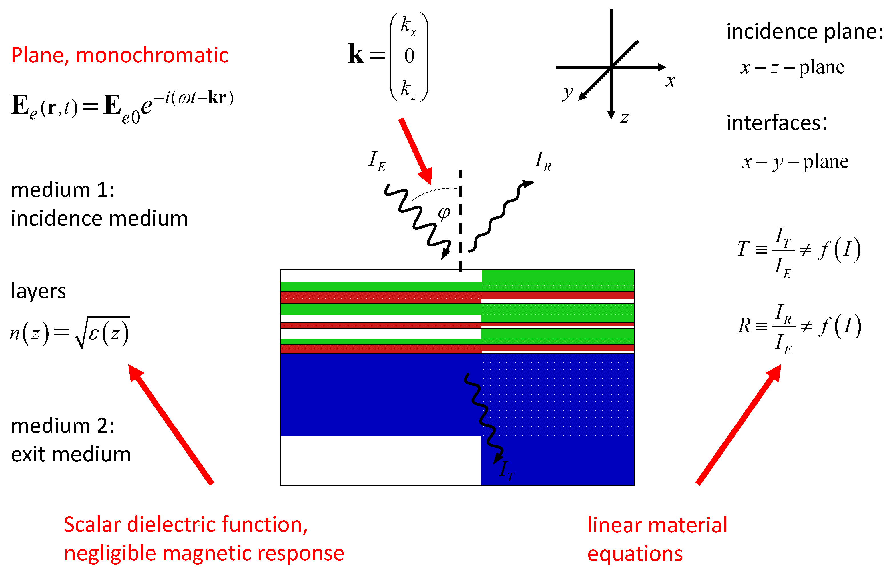
- We assume stratified media only. Consequently, the optical properties of the media shall depend on one coordinate (here, the z-coordinate, as seen in Figure 1) only. The optical parameters describing the materials may exhibit a discontinuous z-dependence, and in this case, the discontinuities in the optical parameters describe what we will further call interfaces. The interfaces are perpendicular to the z-axis.
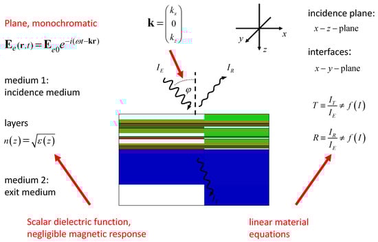 Figure 1. Illustration of the “standard model” of thin film optics. I is the light intensity; subscripts E, T, and R denote incident, transmitted, and reflected intensities. All other symbols are introduced in the next paragraph.
 - Consequently, the model system extends to infinity along the x- and y-axes.
- We further assume optical isotropy of all media. In addition, any magnetic response is neglected in our model.
- The semispace above the stratified medium is filled with a homogenous medium, called the incidence medium. As a postulate, light propagation in the incidence medium should be free of damping. On its bottom, the stratified medium faces a semispace filled with a further homogeneous medium, called the exit medium.
- It is assumed that a plane monochromatic electromagnetic wave is incident (from the incidence medium) on the stratified medium. In this case, an incident wavevector may be unambiguously defined. On this basis, an incidence angle may be introduced, which is zero for the particular case of normal incidence.
- At oblique light incidence, the wavevector of the incident wave and the z-axis allow the defining of an incidence plane.
- We further assume a three-wave scenario. That means that the incident wave gives rise to the generation of two other plane waves, propagating either in the exit medium (the transmitted wave) or in the incidence medium (the reflected wave).
- The materials are described in terms of linear optical constants only. As a consequence, reflectances and transmittances may be introduced that do not depend on the light intensity.
The set of requirements I–VIII defines what we will further call the standard model of thin film optics (see Figure 1). In many situations, the exit medium is associated with the substrate material. We further note that sometimes, the incidence medium is called the superstratum. Note that in this article, we will not explicitly consider the back side of the substrate (see [10,11]).
2.2. Material Description
2.2.1. Dispersion Models
When restricting on electric dipole interaction in optically isotropic materials (i.e., neglecting any magnetic response), the light–matter interaction results in the induction of a macroscopic polarization of the medium according to [10,12,13,14]:
Here, is the polarization of the medium, the vacuum permittivity, the electric field in the medium, and the real response function of the medium. is the time, and the integration variable stands for the time delay.
From the response function, the dielectric function (with —angular frequency of the incident light) of the medium is straightforwardly calculated according to the following:
Note that according to Equation (2), the dielectric function must depend on the light frequency (so-called dispersion) and is necessarily a complex quantity. For any real response function , from Equation (2) we immediately find the following:
In terms of the formulated model assumptions III and VIII, the optical constants n (the refractive index) and K (the extinction coefficient) are obtained from the complex dielectric function according to Equation (4):
2.2.2. Commonly Used Dispersion Models
There is a large amount of dispersion models used in the modern scientific literature, shown, for example, in [15,16,17,18,19,20,21,22,23,24,25]. Many of these models arise from making use of quantum mechanical features of the light–matter interaction, while in classical physics; there are basically three different dispersion models. We can only shortly present a selection of those models and start with the basic classical models:
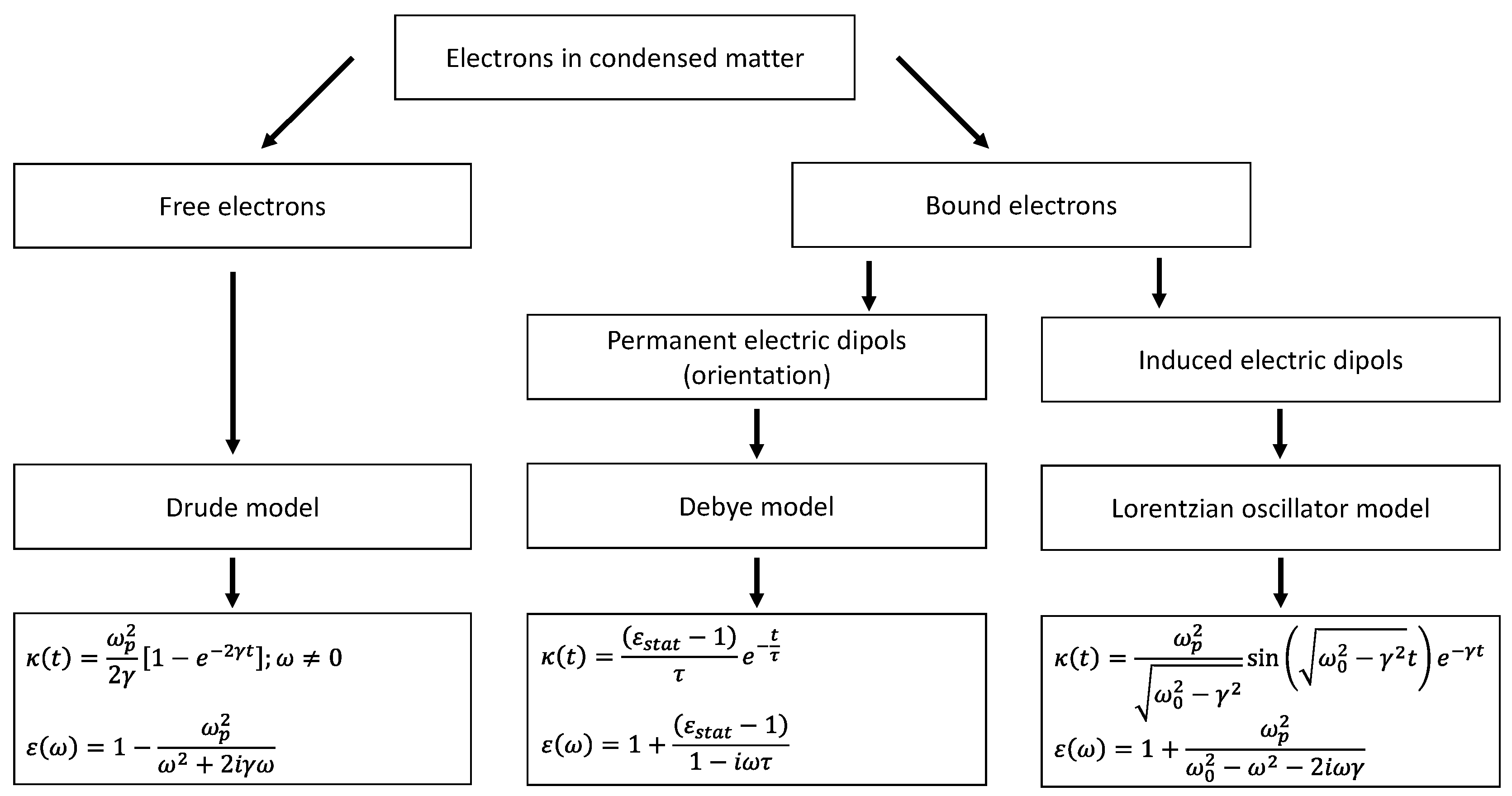
When classifying the electrons in a solid into free and bound electrons [26,27], three basic polarization mechanisms may be identified, which are presented in the following Scheme 1:

Scheme 1.
Basic polarization mechanisms in continous media.
Here, we have further introduced the resonance frequency , the damping constant , and the “plasma angular frequency” of the considered free or bound charge carriers (here, electrons), respectively. and are the charge and mass of the charge carriers, and stands for their concentration in the medium. The subscript “stat” denotes the static value of a given quantity.
Typically, none of the three mentioned models is applied in its pure form, because real matter has a tremendous number of degrees of freedom, all contributing to the full polarization of the medium under the action of an incident light wave. Therefore, the three basic models are usually properly superimposed to achieve a satisfying description of a realistic optical behavior. The multi-oscillator model is quite popular [27,28], but we will further focus on two special cases, namely the Brendel model [17] as well as the beta-distributed oscillator model (β_do model [18,19]).
Brendel model: It pursues the specifics of optical materials, which are characterized by fluctuations in the resonance frequencies within the material and thus provide an inhomogeneous line-broadening mechanism. When assuming a Gaussian distribution of angular resonance frequencies around a central frequency , an approximate calculation of the “averaged” dielectric function is performed by the equation
Here, is the standard deviation of the assumed Gaussian distribution, which defines the inhomogeneous contribution to the width of the absorption line defined by the imaginary part of ε. The shape of the absorption line is defined by the relation between and . In the case of , a Gaussian lineshape will be observed, while for , we will find a rather Lorentzian behavior. When both linewidth contributions are comparable to each other, we have , and then we obtain a so-called Voigt line.
The beta-distributed oscillator (β_do) model: In the β_do model, it is assumed that the envelope of the mentioned multiplicity of individual absorption lines is formed by a Beta-distribution given by
The real parameters , , , and are free parameters within the β_do model. The dielectric function is then given by the following:
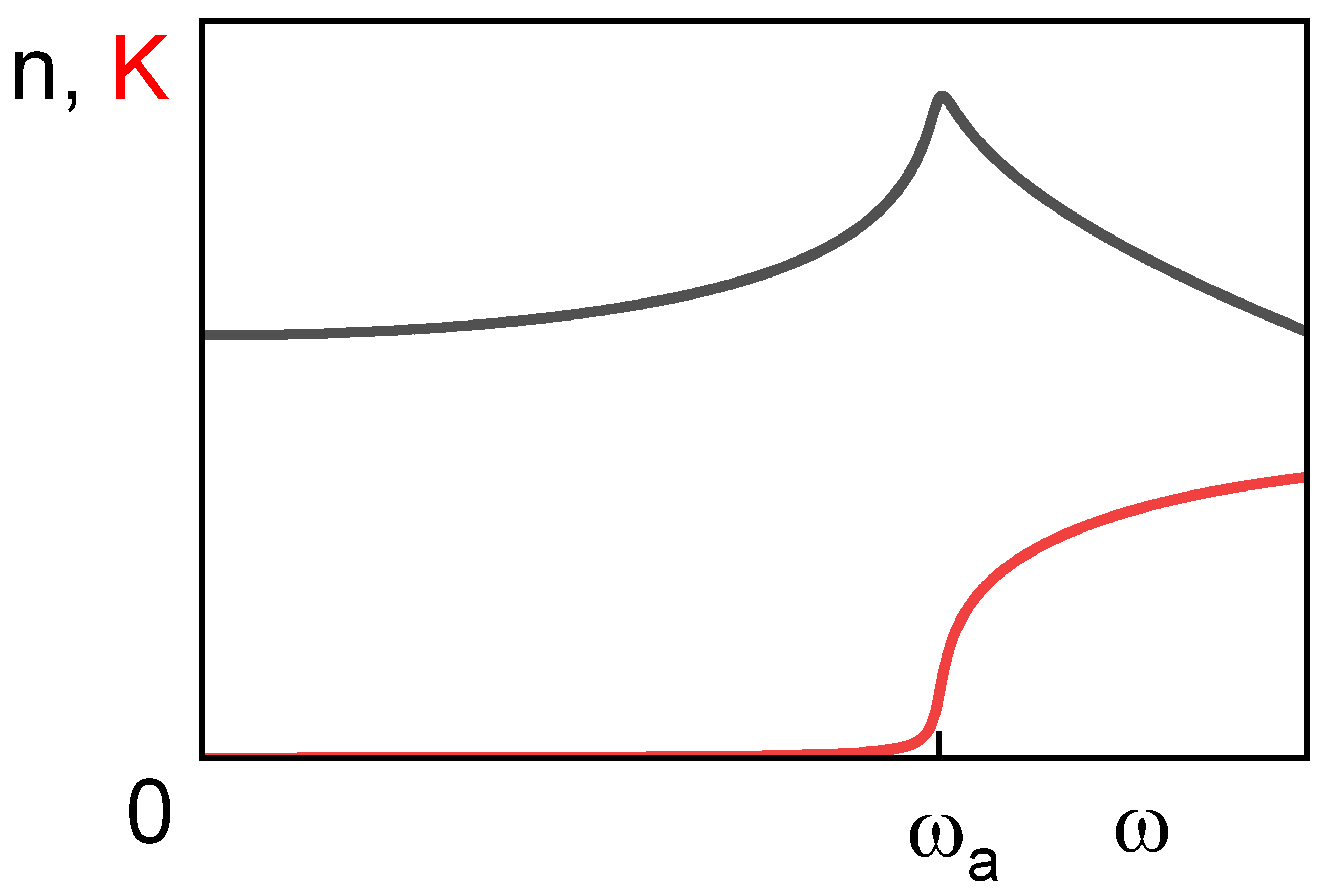
Here, is a further model parameter, which has the sense of an oscillator strength. Figure 2 shows an example on the optical constants’ dispersion as described in terms of the β_do model. The total of six free parameters provides some flexibility in modeling various (in particular asymmetric) absorption features, in particular in modeling what is called an absorption edge, defined by the parameter (or threshold frequency or absorption onset frequency) in Equation (6).
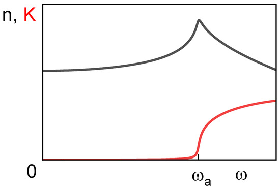
Figure 2.
Optical constants as modeled by the β_do model. The indicated value marks the absorption edge.
As already mentioned, there is a tremendous amount of further dispersion models, particularly accounting for the quantum mechanical nature of light–matter interaction [13,14,15,20,21,22,23,24,25,29,30,31,32,33,34,35]. We will shortly mention the Tauc–Lorentz, Cody–Lorentz, as well as the Forouhi–Bloomer models, because of their ability to model the threshold character of light absorption in dielectric or semiconductor coatings by introducing an absorption edge.
In the Tauc–Lorentz model, the imaginary part of the dielectric function of a single oscillator model is merged together with the Tauc edge [30,31,32] to generate the imaginary part of the dielectric function of the Tauc–Lorentz model according to [20,21], leading to Equation (8):
Here, is the absorption edge described in terms of the Tauc optical gap. Compared to the usual writing, Equation (8) is generalized to negative frequency arguments in order to comply with Equation (3). The corresponding real part is calculated in terms of a Kramers–Kronig relation (see later point Section 2.2.3). Explicit expressions can be found, for example, in [20,33].
The introduction of the Tauc gap in amorphous semiconductor optics is connected to the assumption of a constant (frequency-independent) transition matrix element of the momentum operator. If, on the contrary, constancy of the electric dipole moment operator is presumed, one arrives at the Cody description of light absorption in the vicinity of the absorption gap, which results in the definition of the Cody gap [35]. With corresponding modifications in Equation (8), the Cody–Lorentz model may be formulated [22]. To our knowledge, the Tauc–Lorentz model is more frequently used in practice than its counterpart, the Cody–Lorentz relation.
In the Forouhi–Bloomer model (we restrict here on the version for amorphous solids [23]), explicit expressions for n and K are derived according to the following:
The -, -, and -values are constants. For uniformity reasons, Equation (9) is written here in terms of the angular frequency, which is in contrast to the original publication where the photon energy was used. What appears rather strange is the asymptotic behavior for . This has been recognized early and gave rise to corresponding criticism [20]. Nevertheless, the model is frequently applied to spectra analysis in the vicinity of the fundamental absorption edge.
2.2.3. Kramers–Kronig Consistency
Any physically reasonable dielectric function must suffice the Kramers–Kronig relations [10,12,13]:
With VP—Cauchys principal value of the improper integral, and —integration variable. The term in Equation (11) arises from the singularity in the Drude function at and is only relevant in electric conductors with a static electric conductivity . The Drude, Debye, and oscillator models are consistent with Equations (10) and (11), and so are their linear superpositions. As a special case, the β_do model is Kramers–Kronig consistent as well. The situation is a bit more complicated with the Brendel model [36] because the dielectric function according to Equation (5) contains a contribution with a vanishing resonance frequency, which becomes equivalent to a Drude-like term and therefore requires an addendum to Equation (11) similar to what we have in the case of conductors. The problem may be overcome when using an appropriately apodised Gaussian function in Equation (5) instead.
The Campi–Coriasso model [37,38] seems to be the first Kramers–Kronig consistent model combining the oscillator model with Tauc’s law [39]. It uses the same number of parameters with the same meaning as the Tauc–Lorentz model, but its parametrization is different and it is far less common. In the original work, no analytical expression for the real part of the dielectric function is provided but can be found in [39], where a good overview on models combining Tauc’s law and the Lorentz model is also given. The author of [39] concludes on the Kramers–Kronig consistency of both the Tauc–Lorentz and Cody–Lorentz approaches, while the Forouhi–Bloomer model is claimed as Kramers–Kronig inconsistent.
In [40], a different physically consistent model combining the oscillator model with Tauc’s law is presented. It is called Advanced Dispersion Model and is a precursor of the Universal Dispersion Model [24]. In contrast to the latter, it requires a priori information about the physical and chemical structures of the films since the model contains physical parameters specific for the material, such as atomic fractions.
In concluding this paragraph, let us mention that the Kramers–Kronig relations represent a rather general quantitative formulation of the physical connection between light refraction and absorption phenomena. In fact, those connections are intuitively used by any coating practitioner. It is well known from coating practice that materials with a large refractive index tend to have smaller optical gaps than materials with a smaller refractive index. These correlations are formulated in semi-empirical rules like the Moss and Ravindra rules [41], and represent a useful guide in any realistic coating design procedure.
3. Model Violations
3.1. General
In this article, we will separately deal with model violations concerning geometrical features of our “standard model”, and those concerning modeling the optical material constants. Concerning geometry, it is clear that the idealized model requirements I–VIII, as formulated in Section 2.1, will never be fulfilled in practice, and therefore, model violations are unavoidable in practice. Therefore, we will discuss prominent examples, effects, and their possible application potential. To a certain extent, this also concerns modeling of materials, because no real material is absolutely homogeneous, isotropic, electrically insulating, and so on. What we will not discuss here are specific effects arising from the use of Kramers–Kronig inconsistent dispersion models in practical modeling of the coating optical response in broad spectral regions. We see no real necessity to make use of inconsistent models, because there are enough Kramers–Kronig consistent dispersion models available, and it is hard to recognize the generation of new application ideas from the use of physically inconsistent models.
3.2. Geometry
3.2.1. Restricted Beam Dimensions
We return to our standard model (Figure 1) and turn to the discussion of selected model assumption violations. Within this section, we shortly discuss a phenomenon called the Goos–Hänchen shift [42] for historical reasons.
In this context we consider a situation, that in contrast to model assumption V, the illumination area is spatially restricted. In particular, we assume some kind of illumination slit that is elongated along the y-axis while being spatially restricted along the x-axis (Figure 3).
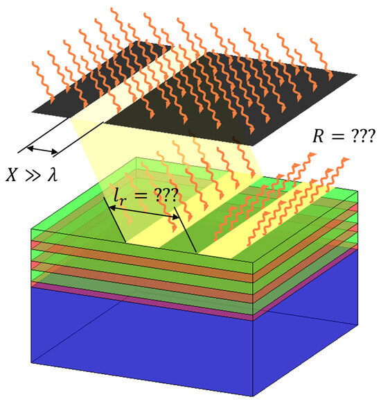
Figure 3.
Violation of model assumption V, resulting in a lateral shift (exaggerated for visibility) of the reflected light beam.
Clearly, even in this modified illumination geometry, the incident light beam may be reflected or transmitted at the sample surface. Once we have a spatially restricted illumination spot, it makes sense to ask where the light leaves the sample.
Historically, this was first investigated in internal total reflection conditions at a single interface. As a matter of fact, the totally reflected light beam turns out to be laterally shifted along the x-axis with respect to the incident light beam for a characteristic distance lr. This is the so-called Goos–Hänchen shift [42,43]. It turned out later that this phenomenon is however not restricted to surfaces in total internal reflection conditions. In optical coatings, lateral shifts up to the sub-millimeter range have been experimentally established [44].
In [43], Kurt Artmann was able to show that the value of the Goos–Hänchen shift depends on the first derivative of the phase of the complex reflection coefficient with respect to the incidence angle . The idea behind his model is that the spatially restricted illumination area is equivalent to relaxing the model requirement V. Hence, he assumed a certain distribution of incident plane waves with different incidence angles, and the lateral shift is then obtained as follows:
Here, denotes the refractive index of the incidence medium.
Again, the effect is not only relevant in total internal reflection conditions [10]. It has been found in the vicinity of the Brewsters angle with p-polarized light [45], at interfaces between transparent and absorbing media [45,46,47,48,49], as well as at metal surfaces [48,49].
Artmann’s argumentation is general enough to be applicable to thin film stacks as well [44,50]. Correspondingly, lateral shifts in transmission () and reflection () are estimated in terms of Equation (13):
The lateral shift according to Equation (13) depends on the wavelength of the incident light. Potential applications therefore pursue wavelength demultiplexing tasks [51,52].
3.2.2. Polarization Leakage
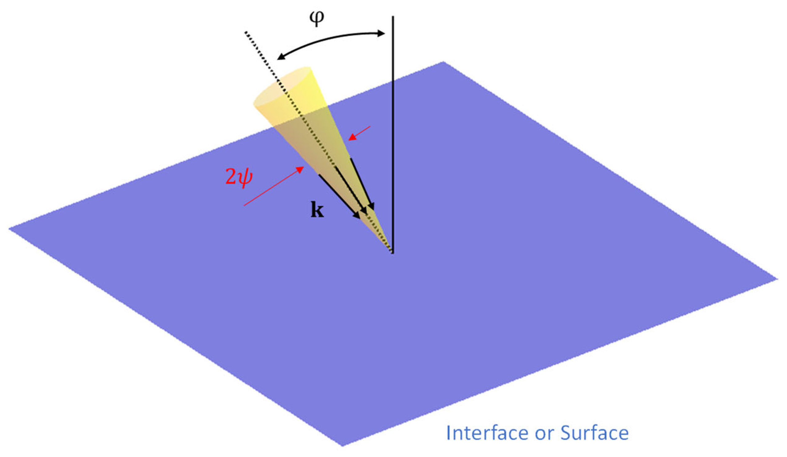
In this section, we discuss the consequences of a violation of model requirement VI (no unambiguously defined incidence plane). Let us imagine a situation where the assumed plane sample surface is illuminated by light consisting of many different rays with different individual wavevectors. Let us further restrict on a simple model case, where all incident wavevectors are confined in a cone characterized by an apex-semiangle (Figure 4) [53]. The angle now denotes the angle between the surface normal and the symmetry axis of the cone (Figure 4, dotted line). The described situation may correspond to an oblique incidence of focused or defocused light.
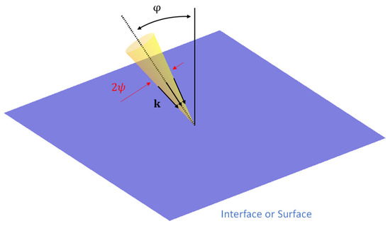
Figure 4.
Assumed illumination geometry resulting in polarization leakage.
However, because of the assumed conical light incidence geometry, it is now no more possible to define an incidence plane in the strong sense. Indeed, each of the light rays that form the cone defines an individual incidence plane, and consequently, the termini of s- and p-polarization [10] use their assumed strong sense. Indeed, for example, light that is s-polarized with respect to the nominal incidence plane defined by the symmetry axis of the cone is not necessarily s-polarized for the individual incidence planes relevant for other k-vectors; instead, it may contain p-polarized components. The result is an effect called polarization leakage. It is rather disturbing in any real experiment performed with linearly polarized light and, in particular, destroys the performance of thin film light polarizers.
Quantitatively, the polarization leakage may be introduced in the following manner. Let the nominal incidence plane (as formed by the symmetry axis of the cone and the surface normal) coincide with the x-z-plane. Moreover, let the incident light be linearly polarized with the -vector parallel to the y-axis. Hence, with respect to the nominal incidence plane, the light should be s-polarized. However, because of the spread in directions of the individual k-vectors, this is not true for all light rays. Therefore, the transmittance relevant for light polarized along the y-direction () appears to be a biased superposition of the s-polarized contribution () and the p-polarized contribution (). Hence, we define through the following:
For a vanishing polarization leakage, i.e., , the transmittance of y-polarized light naturally coincides with that of s-polarized light. Obviously, the polarization leakage will increase when increases. For other polarizations of the incident light, may be introduced in an analogous manner.
While a general theory of the polarization leakage is developed in [54], a somewhat simpler but less general treatment restricted to a Lambertian intensity distribution results in the manageable expression Equation (15) (see [53]):
In deriving Equation (15), is assumed.
Note that the leakage is determined by the illumination geometry only, the apex- semiangle is given in radians. Therefore, improvements of the coating design have no effect on the polarization leakage.
As it turns out from Equation (15), the polarization leakage may be reduced by enlarging the angle . In practice, that gave rise for the development of completely new types of thin film polarizers, working at incidence angles substantially larger than the usually applied incidence at 45° [55]. The working principle of these polarizers is based on attenuated total internal reflection at certain internal interfaces, and thus represents an example of the development of completely new optical components stimulated by the emergence of an originally disturbing effect like the polarization leakage.
3.2.3. Rough Surfaces
Rough surfaces, as well as any laterally structured coatings, violate the model assumption I defined in Section 2.1 because they introduce an additional - and/or -dependence of the dielectric function. Indeed, any surface profile is usually defined in terms of a surface height function . The rms surface roughness is then defined through the following:
where is a characteristic length scale. Usually, in a practical situation, the surface profile is not exactly known. Let us for simplicity consider the situation of a one-dimensional surface height profile that is assumed to be known on a certain length interval in a number of points. That interval may then periodically continue, so that it can be approximated by the following [56]:
In this case, the rms surface roughness can be written as follows:
From here, we obtain the expressions for the so-called small-scale roughness and large-scale roughness via the following:
Small- and large-scale roughnesses have a different impact on the optical properties of a coating. Large-scale roughness gives rise to diffuse light scattering and thus provides an optical loss mechanism. Small-scale roughness, on the contrary, rather acts like an antireflection coating. A small-scale roughness is usually modeled by introducing a fictive mixture layer on the surface, making use of a mixing model like the Lorentz–Lorenz or the Maxwell Garnett approach. This calculation strategy is well established and incorporated today in commercially available film characterization software, particularly for ellipsometry purposes [57]. The introduction of an (optically homogeneous) mixture model eliminates the x- and y-dependence of the optical properties from the system, so that the calculation of the optical properties may again be performed in terms of the model assumptions formulated in Section 2.1.
The situation is different in the case of a large-scale roughness. Different approximation formulas have been proposed to incorporate the scatter losses into the optical model. A crucial point is that the effect of the roughness on the thin film spectra is now twofold: The surface roughness may not only change the propagation direction of the incident light through elastic scatter, but has also an impact on the coherence of light trains superimposing as a result of multiple internal reflections at the interfaces of the film system. Therefore, at the moment, no unique generally accepted manageable approach is available, but there exists a large diversity of different approaches (as examples, we cite [56,58,59,60,61,62,63,64,65,66,67,68,69,70,71,72,73,74,75,76,77,78,79,80,81,82,83,84,85,86,87,88,89,90,91]), all having their individual strength and shortcomings. As seen from the references, surface roughness in optical coatings is a hot topic from the sixtieth of the last century of the previous millennium until today.
A detailed discussion of the available literature is beyond the frames of this review. Clearly, a rigorous electrodynamic treatment of wave propagation through a system with a specified surface geometry will provide the necessary information, but in thin film practice, any practitioner will seek for a couple of manageable formulas that allow for a quick-and-dirty estimation of the effect of roughness on a spectrum that is otherwise calculated in the usual way. We therefore limit the discussion of large-scale roughness to the presentation of a set of estimation formulas, that have proven useful for estimating the roughness-induced changes in specular reflectance and transmittance at interfaces compared to the ideally flat surface model (Table 1). Thereby, the model for large-scale roughness by A. V. Tikhonravov [56] is limited to normal light incidence and non-absorbing materials only. It can be extended to the case of oblique light incidence, as exemplified in [58,79]. Table 1 summarizes several proposed versions of scatter factors S relevant for reflection (r) and transmission (t). In the calculations, these scatter factors appear as prefactors to the usual Fresnel field transmission and reflection coefficients.

Table 1.
Overview on scatter factors and applied in various references. j is the layer number in a stack, the vacuum wavelength, and the effective refractive index and , .
3.2.4. Coherence
In thin film optics, a loss in coherence between multiply internally reflected waves is usually caused by either a coating thickness that increases the coherence length of the incident light, or by the loss of phase information of the wave when passing rough interfaces (see Section 3.2.3.). In this section, our focus will be on the first mechanism.
In optical multilayer systems with smooth interfaces, a distinction is usually made in the description between the extreme cases of incoherent (e.g., substrate with consideration of the back side) and coherent light propagation [11]. In the case of incoherent light propagation, no phase information is included, because the coherence length of the light is assumed to be smaller than the layer thickness. Therefore, no interference effects occur and only the wave amplitudes are relevant and geometrical optics can be used for modeling.
In the case of coherent light propagation, the coherence length is assumed to be significantly larger than the layer thickness. For this reason, the phase information remains important and interference effects between multiply reflected waves will occur. Therefore, the wave optic is the corresponding theoretical model here.
Optical coatings containing both types of layers can be modeled with the general transfer matrix method outlined in many textbooks (e.g., [92]). In the case of anisotropic layers, a generalized method is proposed in [93].
In the intermediate regime, when the layer thickness is in the range of the coherence length, the two mentioned extreme cases are of no relevance, and an adapted theoretical approach based on partial coherence is required.
Bearing in mind that the coherence length is affected by spectral resolution and wavelength of the light source, a given sample may appear either “coherent” or “incoherent”, depending on the illumination conditions [10]. When an optical coating is measured in a sufficiently broad spectral range, the transition from “coherent” to “incoherent” may even be observed within a single transmission or reflection spectrum. As a result, the loss in coherence may be observed by a depletion of the amplitude of the interference fringes usually observed in both transmission and reflection spectra.
Let us finish this section with a short literature review. Initially, the theoretical description of partial coherence was limited to single-layer coatings at normal incidence [94], but later these limitations could be eliminated in a more general theory [95]. In this approach, a complex degree of coherence (cdc) has been introduced. The limiting cases of the absolute values are |cdc| = 0 for incoherent and |cdc| = 1 for coherent light propagation. In [77], a simpler coherence function is proposed and spectral averaging over an interval is used.
In [96], partially coherent light propagation is also modeled with the transfer matrix method, but the transition from coherent to incoherent propagation is achieved by introducing a random phase of increasing intensity. In [97], the coherence length is considered using a Fourier transform of a randomly generated partially coherent wave. Thereby, the statistical field distribution of partially coherent light is modeled using a rigorous coupled wave analysis.
In [72,75], a generalized matrix method is presented, where interface roughness has been addressed as a special case of partially coherent light propagation. The phase-shift integration method in [98] provides an alternative mathematical approach for the modeling and is used to derive an analytical expression for irradiance at an arbitrary depth of the multilayer stack. The method is advantageous for gradient optimization methods because analytical layer thickness derivatives are provided.
In [99], the net-radiation method is adapted for modeling the reflectance, transmittance, and absorption depth profile of thin film multilayer structures such as solar cells. Thereby, an arbitrary multilayer structure with coherent, partly coherent, and incoherent layers can be simulated more accurately at much lower computational cost.
A generalized transmission line method (TLM) is outlined in [100] and applied to thickness determination of individual layers of an organic light-emitting diode. Additionally, the approach is used for calculation of the external quantum efficiency of an organic photovoltaic with partially coherent rough interfaces between the layers.
3.3. Materials
3.3.1. Optically Anisotropic Materials
In fact, optical material anisotropy and its relation to optical thin film theory and practice is well understood and documented in the realm of (variable angle) spectroscopic ellipsometry [101,102,103]. Software packages for ellipsometry data analysis therefore usually allow modeling certain types of optical anisotropy [104,105]. Therefore, there is no principal difficulty in generalizing the thin film model to anisotropic materials. We mention that anisotropic film materials allow designing and manufacturing of novel superior polarizing components, as already demonstrated in the field of Giant Birefringent Optics (GBO [106,107]).
3.3.2. Spatial Dispersion
The introduction of the dielectric function according to Equations (1) and (2) does not consider effects caused by non-locality of the dielectric response [12]. Indeed, it may happen that the polarization in a given point in space depends on the electric field in that point, and additionally on the field in surrounding points (non-local response). Then, instead of Equation (1), we should write the following:
The response function is now time- and coordinate-dependent. denotes the volume where is essentially different from zero.
Non-locality has a striking effect on the dielectric function. It is now defined as follows:
The k-dependence of is called spatial dispersion. As a rule of thumb, one may note that the usual dispersion becomes significant when the oscillation period of the light becomes comparable with characteristic times describing the dynamics of the medium (resonance phenomena). Spatial dispersion, on the contrary, becomes significant when the wavelength of the light becomes comparable with characteristic spatial dimensions in the medium. Usually, when performing spectroscopy in the visible and adjacent spectral regions, spatial dispersion may therefore be neglected.
However, there are exclusions from this rule. In metal island films, spatial dispersion may matter [108,109]. Also, as pointed out already in [12], non-local response effects may impair the practical relevance of the Kramers–Kronig relations Equations (10) and (11), particularly in metals. Generally, an increase in the refractive index near a resonance will decrease the wavelength of the propagating light, which may also give rise to effects of spatial dispersion. In particular, it may give rise to optical anisotropy in an otherwise isotropic material (compare Section 3.3.1). Note, in this context, that non-locality is naturally included in the quantum mechanical expression for the dielectric function in semiconductor theory [110,111].
3.3.3. Time-Dependent Material Properties
The corresponding basics have already been developed in the 50th of the previous century [112,113]. Instead of Equations (1) and (2), we now have the following:
This way, we have introduced what may be called a “time-dependent dielectric function”, while relaxing the natural requirement of time homogeneity.
Let us, in a short manner, note some specifics of wave propagation in the presence of time inhomogeneity [114]. It is well known that spatial inhomogeneity preserves the light frequency but changes the wavelength. Time inhomogeneity, on the contrary, changes the light frequency while preserving the wavelength. This is a direct conclusion from Noethers theorems [10,115,116].
A temporal interface is defined as a discontinuity in , while a spatial (i.e., usual) interface results from a discontinuity in . Both kinds of interface result in the generation of a backtraveling (reflected) wave when an incident wave arrives at the interface. However, at a temporal interface, the sum of transmittance and reflectance may exceed 1, which is in contrast to the situation at a spatial interface between two passive media [113,114].
The combination of several temporal interfaces allows constructing temporal coatings [117]. Even more futuristic, the combination of temporal and spatial interfaces in an optical component leads us to the concept of a time-varying metamaterial [118].
3.3.4. Non-Linear Response
According to model assumption VIII, T and R are independent of the incident light intensity. However, T and R may become intensity-dependent, provided that Equation (1) is replaced by its non-linear counterpart according to [119]:
In the more familiar frequency domain, Equation (24) may be written in the following simplified manner:
As is evident from Equation (24) or Equation (25), non-linear optical effects become significant only at rather large light intensities. Relevant with respect to thin film optics examples include harmonic generation as well as the observation of intensity-dependent transmittances or reflectances [120,121,122,123,124]. In ultrashort light pulses, peak intensities may become rather large [125]. In such a constellation, the reflectance of a thin film reflector may be significantly reduced when compared to what is expected from the standard (linear) theory. The physical process behind this is called non-linear absorption. Let us mention for completeness that the second harmonic generation is related to second-order terms in Equations (24) and (25), while the third harmonic generation as well as non-linear absorption result from the third-order terms.
As an example, Figure 5 shows the simulated normal incidence reflectances and transmittances of three fictive antireflection coatings depending on the intensity of the incident light. For details of the simulation algorithm, see [126,127,128], but let us shortly mention that the calculation of T and R is based on the solution of a system of equations:
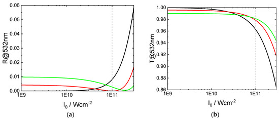
Figure 5.
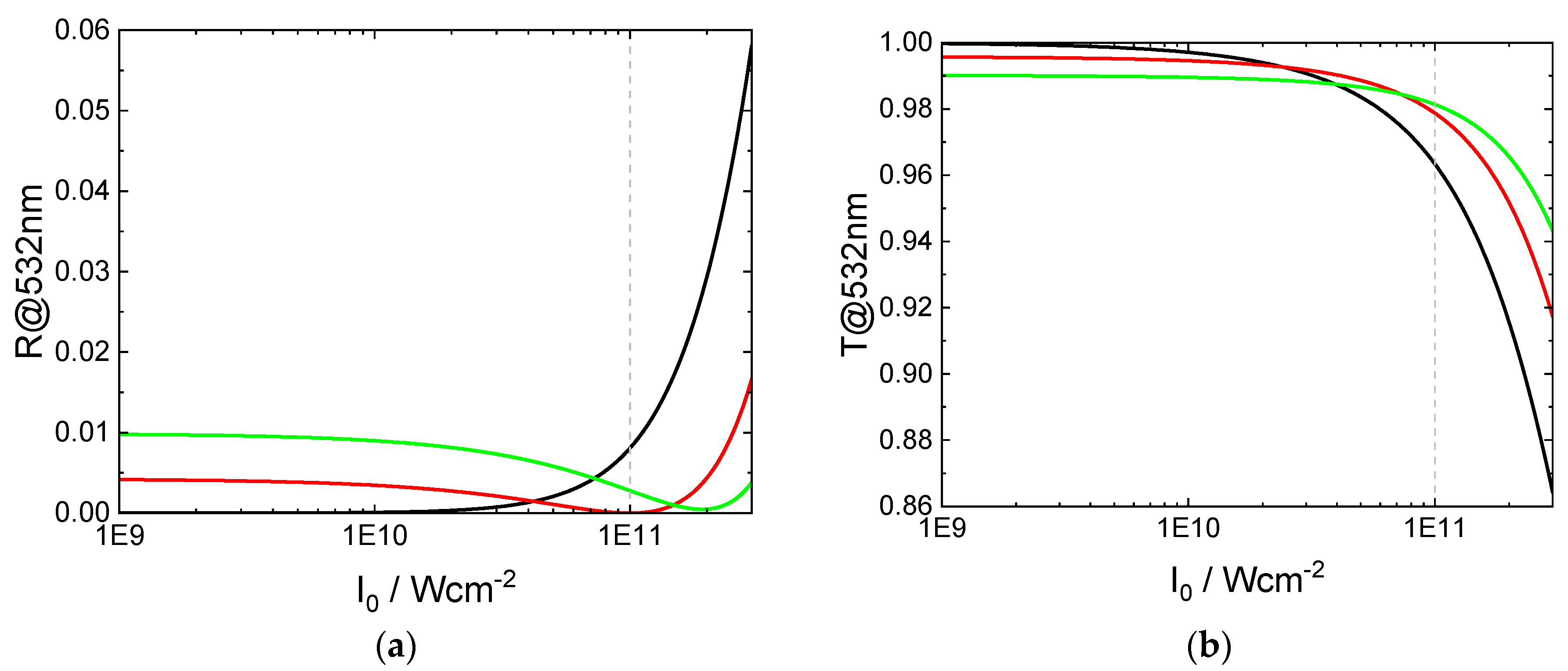
Comparison of (a) reflectance R and (b) transmittance T (normal incidence) of the antireflection designs specified in Table 2 as a function of the incident light intensity. For more details, see text.
Here, for simplicity, normal incidence is assumed. stands for the electric, and for the magnetic field strength. This is a non-linear system of equations which needs to be solved numerically for the assumed z-dependence of and . Note that in the special case of , Equation (26) becomes linear and coincides with the system of equations relevant for calculating the linear response of any stratified medium (compare [9,10,26]). In particular, the well-known matrix formalism may be directly derived from the linear version of Equation (23).
After having solved Equation (26) with proper boundary conditions, the electric field transmission and reflection coefficients (Fresnel coefficients and ) are obtained from the following:
Here, air is assumed as incidence medium. The interface between air and the stratified medium is at .
Assuming now , all materials are characterized by four optical constants. Indeed, in addition to the linear optical constants and , the real as well as the imaginary parts of have to be taken into consideration. As a result, the calculated transmittance and reflectance turn out to be intensity-dependent.
Let us finish this small section with a model calculation (see Figure 5). We start from a simple V-coating [7,8] that might be in use as antireflection coating at a wavelength of 532 nm (black line). In addition, the red line in Figure 5 shows the performance of a modified V-coating optimized for smallest reflectance at an incident intensity of 1011 Wcm−2 taking non-linear susceptibilities into account, while the green line corresponds to the performance of a design optimized for highest transmittance at 1011 Wcm−2. Basic design parameters are summarized in Table 2.
Table 2.
Basic input parameters for the calculations provided in Figure 5. Substrate is fused silica (), ambient air, normal incidence. Layer 1 is next to substrate, layer 2 next to ambient.
Obviously, at low light intensities, the traditional V-coating is best in antireflection performance. However, the picture changes at larger light intensities. Therefore, in non-linear optics, new optical coating design solutions may have to be developed.
Thus, in non-linear optics, optical coating design tasks are of increased complexity when comparing with the linear case. Particularly, we mention the increased number of optical material parameters that need to be known and considered in the design calculation.
The intensity dependence of the optical performance of the coating is a direct consequence. A design that is optimized for a certain light intensity is not necessarily a good choice for application at other intensities (compare Figure 5).
Compared to the linear task, the determination of non-linear optical parameters needs much more complex and expansive equipment, as well as a considerable larger measurement effort [129]. We note that it might be prospective to make use of parametrized dispersion laws for non-linear optical constants [130], calibrated by a restricted set of experimental data. We also mention that there exists a couple of estimation formulas for realistic non-linear refractive indices [131,132,133], based on the generalized Millers rule [134].
3.3.5. Thickness-Dependent Optical Constants
The basic concept of optical thin film theory described so far relies on the possibility to perform a clear separation between material parameters (optical constants) and geometrical parameters (thicknesses) from each other [16]. This is a fundamental requirement, and it allows, for example, in a coating design task, the combining of optical constants and film thicknesses in an arbitrary manner. In fact, this is not always possible. Once the optical constants represent macroscopic parameters, obtained after averaging the atomic or molecular responses in a thermodynamically relevant volume fraction, this concept may collapse when the film thickness becomes too small. Thus, atomic or molecular monolayers are more reliably modeled in terms of the microscopic polarizability [135,136]. This is clearly an extreme example, but a “thickness dependence” of optical constants is also obtained in thin metal films, when the thickness becomes smaller than the mean free path of the conduction electrons in the metal [137,138,139]. Also, a clear separation between effective optical constants and thickness of a metal island film is problematic [140]. In a more recent publication, Willey [141] proposed a design procedure for metal-island-film-based coatings while taking the thickness dependence of their effective optical constants into account explicitly.
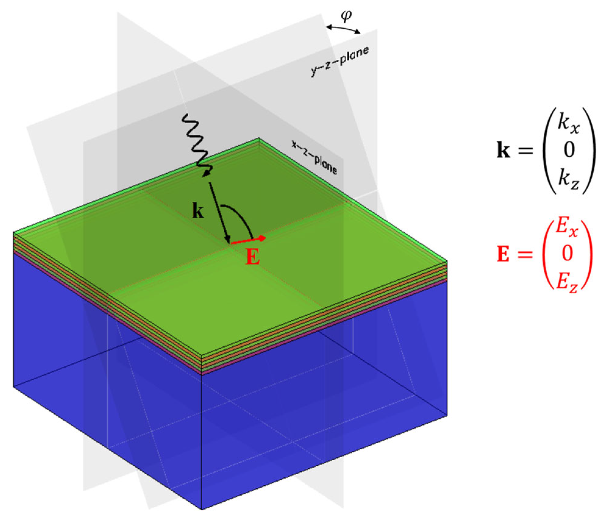
Presently, research is also directed on making use of nanolaminates as versatile building blocks in optical coating design [142,143,144,145,146]. The hope is that because of quantum confinement effects [147,148], new combinations of optical gap and refractive index may become accessible, thus overcoming the restrictions emerging from the Moss or Ravindra rules [41]. However, those nanolaminates are strongly anisotropic (see Figure 6 and Figure 7), and the efficient exploitation of confinement effects may be restricted to special illumination and polarization geometries. Thus, in the case of normal incidence (Figure 6), the electric field strength vector is in the x-y-plane and cannot induce electric dipole transitions along the z-axis (i.e., between different discrete energy levels of the electron moving along the confinement direction in the quantum well; see the selection rules discussed in [148]). At oblique incidence and p-polarization, however, such transitions shall be possible, because the electric field strength vector has a non-vanishing component along the z-axis. Hence, even the absorption behavior of such nanolaminates is expected to be strongly anisotropic, which offers new development directions in the field of polarizing absorptive optics.
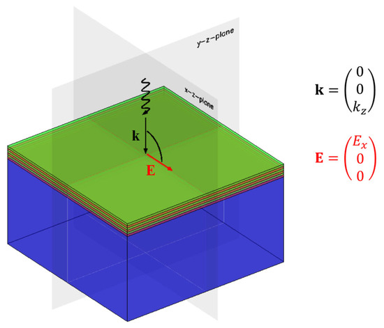
Figure 6.
Nanolaminate at normal light incidence.

Figure 7.
Nanolaminate at oblique light incidence and for p-polarization.
4. Summary and Challenges
We have reviewed important facets of the typical thin film optical model. According to our primary intention, idealized model assumptions have first been formulated, and then opposed to real geometry and measurement conditions that give rise to model assumption violations in practice. We emphasize that knowledge of these possible model violations and their effects is important for at least three reasons.
- i.
- They enable the user of commercial optical film calculation software to critically evaluate the practical value of a calculation result.
- ii.
- They enable the practitioner to understand the reason for discrepancies between the promised and measured performance of purchased thin film optical components.
- iii.
- They define important topics for the design of university courses on applied thin film spectroscopy.
In addition to this, we tried to demonstrate that the effects caused by certain model violations had a stimulating impact on the development of novel optical components. Examples are provided by new demultiplexing devices, Giant Birefringent Optics, as well as new thin film polarizer, dielectric reflector, antireflection coating, and absorber coating designs.
Author Contributions
Conceptualization, O.S.; methodology O.S. and S.W.; software S.W.; writing—original draft preparation, O.S.; writing—review and editing, O.S. and S.W.; All authors have read and agreed to the published version of the manuscript.
Funding
This research was funded by Fraunhofer Society, grant number 510076.
Data Availability Statement
No data available.
Conflicts of Interest
The authors declare no conflicts of interest.
References
- Film Wizard. Available online: https://sci-soft.com/product/film-wizard (accessed on 18 December 2024).
- FilmStar. Available online: https://ftgsoftware.com (accessed on 18 December 2024).
- Essential Macleod. Available online: https://www.thinfilmcenter.com/essential.php (accessed on 18 December 2024).
- OptiLayer. Available online: https://optilayer.com (accessed on 18 December 2024).
- OTF Studio. Available online: https://otfstudio.com (accessed on 18 December 2024).
- Tikhonravov, A.V. Some theoretical aspects of thin-film optics and their applications. Appl. Opt. 1993, 32, 5417–5426. [Google Scholar] [CrossRef] [PubMed]
- Thelen, A. Design of Optical Interference Coatings; McGraw-Hill Book Company: New York, NY, USA, 1989. [Google Scholar]
- Macleod, H.A. Thin-Film Optical Filters; Adam Hilger Ltd.: Bristol, UK, 1986. [Google Scholar]
- Furman, S.A.; Tikhonravov, A.V. Basics of Optics of Multilayer Systems; Edition Frontieres: Gif-sur-Yvette, France, 1992. [Google Scholar]
- Stenzel, O. The Physics of Thin Film Optical Spectra: An Introduction, 3rd ed.; Springer: Berlin/Heidelberg, Germany, 2024. [Google Scholar]
- Harbecke, B. Coherent and incoherent reflection and transmission of multilayer structures. Appl. Phys. B 1986, 39, 165–170. [Google Scholar] [CrossRef]
- Landau, D.; Lifshitz, E.M. Electrodynamics of Continuous Media; Volume 8 of A Course of Theoretical Physics; Pergamon Press: Oxford, UK, 1960. [Google Scholar]
- Yu, P.Y.; Cardona, M. Fundamentals of Semiconductors: Physics and Material Properties, 4th ed.; Springer: Berlin/Heidelberg, Germany, 2010. [Google Scholar]
- Gross, R.; Marx, A. Festkörperphysik; Walter de Gruyter GmbH: Berlin, Germany; Boston, MA, USA, 2014. [Google Scholar]
- Kittel, C. Introduction to Solid State Physics; John Wiley and Sons, Inc.: New York, NY, USA; London, UK; Sydney, Australia; Toronto, ON, Canada, 1971. [Google Scholar]
- Stenzel, O. Optical Coatings: Material Aspects in Theory and Practice; Springer: Berlin/Heidelberg, Germany, 2014. [Google Scholar]
- Brendel, R.; Bormann, D. An infrared dielectric function model for amorphous solids. J. Appl. Phys. 1992, 71, 1–6. [Google Scholar] [CrossRef]
- Wilbrandt, S.; Stenzel, O. Empirical extension to the multioscillator model: The beta-distributed oscillator model. Appl. Opt. 2017, 56, 9892–9899. [Google Scholar] [CrossRef]
- Stenzel, O.; Wilbrandt, S. Beta-distributed oscillator model as an empirical extension to the Lorentzian oscillator model: Physical interpretation of the β_do model parameters. Appl. Opt. 2019, 58, 9318–9325. [Google Scholar] [CrossRef]
- Jellison, G.E.; Modine, F.A. Parameterization of the optical functions of amorphous materials in the interband region. Appl. Phys. Lett. 1996, 69, 371–373. [Google Scholar] [CrossRef]
- Jellison, G.E. Spectroscopic ellipsometry data analysis: Measured versus calculated quantities. Thin Solid Films 1998, 313–314, 33–39. [Google Scholar] [CrossRef]
- Ferlauto, A.; Ferreira, G.; Pearce, J.M.; Wronski, C.; Collins, R.; Deng, X.; Ganguly, G. Analytical model for the optical functions of amorphous semiconductors from the near-infrared to ultraviolet: Applications in thin film photovoltaics. J. Appl. Phys. 2002, 92, 2424–2436. [Google Scholar] [CrossRef]
- Forouhi, R.A.; Bloomer, I. Optical dispersion relations for amorphous semiconductors and amorphous dielectrics. Phys. Rev. B Condens. Matter 1986, 34, 7018–7026. [Google Scholar] [CrossRef]
- Franta, D.; Nečas, D.; Ohlídal, I. Universal dispersion model for characterization of optical thin films over a wide spectral range: Application to hafnia. Appl. Opt. 2015, 54, 9108–9119. [Google Scholar] [CrossRef]
- Franta, D.; Vohánka, J.; Čermák, M. Universal Dispersion Model for Characterization of Thin Films Over Wide Spectral Range. In Optical Characterization of Thin Solid Films; Stenzel, O., Ohlídal, M., Eds.; Springer Series in Surface Sciences; Springer: Cham, Switzerland, 2018; Volume 64. [Google Scholar]
- Born, M.; Wolf, E. Principles of Optics; Pergamon Press: Oxford, UK; London, UK; Edinburgh, UK; New York, NY, USA; Paris, France; Frankfurt, Germany, 1968. [Google Scholar]
- Grosse, P. Freie Elektronen in Festkörpern; Springer: Berlin/Heidelberg, Germany; New York, NY, USA, 1979. [Google Scholar]
- Stenzel, O.; Wilbrandt, S.; Friedrich, K.; Kaiser, N. Realistische Modellierung der NIR/VIS/UV-optischen Konstanten dünner optischer Schichten im Rahmen des Oszillatormodells. Vak. Forsch. Prax. 2009, 21, 15–23. [Google Scholar] [CrossRef]
- Stenzel, O. Light-Matter Interaction: A Crash Course for students of Optics, Photonics and Material Science; Springer: Berlin/Heidelberg, Germany, 2022. [Google Scholar]
- Tauc, J.; Grigorovici, R.; Vancu, A. Optical properties and electronic structure of amorphous germanium. Phys. Status Solidi (b) 1966, 15, 627–637. [Google Scholar] [CrossRef]
- Zallen, R. Jan Tauc and the optical properties of crystalline and amorphous semiconductors. J. Non-Cryst. Solids 1992, 141, vii–viii. [Google Scholar] [CrossRef]
- Mott, N.F.; Davis, E.A. Electronic Processes in Non-Crystalline Materials; Clarendon Press: Oxford, UK, 1979; Chapter 6. [Google Scholar]
- Janicki, V. Design and Optical Characterization of Hybrid Thin Film Systems. Ph.D. Thesis, Faculty of Science, University of Zagreb, Zagreb, Croatia, 2007. [Google Scholar]
- Franta, D.; Nečas, D.; Zajíčková, L.; Ohlídal, I.; Stuchlík, J.; Chvostová, D. Application of sum rule to the dispersion model of hydrogenated amorphous silicon. Thin Solid Films 2013, 539, 233–244. [Google Scholar] [CrossRef]
- Cody, G.D. Semiconductors and Semimetals; Pankove, J.I., Ed.; Academic: Orlando, FL, USA, 1984; Volume 21B, p. 1. [Google Scholar]
- Orosco, J.; Coimbra, C.F.M. On a causal dispersion model for the optical properties of metals. Appl. Opt. 2018, 57, 5333–5347. [Google Scholar] [CrossRef]
- Campi, D.; Coriasso, C. Relationships between optical properties and band parameters in amorphous tetrahedrally bonded materials. Mater. Lett. 1988, 7, 134–137. [Google Scholar] [CrossRef]
- Campi, D.; Coriasso, C. Prediction of optical properties of amorphous tetrahedrally bounded materials. J. Appl. Phys. 1988, 64, 4128–4134. [Google Scholar] [CrossRef]
- Franta, D.; Čermák, M.; Vohánka, J.; Ohlídal, I. Dispersion models describing interband electronic transitions combining Tauc’s law and Lorentz model. Thin Solid Films 2017, 631, 12–22. [Google Scholar] [CrossRef]
- Franta, D.; Nečas, D.; Zajíčková, L. Application of Thomas–Reiche–Kuhn sum rule to construction of advanced dispersion models. Thin Solid Films 2013, 534, 432–441. [Google Scholar] [CrossRef]
- Finkenrath, H. The Moss rule and the influence of doping on the optical dielectric constant of semiconductors—I. Infrared Phys. 1988, 28, 327–332. [Google Scholar] [CrossRef]
- Goos, F.; Hänchen, H. Ein neuer und fundamentaler Versuch zur Totalreflexion. Ann. Phys. 1947, 436, 333–346. [Google Scholar] [CrossRef]
- Artmann, K. Berechnung der Seitenversetzung des totalreflektierten Strahles. Ann. Phys. 1948, 437, 87–102. [Google Scholar] [CrossRef]
- Fuqua, P.D.; Brames, B.; Barrie, J.D.; DeSain, J.D.; Hendricks, W. Observation of lateral shifts in coatings for dichroic beamsplitters. In Optical Interference Coatings; OSA Technical Digest; Optica Publishing Group: Washington, DC, USA, 2019; poster TE.8. [Google Scholar]
- Lai, H.M.; Chan, S.W. Large and negative Goos–Hänchen shift near the Brewster dip on reflection from weakly absorbing media. Opt. Lett. 2002, 27, 680–682. [Google Scholar] [CrossRef] [PubMed]
- Wang, L.G.; Chen, H.; Zhu, S.Y. Large negative Goos-Hänchen shift from a weakly absorbing dielectric slab. Opt. Lett. 2005, 30, 2936–2938. [Google Scholar] [CrossRef]
- Wild, W.J.; Giles, C.L. Goos-Hänchen shifts from absorbing media. Phys. Rev. A 1982, 25, 2099–2101. [Google Scholar] [CrossRef]
- Merano, M.; Aiello, A.; ’t Hooft, G.W.; van Exter, M.P.; Eliel, E.R.; Woerdman, J.P. Observation of Goos-Hänchen shifts in metallic reflection. Opt. Express 2007, 15, 15928–15934. [Google Scholar] [CrossRef]
- Leung, P.T.; Chen, C.W.; Chiang, H.-P. Large negative Goos–Hänchen shift at metal surfaces. Opt. Commun. 2007, 276, 206–208. [Google Scholar] [CrossRef]
- Hendrix, K.D.; Carniglia, C.K. Path of a beam of light through an optical coating. Appl. Opt. 2006, 45, 2410–2421. [Google Scholar] [CrossRef]
- Gerken, M.; Miller, D.A.B. Multilayer thin-film coatings for optical communication systems. In Proceedings of the Optical Interference Coatings, Tucson, AZ, USA, 27 June–4 July 2004; OSA Technical Digest Series. Optica Publishing Group: Washington, DC, USA, 2004; p. ThD2/ThF2. [Google Scholar]
- Gerken, M.; Miller, D.A.B. Multilayer thin-film structures with high spatial dispersion. Appl. Opt. 2003, 42, 1330–1345. [Google Scholar] [CrossRef]
- Macleod, A. Thin Film Polarizers and Polarizing Beam Splitters. JVC Summer Bull. 2009, 24–29. [Google Scholar]
- Pezzaniti, J.L.; Chipman, R.A. Angular dependence of polarizing beam-splitter cubes. Appl. Opt. 1994, 33, 1916–1929. [Google Scholar] [CrossRef] [PubMed]
- Li, L.; Dobrowolski, J.A. High-performance thin-film polarizing beam splitter operating at angles greater than the critical angle. Appl. Opt. 2000, 39, 2754–2771. [Google Scholar] [CrossRef] [PubMed]
- Tikhonravov, A.V.; Trubetskov, M.K.; Tikhonravov, A.A.; Duparré, A. Effects of interface roughness on the spectral properties of thin films and multilayers. Appl. Opt. 2003, 42, 5140–5148. [Google Scholar] [CrossRef] [PubMed]
- Aspnes, D.E.; Theeten, J.B.; Hottier, F. Investigation of effective-medium models of microscopic surface roughness by spectroscopic ellipsometry. Phys. Rev. B 1979, 20, 3292–3302. [Google Scholar] [CrossRef]
- Qiyuan, J.; Tang, J.; Wu, S.; Jian, Y.; Tan, Z.; Zhang, W. Reflectance and transmittance model for multilayer optical coatings with roughness at oblique incidence. Thin Solid Films 2015, 592 Pt B, 305–311. [Google Scholar] [CrossRef]
- Rice, S.O. Reflection of Electromagnetic Waves from Slightly Rough Surfaces. Commun. Pure Appl. Math. 1951, 4, 351–378. [Google Scholar] [CrossRef]
- Bennett, H.E.; Porteus, J.O. Relation Between Surface Roughness and Specular Reflectance at Normal Incidence. J. Opt. Soc. Am. 1961, 51, 123–129. [Google Scholar] [CrossRef]
- Nagata, K.; Nishiwaki, J. Reflection of Light from Filmed Rough Surface: Determination of Film Thickness and rms Roughness. Jpn. J. Appl. Phys. 1967, 6, 251–257. [Google Scholar] [CrossRef]
- Filiński, I. The Effects of Sample Imperfections on Optical Spectra. Phys. Status Solidi (b) 1972, 49, 577–588. [Google Scholar] [CrossRef]
- Ohlidal, I.; Lukeš, F.; Navràtil, K. Rough silicon surfaces studied by optical methods. Surf. Sci. 1974, 45, 91–116. [Google Scholar] [CrossRef]
- Eastman, J.M. Scattering by all-dielectric multilayer bandpass filters and mirrors for lasers. In Physics of Thin Films; Hass, G., Francombe, M.H., Eds.; Academic Press: New York, NY, USA, 1978; Volume 10, pp. 167–226. [Google Scholar]
- Carniglia, C.K. Scalar scattering theory for multilayer optical coatings. Opt. Eng. 1979, 18, 104–115. [Google Scholar] [CrossRef]
- Hunderi, O. Optics of rough surfaces, discontinuous films and heterogeneous materials. Surf. Sci. 1980, 96, 1–31. [Google Scholar] [CrossRef]
- Huiser, A.M.J.; Baltes, H.P. Electromagnetic scattering by perfectly conducting rough surfaces; facet model. Opt. Commun. 1981, 40, 1–4. [Google Scholar] [CrossRef]
- Karnicka-Moscicka, K.; Kisiel, A. Surface roughness as possible explanation of differences in fundamental reflectivity spectra of Cd3As2. Surf. Sci. Lett. 1982, 121, L545–L552. [Google Scholar]
- Jezierski, K.; Misiewicz, J. Surface roughness as a physical cause of the dip in the results of a Kramers–Kronig analysis of Zn3P2. J. Opt. Soc. Am. B 1984, 1, 850–852. [Google Scholar] [CrossRef]
- Szcyrbrowski, J.; Schmalzbauer, K.; Hoffmann, H. Optical properties of rough thin films. Thin Solid Films 1985, 130, 57–73. [Google Scholar] [CrossRef]
- Petrich, R.; Stenzel, O. Modeling of transmittance, reflectance and scattering of rough polycrystalline CVD diamond layers in application to the determination of optical constants. Opt. Mater. 1994, 3, 65–76. [Google Scholar] [CrossRef]
- Mitsas, C.L.; Siapkas, D.I. Generalized matrix method for analysis of coherent and incoherent reflectance and transmittance of multilayer structures with rough surfaces, interfaces, and finite substrates. Appl. Opt. 1995, 34, 1678–1683. [Google Scholar] [CrossRef]
- Yin, Z.; Tan, H.S.; Smith, F.W. Determination of the optical constants of diamond films with a rough growth surface. Diam. Relat. Mater. 1996, 5, 1490–1496. [Google Scholar] [CrossRef]
- Carniglia, C.K.; Jensen, D.G. Single-layer model for surface roughness. Appl. Opt. 2002, 41, 3167–3171. [Google Scholar] [CrossRef]
- Katsidis, C.C.; Siapkas, D.I. General transfer-matrix method for optical multilayer systems with coherent, partially coherent, and incoherent interference. Appl. Opt. 2002, 41, 3978–3987. [Google Scholar] [CrossRef] [PubMed]
- Zhu, Q.Z.; Lee, H.J.; Zhang, Z.M. The Validity of Using Thin-Film Optics in Modeling the Bidirectional Reflectance of Coated Rough Surfaces. In Proceedings of the 37th AIAA Thermophysics Conference, Portland, OR, USA, 28 June–1 July 2004. AIAA 2004-2679. [Google Scholar]
- Lee, B.J.; Khuu, V.P.; Zhang, Z.M. Partially Coherent Spectral Transmittance of Dielectric Thin Films with Rough Surfaces. J. Thermophys. Heat Transf. 2005, 19, 360–366. [Google Scholar] [CrossRef]
- Murphy, A.B. Modified Kubelka–Munk model for calculation of the reflectance of coatings with optically-rough surfaces. J. Phys. D Appl. Phys. 2006, 39, 3571–3581. [Google Scholar] [CrossRef]
- Harvey, J.; Krywonos, A.; Vernold, C.L. Modified Beckmann-Kirchhoff scattering model for rough surfaces with large incident and scattering angles. Opt. Eng. 2007, 46, 078002. [Google Scholar] [CrossRef]
- Franta, D.; Ohlídal, I.; Nečas, D. Influence of cross-correlation effects on the optical quantities of rough films. Opt. Express 2008, 16, 7789–7803. [Google Scholar] [CrossRef]
- Ohlídal, I.; Nečas, D. Influence of shadowing on ellipsometric quantities of randomly rough surfaces and thin films. J. Mod. Opt. 2008, 55, 1077–1099. [Google Scholar] [CrossRef]
- Schröder, S.; Herffurth, T.; Blaschke, H.; Duparré, A. Angle-resolved scattering: An effective method for characterizing thin-film coatings. Appl. Opt. 2011, 50, C164–C171. [Google Scholar] [CrossRef]
- Schröder, S.; Duparré, A.; Coriand, L.; Tünnermann, A.; Penalver, D.H.; Harvey, J.E. Modeling of light scattering in different regimes of surface roughness. Opt. Express 2011, 19, 9820–9835. [Google Scholar] [CrossRef]
- Yin, Z.; Tan, H.S.; Smith, F.W. Measurement and Modeling of Optical Constants for Rough Surface Diamond Thin Films. MRS Online Proc. Libr. 2011, 416, 205–210. [Google Scholar] [CrossRef]
- Guo, C.; Kong, M.; Gao, W.; Li, B. Simultaneous determination of optical constants, thickness, and surface roughness of thin film from spectrophotometric measurements. Opt. Lett. 2013, 38, 40–42. [Google Scholar] [CrossRef]
- Nečas, D.; Ohlídal, I.; Franta, D.; Ohlídal, M.; Čudek, V.; Vodák, J. Measurement of thickness distribution, optical constants, and roughness parameters of rough nonuniform ZnSe thin films. Appl. Opt. 2014, 53, 5606–5614. [Google Scholar] [CrossRef] [PubMed]
- Nečas, D.; Ohlídal, I. Consolidated series for efficient calculation of the reflection and transmission in rough multilayers. Opt. Express 2014, 22, 4499–4515. [Google Scholar] [CrossRef] [PubMed]
- Vohánka, J.; Ohlídal, I.; Buršíková, V.; Klapetek, P.; Kaur, N.J. Optical characterization of inhomogeneous thin films with randomly rough boundaries. Opt. Express 2022, 30, 2033–2047. [Google Scholar] [CrossRef]
- Trost, M.; Schröder, S. Roughness and Scatter in Optical Coatings. In Optical Characterization of Thin Solid Films; Stenzel, O., Ohlídal, M., Eds.; Springer Series in Surface Sciences; Springer: Cham, Switzerland, 2018; Volume 64. [Google Scholar]
- Vohánka, J.; Šulc, V.; Ohlídal, I.; Ohlídal, M.; Klapetek, P. Optical method for determining the power spectral density function of randomly rough surfaces by simultaneous processing of spectroscopic reflectometry, variable-angle spectroscopic ellipsometry and angle-resolved scattering data. Optik 2023, 280, 170775. [Google Scholar] [CrossRef]
- Ohlídal, I.; Vohánka, J.; Dvořák, J.; Buršíková, V.; Klapetek, P. Determination of Optical and Structural Parameters of Thin Films with Differently Rough Boundaries. Coatings 2024, 14, 1439. [Google Scholar] [CrossRef]
- Yeh, P. Optical Waves in Layered Media, 2nd ed.; Wiley, John & Sons: Hoboken, NJ, USA, 2005. [Google Scholar]
- Postava, K.; Yamaguchi, T.; Kantor, R. Matrix description of coherent and incoherent light reflection and transmission by anisotropic multilayer structures. Appl. Opt. 2002, 41, 2521–2531. [Google Scholar] [CrossRef]
- Chen, G.; Tien, C.L. Partial Coherence Theory of Thin Film Radiative Properties. J. Heat Transf. 1992, 114, 636–643. [Google Scholar] [CrossRef]
- Richter, K.; Chen, C.; Tien, C. Partial coherence theory of multilayer thin-film optical properties. Proc. SPIE 1993, 1821, 284–295. [Google Scholar]
- Troparevsky, M.C.; Sabau, A.S.; Lupini, A.R.; Zhang, Z. Transfer-matrix formalism for the calculation of optical response in multilayer systems: From coherent to incoherent interference. Opt. Express 2010, 18, 24715–24721. [Google Scholar] [CrossRef]
- Lee, W.; Lee, S.Y.; Kim, J.; Kim, S.C.; Lee, B. A numerical analysis of the effect of partially-coherent light in photovoltaic devices considering coherence length. Opt. Express 2012, 20, A941–A953. [Google Scholar] [CrossRef]
- Puhan, J.; Bűrmen, Á.; Tuma, T.; Fajfar, I. Irradiance in Mixed Coherent/Incoherent Structures: An Analytical Approach. Coatings 2019, 9, 536. [Google Scholar] [CrossRef]
- Santbergen, R.; Smets, A.H.M.; Zeman, M. Optical model for multilayer structures with coherent, partly coherent and incoherent layers. Opt. Express 2013, 21, A262–A267. [Google Scholar] [CrossRef] [PubMed]
- Stathopoulos, N.A.; Savaidis, S.P.; Botsialas, A.; Ioannidis, Z.C.; Georgiadou, D.G.; Vasilopoulou, M.; Pagiatakis, G. Reflection and transmission calculations in a multilayer structure with coherent, incoherent, and partially coherent interference, using the transmission line method. Appl. Opt. 2015, 54, 1492–1504. [Google Scholar] [CrossRef]
- Azzam, R.M.A.; Bashara, N.M. Ellipsometry and Polarized Light; Elsevier: Amsterdam, The Netherlands, 1987. [Google Scholar]
- Röseler, A. Infrared Spectroscopic Ellipsometry; John Wiley & Sons Canada, Limite: Toronto, ON, Canada, 1990. [Google Scholar]
- Schubert, M. Infrared Ellipsometry on Semiconductor Layer Structures Phonons, Plasmons, and Polaritons; Springer: Berlin/Heidelberg, Germany, 2005. [Google Scholar]
- J.A. Woollam. WVASE. Available online: https://www.jawoollam.com/ellipsometry-software/wvase (accessed on 20 December 2024).
- Sentech SpectraRay/4. Available online: https://www.sentech.com/products/spectraray-4 (accessed on 20 December 2024).
- Weber, M.F.; Stover, C.A.; Gilbert, L.R.; Nevitt, T.J.; Ouderkirk, A.J. Giant Birefringent Optics in Multilayer Polymer Mirrors. Science 2000, 287, 2451–2456. [Google Scholar] [CrossRef]
- Strharsky, R.; Wheatley, J. Polymer Optical Interference Filters. Opt. Photonic News 2002, 13, 34–40. [Google Scholar] [CrossRef]
- Kreibig, U.; Vollmer, M. Optical Properties of Metal Clusters; Springer Series in Material Science; Springer: Berlin/Heidelberg, Germany, 1995. [Google Scholar]
- Rockstuhl, C.; Menzel, C.; Paul, T.; Pshenay-Severin, E.; Falkner, M.; Helgert, C.; Chipouline, A.; Pertsch, T.; Śmigaj, W.; Yang, J.; et al. Effective properties of metamaterials. Proc. SPIE 2011, 8104, 81040E. [Google Scholar]
- Ziman, J.M. Principles of the Theory of Solids; Cambridge University Press: Cambridge, UK, 1972. [Google Scholar]
- Penn, D.R. Wave-number-dependent dielectric function of semiconductors. Phys. Rev. 1962, 128, 2093–2097. [Google Scholar] [CrossRef]
- Zadeh, A. Frequency Analysis of Variable Networks. Proc. IRE 1950, 38, 291–299. [Google Scholar] [CrossRef]
- Morgenthaler, F.R. Velocity Modulation of Electromagnetic Waves. IRE Trans. Microw. Theory Tech. 1958, 6, 167–172. [Google Scholar] [CrossRef]
- Engheta, N. Four-dimensional optics using time-varying metamaterials. Science 2023, 379, 1190–1191. [Google Scholar] [CrossRef]
- Klingshirn, C.F. Semiconductor Optics; Springer: Berlin/Heidelberg, Germany, 1997. [Google Scholar]
- Landau, L.D.; Lifshitz, E.M. Mechanics; Elsevier: Amsterdam, The Netherlands, 1976. [Google Scholar]
- Pacheco-Pena, V.; Engheta, N. Antireflection temporal coatings. Optica 2020, 7, 323–331. [Google Scholar] [CrossRef]
- Engheta, N. Metamaterials with high degrees of freedom: Space, time, and more. Nanophotonics 2021, 10, 639–642. [Google Scholar] [CrossRef]
- Schubert, M.; Wilhelmi, B. Einführung in die nichtlineare Optik I und II; (engl.: Introduction in Non-Linear Optics I and II); BSB B. G. Teubner Verlagsgesellschaft: Leipzig, Germany, 1971. [Google Scholar]
- Buck, M.; Eisert, F.; Fischer, J.; Grunze, M.; Träger, F. Investigation of Self-Organizing Thiol Films by Optical Second Harmonic Generation and X-Ray Photoelectron Spectroscopy. Appl. Phys. A 1991, 53, 552–556. [Google Scholar] [CrossRef]
- Rodríguez, C.; Rudolph, W. Modeling third-harmonic generation from layered materials using nonlinear optical matrices. Opt. Express 2014, 22, 25984–25992. [Google Scholar] [CrossRef]
- Razskazovskaya, O.; Luu, T.T.; Trubetskov, M.; Goulielmakis, E.; Pervak, V. Nonlinear Behavior and Damage of Dispersive Multilayer Optical Coatings Induced by Two-Photon Absorption. Proc. SPIE 2014, 9237, 92370L1–92370L8. [Google Scholar]
- Amotchkina, T.; Trubetskov, M.; Fedulova, E.; Fritsch, K.; Pronin, O.; Krausz, F.; Pervak, V. Characterization of Nonlinear Effects in Edge Filters. In Proceedings of the Optical Interference Coatings (OIC), Tucson, AZ, USA, 19–24 June 2016; p. ThD.3. [Google Scholar]
- Pervak, V. Highly-dispersive mirrors reach new levels of dispersion. In Proceedings of the Optical Interference Coatings (OIC), Tucson, AZ, USA, 19–24 June 2016; p. ThD.1. [Google Scholar]
- Grossmann, F. Theoretical Femtosecond Physics, 3rd ed.; Springer: Berlin/Heidelberg, Germany, 2018; Chapter 1. [Google Scholar]
- He, J.Y. Numerical Study of Nonlinear Response in Dielectric Multilayer Mirrors; Research lab Report, Abbe School of Photonics; Friedrich-Schiller-Universität Jena: Jena, Germany, 2021. [Google Scholar]
- Razskazovskaya, O.; Luu, T.T.; Trubetskov, M.; Goulielmakis, E.; Pervak, V. Non-linear absorbance in dielectric multilayers. Optica 2015, 2, 803–811. [Google Scholar] [CrossRef]
- Stenzel, O.; Wilbrandt, S. Theoretical study of multilayer coating reflection taking into account third-order optical nonlinearities. Appl. Opt. 2018, 57, 8640–8647. [Google Scholar] [CrossRef]
- Stenzel, O.; Wilbrandt, S.; Mühlig, C.; Schröder, S. Linear and Nonlinear Absorption of Titanium Dioxide Films Produced by Plasma Ion-Assisted Electron Beam Evaporation: Modeling and Experiments. Coatings 2020, 10, 59. [Google Scholar] [CrossRef]
- Sheik-Bahae, M.; Hutchings, D.C.; Hagan, D.J.; Van Stryland, E.W. Dispersion of Bound Electronic Nonlinear Refraction in Solids. IEEE J. Quantum Electron. 1991, 27, 1296–1309. [Google Scholar] [CrossRef]
- Tichá, H.; Tichý, L. Semiempirical relation between non-linear susceptibility (refractive index), linear refractive index and optical gap and its application to amorphous chalcogenides. J. Optoelectron. Adv. Mater. 2002, 4, 381–386. [Google Scholar]
- Fournier, J.; Snitzer, E. The nonlinear refractive index of glass. IEEE J. Quantum Electron. 1974, 10, 473–475. [Google Scholar] [CrossRef]
- Stenzel, O. Simplified expression for estimating the nonlinear refractive index of typical optical coating materials. Appl. Opt. 2017, 56, C21–C23. [Google Scholar] [CrossRef] [PubMed]
- Wang, C.C. Empirical Relation between the Linear and the third-order Nonlinear Optical Susceptibilities. Phys. Rev. B 1970, 2, 2045–2048. [Google Scholar] [CrossRef]
- Sivukhin, D.V. Molecular theory of the reflection and refraction of light. Zhurn. Eksp. Teor. Fiz. 1948, 18, 976–994. [Google Scholar]
- Dub, P. The Influence of a Surface Monolayer on the s-Polarized Optical Properties of a Dielectric; The Classical Microscopical Model. Surf. Sci. 1983, 135, 307–324. [Google Scholar] [CrossRef]
- Anderson, J.C. Conduction in thin semiconductor films. Adv. Phys. 1970, 19, 311–338. [Google Scholar] [CrossRef]
- Weißmantel, C.; Hamann, C. Grundlagen der Festkörperphysik; VEB Deutscher Verlag der Wissenschaften: Berlin, Germany, 1979; pp. 317–319. [Google Scholar]
- Stenzel, O.; Wilbrandt, S.; Stempfhuber, S.; Gäbler, D.; Wolleb, S.-J. Spectrophotometric Characterization of Thin Copper and Gold Films Prepared by Electron Beam Evaporation: Thickness Dependence of the Drude Damping Parameter. Coatings 2019, 9, 181. [Google Scholar] [CrossRef]
- Stenzel, O.; Macleod, A. Metal-dielectric composite optical coatings: Underlying physics, main models, characterization, design and application aspects. Adv. Opt. Technol. 2012, 1, 463–481. [Google Scholar] [CrossRef]
- Willey, R.R.; Stenzel, O. Designing Optical Coatings with Incorporated Thin Metal Films. Coatings 2023, 13, 369. [Google Scholar] [CrossRef]
- Willemsen, T.; Geerke, P.; Jupé, M.; Gallais, L.; Ristau, D. Electronic quantization in dielectric nanolaminates. Proc. SPIE 2016, 10014, 100140C. [Google Scholar]
- Willemsen, T.; Jupé, M.; Gallais, L.; Tetzlaff, D.; Ristau, D. Tunable optical properties of amorphous Tantala layers in a quantizing structure. Opt. Lett. 2017, 42, 4502–4505. [Google Scholar] [CrossRef] [PubMed]
- Steinecke, M.; Badorreck, H.; Jupé, M.; Willemsen, T.; Hao, L.; Jensen, L.; Ristau, D. Quantizing nanolaminates as versatile materials for optical interference coatings. Appl. Opt. 2020, 59, A236–A241. [Google Scholar] [CrossRef] [PubMed]
- Schwyn Thöny, S.; Bärtschi, M.; Batzer, M.; Baselgia, M.; Waldner, S.; Steinecke, M.; Badorreck, H.; Wienke, A.; Jupé, M. Magnetron sputter deposition of Ta2O5-SiO2 quantized nanolaminates. Opt. Express 2023, 31, 15825–15835. [Google Scholar] [CrossRef] [PubMed]
- Alam, S.; Paul, P.; Beladiya, V.; Schmitt, P.; Stenzel, O.; Trost, M.; Wilbrandt, S.; Mühlig, C.; Schröder, S.; Matthäus, G.; et al. Heterostructure Films of SiO2 and HfO2 for High-Power Laser Optics Prepared by Plasma-Enhanced Atomic Layer Deposition. Coatings 2023, 13, 278. [Google Scholar] [CrossRef]
- Gross, R.; Marx, A. Festkörperphysik, 2nd ed.; de Gruyter: Berlin, Germany, 2014. [Google Scholar]
- Fox, M. Optical Properties of Solids; Oxford University Press: Oxford, UK, 2010. [Google Scholar]


Disclaimer/Publisher’s Note: The statements, opinions and data contained in all publications are solely those of the individual author(s) and contributor(s) and not of MDPI and/or the editor(s). MDPI and/or the editor(s) disclaim responsibility for any injury to people or property resulting from any ideas, methods, instructions or products referred to in the content. |
© 2025 by the authors. Licensee MDPI, Basel, Switzerland. This article is an open access article distributed under the terms and conditions of the Creative Commons Attribution (CC BY) license (https://creativecommons.org/licenses/by/4.0/).