Abstract
Internet services are increasingly being deployed using cloud computing. However, the workload of an Internet service is not constant; therefore, the required cloud computing resources need to be allocated elastically to minimize the associated costs. Thus, this study proposes a proactive cloud resource scheduling framework. First, we propose a new workload prediction method—named the adaptive two-stage multi-neural network based on long short-term memory (LSTM)—which can adaptively route prediction tasks to the corresponding LSTM sub-model according to the workload change trend (i.e., uphill and downhill categories), in order to improve the predictive accuracy. To avoid the cost associated with manual labeling of the training data, the first-order gradient feature is used with the k-means algorithm to cluster and label the original training data set automatically into uphill and downhill training data sets. Then, based on stochastic queueing theory and the proposed prediction method, a maximum cloud service profit resource search algorithm based on the network workload prediction algorithm is proposed to identify a suitable number of virtual machines (VMs) in order to avoid delays in resource adjustment and increase the service profit. The experimental results demonstrate that the proposed proactive adaptive elastic resource scheduling framework can improve the workload prediction accuracy (MAPE: 0.0276, RMSE: 3.7085, : 0.9522) and effectively allocate cloud resources.
1. Introduction
Cloud computing has recently become the main infrastructure for Internet services [1]. It can provide ubiquitous, convenient, and on-demand computing resources for end-users through the Internet in pay-per-use mode, which the user can easily access and use [2]. Thus, service providers are increasingly deploying their applications in the cloud to increase availability and decrease the costs of online services.
However, the workload of an Internet service is affected by various factors, such as work-and-rest time, holidays, and the type of service. Thus, the workload is not constant; it changes rapidly, presenting periodic and seasonal patterns [3]. As shown in Figure 1, service providers must resolve the problem of resource over- or under-provision. Although over-provision can guarantee the quality of service (QoS), resource redundancy leads to high and unnecessary costs. Obviously, the approach of resource under-provision can avoid resource redundancy, ensure system utilization, and save costs associated with resource provision, but it also decreases performance, leading to problems such as high latency of tasks or a high percentage of tasks failing during the peak workload.
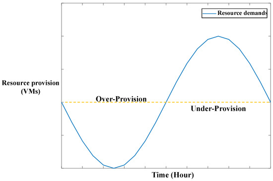
Figure 1.
Situations of resource under- and over-provision. VMs, virtual machines.
To solve these problems, resource managers in cloud computing should allocate resources adaptively, according to the on-demand workload requirements (i.e., adaptive elastic resource allocation). This solution avoids resource over- or under-provision, guarantees QoS, and decreases service costs.
Adaptive elastic resource allocation in cloud computing requires finding the correct amount of computing resources at a given time to automatically meet QoS requirements under variable workloads. The challenge has been addressed in two ways: First, reactive methods, such as those presented in [4,5,6], use pre-defined thresholds to adjust the resources adaptively after a change in workload. Due to the large-scale distributed structure of cloud centers, computing resource schedulers that use these methods may lag behind the workload changes, thus impairing the QoS. Other methods include proactive methods, such as those in [7,8,9], which adjust the resources depending on the predicted future workload. These methods can adapt to the future workload before its occurrence, in order to avoid delays in resource adjustment. However, the workload prediction accuracy impacts the correction of the resource scheduling. Thus, improving the accuracy of such predictions is a key research direction in cloud computing.
Meanwhile, the cost of computing resource management in the cloud is high due to the large-scale distributed structure of cloud centers. Moreover, it is difficult to achieve the real- and small-time granularity requirements for resource scheduling and adjustment. Most popular platforms for infrastructure-as-a-service (IaaS), such as Amazon Web Service, Rackspace, and Aliyun, use one hour as the billing time interval and time granularity. This approach requires building a task processing model in the cloud center using one-hour intervals to obtain a suitable resource size under the optimization objective (e.g., cost or profit optimization). However, real- or fine-time granularity methods cannot solve this problem.
Above all, this study focuses on a proactive method for elastic cloud computing resource allocation, including improving the workload prediction accuracy and designing a resource allocation method. First, based on the proactive method, this study targets the real task arrival workload of the Wikimedia service [10], which is a typical Internet workload, in order to research workload prediction. Then, based on stochastic process and queueing theory, we maximize the cloud service’s profit as the optimization objective to design a computing resource search algorithm. The primary contributions of this study are as follows:
- A novel two-stage adaptive prediction method for Wikimedia workload prediction:
- -
- Introduces first-order gradient features and applies the K-means algorithm to effectively classify workload patterns into uphill and downhill trends, eliminating the need for manual labeling.
- -
- A binary classifier is used for trend categorization, with specialized LSTM networks assigned to each trend category to improve prediction accuracy.
- A queueing theory-based resource allocation algorithm for cloud computing environments:
- -
- Optimizes virtual machine provisioning by incorporating predicted workload patterns, VM rental costs, and task rejection penalties.
- -
- Maximizes service profit while ensuring system stability and QoS guarantees.
- Experimental validation of the proposed proactive resource allocation method:
- -
- Demonstrates improved workload prediction accuracy.
- -
- Identifies the optimal number of VMs required to maximize profit while maintaining QoS constraints.
The remainder of this paper is organized as follows. The related work is summarized in Section 2. Section 3 introduces the system architecture. The prediction method and resource allocation policy are detailed in Section 4 and Section 5, respectively. Section 6 evaluates the performance of the proposed prediction method and resource allocation policy. Finally, Section 7 concludes this paper.
2. Related Work
2.1. Workload Prediction in the Cloud
Due to its crucial role in optimizing resource allocation, workload prediction in cloud computing has attracted substantial research attention. Several studies have focused on support vector regression (SVR), deep learning, and time-series analysis algorithms. These approaches have been shown to enhance system performance through providing highly accurate workload predictions.
In [11], the authors reviewed various traditional methods for cloud computing workload prediction, including SVR, auto-regressive moving average (ARMA), auto-regressive integrated moving average (ARIMA), linear regression (LR), and artificial neural networks (NNs). Based on an ARIMA model, Kumar et al. [12] proposed online computing resource scheduling algorithms. They presented that the QoS is the key element of computing resource allocation in the cloud. Furthermore, Alidoost et al. [13] categorized workloads into distinct types and subsequently applied different ARIMA models to fit each category. Their results demonstrated that this classification approach significantly improves the workload prediction accuracy. Singh et al. [14] used LR, ARIMA, and SVR approaches to predict the cloud service workload. They also classified the workload into distinct types.
Deep learning has been demonstrated to achieve excellent performance in time-series signal fitting and prediction. Islam et al. [15] used an NN to predict the CPU workload, and the NN model outperformed LR in their experiments. Kumar et al. [16] proposed a workload prediction model using an NN and a self-adaptive differential evolution algorithm. With the advancement of deep learning technologies, specialized models, such as recurrent neural networks (RNNs) and LSTM networks, have been specifically designed for processing time-series signals. In [17], a deep learning-based prediction algorithm (L-PAW) utilizing an RNN was proposed for workload prediction in the cloud. RNN-based networks are typically capable of extracting valuable information from input data by continuously updating prior information as it processes the sequence. However, as the time interval increases, the gradients tend to vanish, leading to the gradient vanishing problem. This issue results in ineffective parameter updates within the RNN, limiting its ability to efficiently capture long-term memory dependencies.
To overcome the limitations of RNNs, advanced architectures such as LSTM networks and gated recurrent units (GRUs) have been proposed. The authors in [18] used an LSTM to predict the workload in cloud computing, which outperformed NNs and other traditional methods. Yadav et al. [19] also showed that LSTMs can be effectively adapted for time-series data forecasting, particularly for predicting future server loads in the context of cloud computing.
Additionally, recent research has explored novel approaches for cloud computing workload prediction, especially regarding the Transformer architecture. For instance, Morichetta et al. [20] applied the Transformer architecture for time-series prediction in cloud computing. Their experimental results demonstrated that the Transformer-based approach achieved competitive performance through effectively modeling temporal workload patterns. Furthermore, the authors of [21] evaluated the Transformer architecture against other approaches for cloud workload prediction, and their comparative analysis revealed that the Transformer architecture is particularly suitable for workload forecasting. Building upon the Transformer architecture, several advanced models have been proposed. Cao et al. [22] introduced a hybrid LSTM–Transformer model for multi-task time-series forecasting. Although the Transformer model has a good capability for time-series forecasting, the experiments reported in [21] revealed that its performance is inferior to that of LSTM, particularly when considering single-task scenarios, limited training data conditions, and short-term predictions. Thus, LSTM demonstrates superior performance in single-task scenarios, particularly for short-term time-series prediction.
Neither LSTM nor Transformer architectures, as standalone models, are likely to achieve optimal prediction performance when addressing complex, volatile, and seasonally varying workloads in cloud computing. To overcome these limitations, some researchers have employed multiple models for workload prediction. The multi-model approach categorizes workloads into different groups and applies corresponding sub-models to predict the workload for each category. In [23], based on a normality test, the workload was divided into two categories: if the workload satisfied the normality test, ARIMA was used to predict the CPU workload; otherwise, NNs were applied. Similarly, the authors in [24] divided the resource usage of tasks into different categories according to the priorities and change rates of the tasks. They employed SVR and LR models to predict workloads for different categories. The results showed that multiple models can achieve higher prediction accuracy than a single model.
However, few studies have focused on multiple model-based methods. Additionally, the CPU workload must be predicted for each VM in the cloud center if predictions are processed using CPU workload information. As the number of VMs increases, the workload prediction task requires significantly more computing resources. Apart from CPU workload prediction, the task arrival workload can represent the task workload directly and reduce the prediction cost using the center node, which avoids the need for workload prediction regarding the distributed VMs in the cloud center. Thus, we focus on task arrival workload prediction, which represents a typical single-task forecasting problem. In contrast to one-step prediction, which utilizes actual historical data, multi-step prediction relies on uncertain forecasted values as inputs. Moreover, the additional predictions in multi-step forecasting offer limited practical value for cloud resource scheduling. Consequently, our focus is on short-term predictions, as the immediate forecast has a more direct and actionable impact on resource allocation. While LSTM has demonstrated strong performance in short-term, single-target time-series forecasting, due to the limitations of single models in capturing the complex patterns of volatile and seasonally varying workloads, we adopted a multi-model approach to predict the number of arriving tasks. Yet several key challenges remain, listed below:
- (1)
- The task arrival workload only contains numerical information, and classifying the workload adaptively is the key problem.
- (2)
- Due to different workload categories, building sub-training data sets for training of the corresponding sub-models is another key problem.
To address the challenges above, we propose a method involving multiple models based on an LSTM that can adaptively classify the workload into suitable categories and predict the workload using the corresponding sub-prediction model. Furthermore, to minimize the human and material costs associated with manually annotating two-category sub-training data sets, we propose an unsupervised machine learning method that utilizes workload trend features to automatically generate sub-training data sets for the sub-prediction model.
2.2. Queueing Theory in Cloud Computing
Queueing theory [25] is a useful tool for analyzing task processing in the cloud center context, which has been used to analyze the waiting time, task dropping, resource utilization, queueing length, and other aspects. Xia et al. [26] used a queueing model to evaluate the expected request completion time, rejection probability, and system overhead rate of VM scheduling and request handling process. Kushchazli et al. [27] leveraged a queuing-based model to study VM migration dynamics, offering insights into resource optimization, task processing, and performance metrics. In [28], the authors highlighted the crucial role of the queuing theory in cloud computing through integrating the M/M/c/K queuing model with the improved dynamic Johnson sequencing algorithm (DJS) to optimize task scheduling and resource allocation. Wei and Liang [29] employed a multi-queuing model to analyze and optimize edge server load percentages in mobile cloud computing, minimizing the task response time while ensuring fairness in offloading delays. In [30], the authors modeled fog devices as M/M/1 queues and cloud systems as M/M/C queues. To address the fog–cloud workload distribution problem, the NSGA-II algorithm was employed, with the objective of minimizing both energy consumption and system delays.
These previous studies demonstrated that queueing theory can be used to model a cloud service and examine the performance of task processing in cloud computing. Importantly, the queueing model can also be used to optimize resource management. In practice, due to the constraints of load monitoring and the minimum resource rental time interval (at least one hour), real- or fine-time granularity methods cannot be used to analyze task processing in the cloud directly. Hence, we used stochastic queuing theory to model task processing in the context of cloud computing in one-hour intervals, in order to optimize the management of computing resources. However, mathematical analysis is required to study how to transmit the predicted value to suitable cloud resources using the stochastic queueing model. Thus, one of the key contributions of this study is presenting a detailed mathematical model of the process.
3. System Architecture
The cloud platform architecture is shown in Figure 2.

Figure 2.
The resource management architecture in cloud computing. IaaS, infrastructure-as-a-service. VMs, virtual machines.
The main components of a cloud platform are as follows:
- Cloud resource pool—This component is composed of VMs that run in the physical server cluster. Based on virtual technologies, the computing resources of a VM (e.g., CPU, memory, disks, and networking) can be configured on demand. The resource pool also can be considered as an IaaS layer, which provides online computing resources.
- Task scheduling and networking interface—This component provides load balancing for the tasks that arrive from the Internet. Some studies, such as [31,32,33], have researched task scheduling optimization policies. Unlike these studies, we did not focus on task scheduling in the cloud center. Instead, we used a common load-balancing policy (i.e., round-robin; RR) as a task scheduling policy, meaning that the tasks are distributed evenly across the VMs.
- Cloud management platform—This component provides the resource management service in the cloud center. The admission control service and the resource monitoring service collect the resource pool running information (e.g., resource utilization of physical servers and VMs, the health status of physical servers, and hardware configurations). This collected information is stored in the database and used by the resource scheduling service to identify the suitable target physical server for launching the VM. The admission control component authenticates cloud center administrators and manages VM lifecycle operations, specifically handling requests for VM provisioning and de-allocation.
As in [34], the cloud management platform with elastic resource management has the following external components:
- Workload monitoring—This component provides the workload information collection service. In general, the workload monitoring component can periodically collect the task arrival workload information through the load-balancing interface.
- Workload prediction—Based on historical information, this component predicts the future workload.
- Resource determination—Based on a specific optimization objective (e.g., cost or profit optimization), this component determines the suitable number of VMs according to the predicted future workload. When the resource determination result is obtained, the component sends to the VM control a command to launch or release the corresponding number of VMs.
Based on the architecture detailed above, this study examines key technologies for workload prediction and resource determination.
4. Prediction Method
4.1. Introduction of Workload Prediction
Workload prediction can be modeled as a regression and fitting problem for a time-series signal. The historical signal is used to calculate the signal value at the next time slot. Let be the historical workload values from the time slot to the time slot. The prediction value at the time slot can be presented as follows:
where is a regression and fitting function that represents the relationship between historical and predicted values.
As mentioned in Section 2, the LSTM was shown to outperform other methods in short-term single-task time-series forecasting in previous research. In an LSTM, the output value of each gate is determined by the weighted sum of the current input and past state values. The weighted information can be updated in a self-loop, according to the structure of LSTM. Thus, LSTM becomes more effective in accessing past information. In the self-loop structure, each unit can receive previous information to perform a specific operation and output the results to the next unit. An LSTM unit is shown in Figure 3.

Figure 3.
Architecture of a long short-term memory unit.
In an LSTM, each gate can be presented as an activation function, σ(·), such as the sigmoid, ReLU, or tanh function. Let and be the current input and past state output, respectively. The LSTM can be expanded following the time-series as a sequential connection from a past state to the current state. The key component of an LSTM is a cell, which is used to store the past state and determine the amount of past state information. According to Figure 2, the value of input gate and block input in an LSTM can be calculated as follows:
where , , and are the bias, weight of the input, and recurrent state weight in the input gate, respectively; similarly, , , and are the bias, weight of the input, and recurrent state weight in the block input, respectively. In an LSTM, the output of the forget gate controls the recurrent memory state of the cell, which is influenced by and . The output of the forget gate can be calculated as follows:
According to the calculations above, the state of the cell is updated as follows:
The value of the output gate can be calculated as follows:
Finally, the output of the LSTM can be calculated as follows:
A prediction model based on an LSTM is shown in Figure 4. In this model, the LSTM layer is used to extract time-series features, which capture both past and present temporal information. The output layer of the LSTM is a fully connected structure, and its output can be calculated as follows:
where and denote the weight and bias of the output layer, respectively.

Figure 4.
Architecture of a long short-term memory (LSTM) prediction model.
To prevent the gradient from becoming large and to accelerate the training process, the input of the network needs to be normalized. Max–min normalization is as follows:
where and are the original workload data and normalized value at the time slot, respectively, and and denote the minimum and maximum values in the input data set, respectively.
4.2. Adaptive Two-Stage Multi-Neural Network Based on the LSTM Prediction Method
In this study, we focus on prediction of the task arrival workload in the Wikimedia service, as shown in Figure 5. The workload trace of the Wikimedia service contains the number of received HTTP requests, aggregated into one-hour intervals.
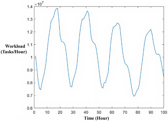
Figure 5.
Task arrival workload of the Wikimedia service.
As mentioned in Section 2, multiple-model methods can classify the workload into suitable categories and use different prediction models to fit the different categories of the workload, according to the workload’s characteristics. Although the workload presents some randomness with increasing and decreasing values, we can classify the workload into two categories—namely, uphill (workload increasing) and downhill (workload decreasing)—as shown in Figure 6.

Figure 6.
Classification of the task arrival workload for the Wikimedia service.
Based on the classification results shown in Figure 6, we propose a new workload prediction method, named the adaptive two-stage multi-neural network model based on LSTM (ATSMNN-LSTM). The structure of the ATSMNN-LSTM is shown in Figure 7.

Figure 7.
Architecture of the proposed adaptive two-stage multi-neural network model based on long short-term memory (ATSMNN-LSTM) method.
The proposed workload prediction method contains two main processes: (1) an adaptive classification process, which uses an NN for binary classification to classify the workload input data into the uphill or downhill category, according to the workload change trend; and (2) a classification prediction process, in which, according to the workload classification results, the workload input data are routed to the corresponding sub-prediction model (e.g., uphill LSTM or downhill LSTM model) to predict the future workload.
According to Figure 7, the workload classification task poses the following challenge: an NN for binary classification and two LSTM prediction models must be trained. However, the task arrival workload only contains time and numerical information and, so, it is difficult to build sub-training data sets for the two considered categories (i.e., uphill and downhill data sets) and label the two-category workload training data set for model training. The manual annotation method for building the two category sub-training data sets and labeling the two-category workload requires significant human and material resources. Thus, unsupervised machine learning is a suitable method for this problem. The k-means algorithm [35] is a typical unsupervised clustering algorithm, which uses the Euclidean distance—defined as , where i and j are the labels of the and categories, respectively—to cluster the data into different categories.
In Figure 8, three groups of workload data are shown, denoted as G1, G2, and G3. Here, G1 and G3 are uphill categories, while G2 is the downhill category. Figure 8 shows that the maximum distance between G1 and G2 () is smaller than that between G1 and G3 (). Due to the use of the Euclidean distance as the clustering metric in the k-means algorithm, G1 and G2 might be grouped into the same cluster, while G1 and G3 could be assigned to different clusters. This may confuse the k-means algorithm when working with the original data. Therefore, a feature that represents the workload change trend is needed.

Figure 8.
Euclidean distances of three workload data groups.
Based on Figure 8, we consider that the first-order gradient can effectively represent the workload change trend. The first-order gradient feature at time slot in a discrete-time system can be calculated as follows:
where is the time interval between two adjacent time points for workload data collection. In the Wikimedia service, the time interval is 1 h; that is, the workload data collection period . Based on Figure 8, the first-order gradient feature of the workload is shown in Figure 9.

Figure 9.
First-order gradient features of three workload data groups.
As shown in Figure 9, when , the workload change trend is uphill; meanwhile, when , the workload change trend is downhill. If the workload input data are , the first-order gradient vector can be calculated as follows:
Accordingly, when the workload change trends of G1 and G3 are positive, their first-order gradient vectors are positive. Thus, k-means can classify G1 and G3 into the uphill category. As the workload change trend of G2 is negative, its first-order gradient vector is negative. The k-means algorithm classifies G2 into the downhill category, which is different from G1 and G3. Thus, the first-order gradient feature can be effectively used for k-means classification.
Based on the two training subsets (i.e., the uphill and downhill training data sets), built using the k-means algorithm with the first-order gradient feature, we need to train a binary classification model to classify the workload according to the workload change trend and two LSTM prediction models to predict the uphill and downhill category workloads. We use an NN for binary classification to process the workload classification, the architecture of which is shown in Figure 10.

Figure 10.
Architecture of the binary classification neural network model.
The input data of the binary classification NN model are the first-order gradient vector, the hidden layer has a fully connected structure, and the output layer has two cells. The values of the two output cells present the probabilities (i.e., the degree of confidence) of the uphill and downhill categories, respectively. To differentiate between the results, the output layer values are normalized, setting the maximum value to 1 and the minimum value to 0.
The training process of the proposed workload prediction model is shown in Figure 11.
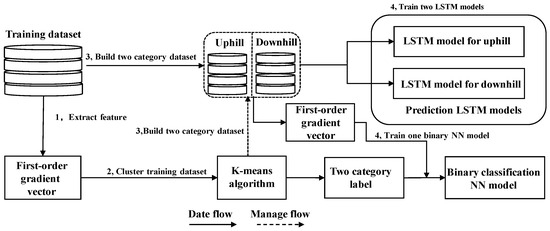
Figure 11.
Training process of the proposed prediction model. LSTM, long short-term memory; NN, neural network.
The training process includes four steps: (1) the first-order gradient vector is extracted from the workload training data set; (2) using the first-order gradient features, the K-means algorithm clusters the workload training data set; (3) according to the K-means clustering results, the workload training data set is classified and labeled into two categories (i.e., uphill category data set and downhill category data set); and (4) with the categorized training data sets and their corresponding labels, the two sub-LSTM prediction models and one binary classification NN model are trained using the stochastic gradient descent method.
After model training, the workflow of the proposed workload prediction method (i.e., ATSMNN-LSTM) is shown in Figure 12.

Figure 12.
Workflow of the proposed workload prediction method. LSTM, long short-term memory; NN, neural network.
The prediction procedure of the proposed model involves four steps: (1) the workload monitoring service in the cloud management platform collects the workload data and triggers the workload prediction process periodically; (2) if the workload prediction process is triggered, the first-order gradient vector is extracted according to the historical data sequence; (3) based on the first-order gradient vector, the binary NN classification model classifies the workload into the uphill or downhill category; and (4) the input workload data are routed to the corresponding sub-LSTM prediction model to predict the workload for the next time slot.
5. Cloud Resource Allocation Policy Based on Maximum Cloud Service Profit
5.1. Task Processing Modeling in the Cloud Service
As shown in Figure 2, the cloud resource pool is composed of VMs. Each VM in the resource pool is run in a target physical server, and the computing resources of the VM are abstracted by the virtualization layer and presented as vCPU, vMemory, and vNetwork, as shown in Figure 13. When a task arrives at the VM, it is buffered and queued in the memory of the VM. Next, the tasks are processed by the vCPU according to the first-in-first-out (FIFO) service policy. If the task cannot be completed within the deadline, it will be dropped from the VM.

Figure 13.
Structure of the task processing queueing model in virtual machines (VMs).
To obtain enough revenue, most cloud services, such as AWS, Rackspace, and Aliyun, schedule resources and set the billing interval to one hour, which is the same as the workload monitoring interval. Thus, some methods based on a real-time queueing model or a short time slot may not be suitable for cloud center resource management. Based on previous research [36,37,38,39], although the workload of the Wikimedia service does not follow the homogeneous Poisson distribution in one-hour intervals, the workload with a small time slot of one hour follows a uniform Poisson distribution. Let denote a small time slot of one hour. Based on the theoretical analyses in previous research [40,41], we assumed that the task length (i.e., the instruction length) follows an exponential distribution, which can be obtained from the statistics of historical tasks completed by the cloud service. Therefore, the task execution time also follows an exponential distribution. Overall, in a small time slot , the task process in the VM can be presented using the M/M/1/K queueing model, which follows the first-come-first-served policy. In the M/M/1/K model, “1” represents one processing unit (i.e., one VM has one vCPU), and K represents the task queueing length. If the task queueing length exceeds K, the task will be lost. According to the QoS deadline, K can be calculated as follows:
where is the maximum allowed processing time of the task, which is the maximum allowed processing time interval between the time when the task arrives at the VM and its deadline, and is the average task execution time in the vCPU.
According to the average task execution time (i.e., ), the average number of tasks that are processed by the vCPU of the VM in time slot can be calculated as follows:
The system load of the VM in time slot can be calculated as follows:
where is the task arrival rate in time slot . The task loss ratio of the model can be calculated as follows:
Thus, in time slot , the actual task arrival rate (i.e., the average number of task arrivals) of the VM is as follows:
Furthermore, the average number of lost tasks can be calculated as
Thus, the actual system load is as follows:
The average task response delay in time slot is calculated as follows:
According to Figure 2, the cloud service contains a load-balancing service and computing resources. The load-balancing service schedules tasks following a specific policy. In general, the most frequently used policy in the load-balancing service is RR, which uses a circular strategy to schedule a task for each VM in the cloud service. When the task arrival number in time slot is and the number of the VMs in time slot is , the task arrival number of each VM in time slot is calculated as follows:
Notably, is the mean value in the stochastic process, while the values in Equation (20) are actual numbers. Thus, cannot be used in the model directly. With the interval , 1 h can be divided into small time slots, where . As mentioned before, a workload with a small time slot of 1 h follows a uniform Poisson distribution. According to the ergodic process in stochastic Poisson process theory, the average task arrival number in small time slot is approximately equal to , which can be calculated as follows:
5.2. Maximum Cloud Service Profit Resource Allocation Method
Let represent the VM rental cost () and task profit (). The cloud service profit in time slot can be calculated as follows:
where represents the total task profit per VM in time slot , is the task profit loss of each VM in time slot , and is the rental cost of each VM in time slot . Thus, the term represents the cloud service profit of each VM in time slot .
In the cloud service, the profit of a service is important for the development of the Internet. Thus, maximization of the profit of the service is the optimization objective considered in this study; that is, the cloud service profit is used as the optimization objective. Additionally, we also need to guarantee the QoS provision (i.e., deadline requirements) and system stability. Thus, the optimization objective is presented as follows:
where is the maximum allowed processing time of the task, and is the maximum allowed system load of a VM.
In Equation (23), denotes the arrival rate from the Internet; therefore, is a determined number that cannot be affected by the system. Thus, the cloud service profit is affected by the task loss and VM rental costs (i.e., the cloud service costs). The objective in Equation (23) can be transferred to minimize the cloud service costs as follows:
Notably, the convex property of Equation (24) is also affected by the task loss and VM rental costs. It is assumed that , the average task execution time is , and the maximum allowed processing time for a task is . According to Amazon’s VM rental price, the rental cost of a VM is RMB 1.2179 per hour. There are three cases with different task profits, as follows:
- (1)
- High task profit: Due to the typical high load of the Wikimedia service (the workload of the task arrival can be on the order of ), we first assume that the task profit is RMB 0.01. Thus, the task loss becomes the main element that affects the cloud service cost, rather than the rental cost of VM. To reduce the cloud service cost, we need to allocate enough VMs to reduce the cost of task loss. Thus, the cloud service cost decreases rapidly when the number of VMs increases. When the number of VMs becomes redundant, the cloud service cost increases slowly. The cloud service cost is a weakly convex function, as shown in Figure 14.
 Figure 14. Cloud service costs with a high task profit. VM, virtual machine.
 - (2)
- The low task profit: We next assume that the task profit is 0.0000001. Thus, the rental costs of VMs become the main element affecting the cloud service cost. In this case, the optimization resource allocation strategy uses the smallest number of VMs; that is, one VM. Thus, the cloud service cost is a monotonic increasing function, as shown in Figure 15.
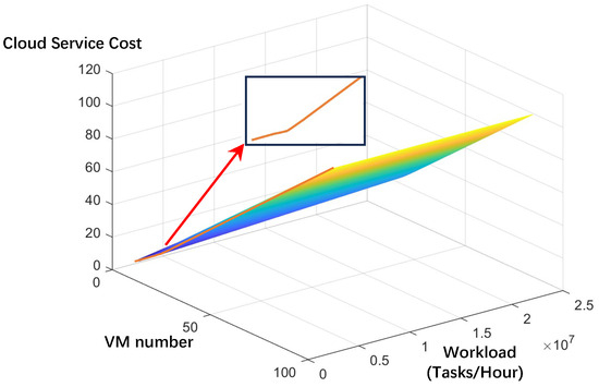 Figure 15. Cloud service costs with a low task profit. VM, virtual machine.
 - (3)
- The medium task profit: Compared to the previous two cases, we then assume that the task profit is 0.00001, which means that the task profit and the rental costs of VMs both affect the cloud service cost. In this case, when the number of VMs increases, the task loss decreases but the rental costs of VMs increase, and vice versa. Thus, Equation (24) becomes a strongly convex function, as shown in Figure 16.
 Figure 16. Cloud service costs with a medium task profit. VM, virtual machine.
As mentioned above, the maximum cloud service profit resource allocation (MaxCSPR) algorithm is proposed to find a suitable number of VMs, according to the workload requirements. The details of the MaxCSPR algorithm are shown in Algorithm 1.
| Algorithm 1 MaxCSPR algorithm |
| Input: The task arrival in the time slot; The cloud service cost vector ; The average task execution time ); The allowable process time of the task ); The allowable system load of VM ); The maximum number of VMs allowed ). |
|
To fit the above three cases, MaxCSPR includes the increasing and decreasing search processes for the cloud resources. When the cost increases with an increasing number of VMs, the number of VMs should be decreased, and vice versa. Furthermore, the proposed algorithm sets the minimum resource size to 1, in order to avoid empty cloud resources. Similarly, the maximum resource size is set as .
To achieve proactive elastic resource allocation in the cloud, the ATSMNN-LSTM workload prediction method is combined with the MaxCSPR algorithm. In the proactive elastic resource allocation method, the workload prediction result—namely, —is used as the time slot input to the MaxCSPR algorithm, which allows the MaxCSPR algorithm to schedule VM resources for the time slot. In this study, the algorithm combining the ATSMM-LSTM and MaxCSPR is named the maximum cloud service profit resource search algorithm based on network workload prediction (MaxCSPR-NWP).
6. Performance Evaluation
6.1. Experimental Environment Settings
The workload data set was collected from real data traces of the Wikimedia web service, with each data trace containing the number of tasks that arrived per hour. The data set contained data for approximately 40,000 h; of these, 70% were used as a training set, and 30% as a test set. Additionally, the historical data had an input of size 6, and the LSTM layer contained 25 cells.
To evaluate the performance of the proposed prediction method, we used the following three metrics:
- (1)
- Mean absolute percentage error (MAPE) [42]:where is the size of the data set, is the prediction result, and is the real data. A lower MAPE indicates a better prediction result.
- (2)
- R-squared () [43]:If the value is close to 1, the prediction model fits better.
- (3)
- Root-mean-squared error (RMSE) [44]:A lower RMSE indicates a better prediction result.
6.2. Prediction Performance Evaluation
To evaluate the performance of the proposed prediction method, we compared it to other prediction models, including ATSMNN (which uses an NN instead of the LSTM used in ATSMNN-LSTM), LR, ARIMA, SVR, LSTM, Transformer, LSTM–Transformer, and NN. The prediction results for 30 randomly selected time points are shown in Figure 17.

Figure 17.
Comparison of the prediction results for 30 time points.
From Figure 17, all prediction methods fitted the workload trend, which means that the ATSTMNN-LSTM and other methods could effectively predict the workload trend.
To demonstrate that ATSMNN-LSTM can obtain a higher prediction accuracy, we compared the metrics used for assessment of the workload prediction using the different methods, as shown in Table 1.

Table 1.
Workload prediction metrics for different models.
According to Table 1, the RMSE and MAPE values obtained with ATSMNN-LSTM (3.7805 and 0.0276, respectively) were lower than those of other models. Moreover, the of the ATSMNN-LSTM model was 0.9522, which was closer to 1 and higher than those of the other models, demonstrating that the ATSMNN-LSTM had improved prediction performance. ATSMNN-LSTM achieved better prediction accuracy than a single LSTM or an NN. Furthermore, due to the high prediction accuracy of the LSTM, the prediction results of ATSMNN-LSTM were better than those obtained with the ATSMNN model. Moreover, the performance of the Transformer model was better than that of the ARIMA, SVR, LR, and NN models, demonstrating that the Transformer model is more suitable for time-series forecasting compared to traditional approaches. However, the experimental results indicated that the Transformer model did not outperform the LSTM in terms of prediction accuracy. Although the Transformer exhibited excellent performance in sequence processing, its complex model architecture is prone to overfitting when using limited data and presents training difficulties. For the Wikimedia workload time-series used in this study, the Transformer may not outperform the LSTM in terms of single-task, short-term prediction performance. This finding aligns with the conclusions reported in [21]. Additionally, the experimental results indicated that the LSTM–Transformer model did not achieve high performance. Although the LSTM–Transformer model enhances the Transformer architecture by incorporating LSTM modules, it further increases the model complexity, leading to greater training difficulties and a higher risk of overfitting.
To present the details of the prediction graphically, we compare the relative error () and absolute error () at 70 time points in Figure 18 and Figure 19, respectively.

Figure 18.
Comparison of the relative error (RE).

Figure 19.
Comparison of the absolute error (AE).
As shown in Figure 18 and Figure 19, compared to the other models, ATSMNN-LSTM guaranteed low and stable relative and absolute errors. Additionally, we show the cumulative distribution percentage error in Figure 20, where the X-axis indicates the percentage of the error threshold (PET), while the Y-axis indicates the percentage of prediction values below the error threshold percentage (PBET).

Figure 20.
Cumulative distribution percentage error for different models. ET, error threshold; PBET, error threshold percentage.
According to Figure 20, the cumulative distribution percentage error of ATSMNN-LSTM was higher than that of other models at PBET values less than 60%. Thus, the prediction error of ATSMNN-LSTM was mostly between 0% and 60%, and its number of high prediction errors (i.e., 60–100%) was lower than that of the other models. Furthermore, when the cumulative distribution percentage error of the ATSMNN-LSTM decreased, the interval of the cumulative distribution percentage error between ATSMNN-LSTM and the other models increased. Thus, the number of small error prediction results of ATSMNN-LSTM is larger than that of the other models. These results prove that ATSMNN-LSTM achieved higher prediction accuracy in the comparison.
To demonstrate the superior performance of ATSMNN-LSTM over other models, we employ the Diebold–Mariano (DM) test statistics [45] to compare the statistical significance of prediction errors across different models, as illustrated in Figure 21. The corresponding p-value for ATSMNN-LSTM is provided in Table 2.

Figure 21.
Heatmap of the Diebold–Mariano (DM) test statistics.
Table 2.
The p-value of ATSMNN-LSTM model.
The Diebold–Mariano (DM) test statistic matrix quantifies pairwise predictive accuracy differences between models, where each off-diagonal element represents the DM statistic for a row-versus-column model comparison. Positive values indicate superior performance of the column model, while negative values favor the row model. Larger absolute values reflect stronger statistical significance. A p-value < 0.05 suggests a statistically significant difference in prediction errors.
As shown in Figure 21, the test results for ATSMNN-LSTM compared to other models are consistently negative (first row: −4.918, −15.41, −5.947, −60.67, −4.444, −6.93, −7.063, −6.315), indicating that this model outperforms others in prediction accuracy. Combined with the statistical significance (p-value < 0.05) shown in Table 2, these results demonstrate that ATSMNN-LSTM achieves statistically significant improvements in prediction accuracy over all comparative models.
Additionally, to present the effectiveness of the proposed k-means method with the first-order gradient feature, we randomly selected two groups of the classification NN output data under the first-order gradient feature and original data, respectively. The results are compared in Figure 22 and Figure 23.

Figure 22.
Binary classification neural network outputs with the first-order gradient feature.
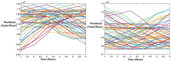
Figure 23.
Binary classification neural network outputs with the original data.
The two upper figures demonstrate that the NN with the first-order gradient feature classified the data into suitable categories (i.e., uphill and downhill categories). Moreover, this proves that the k-means algorithm with the first-order gradient feature is effective in automatically building a training data set for the NN, thus avoiding the costs associated with manual labeling of the training data.
Robustness Analysis:
The ATSMNN-LSTM model partitions the data into uphill and downhill trends, isolating more consistent patterns and reducing the impact of anomalies, particularly those deviating from the overall trend, on model performance. The specialized LSTM models, each trained on specific trend patterns, effectively mitigate the impact of outliers by constraining anomalous fluctuations within their respective trend categories, thereby reducing the interference of extreme values on prediction performance. Moreover, the LSTM architecture employed in the ATSMNN-LSTM model offers inherent resilience to outliers through its gating mechanisms. Specifically, the forget gate adaptively modulates the weights of anomalous values, while the memory cell maintains the intrinsic trend characteristics, ensuring prediction stability even in the presence of transient load fluctuations. Thus, the ATSMNN-LSTM model exhibits enhanced robustness.
6.3. Resource Allocation Performance Evaluation
To evaluate the VM allocation performance of the MaxCSPR algorithm, the parameters were set as follows: , average task execution time = 5 ms (i.e., the processing ability of the VM was 1000 MIPS (million instructions per second, MIPS) and the average task instruction length was 5 million instructions), maximum allowed processing time of the task = 100 ms, and maximum system load = 90%. According to the AWS price list, the rental cost of a VM was set as 1.1279 RMB/h, and the profit of a task was 0.00001. Based on the ergodic process and the definition of the Poisson distribution, the task arrival rate of each was calculated using Equations (20) and (21). The task arrival number was generated from the Poisson distribution according to the task arrival rate.
First, we compared the performance of the MaxCSPR algorithm with that of other algorithms. Generally, the on-demand and elastic allocation of cloud resources improves task processing and QoS; for example, this was the case for the algorithms presented in [46]. These resource allocation and scheduling algorithms, which take the QoS guarantee as a target, can be called QoS guarantee (QoS-G) algorithms. To evaluate the service loss (S.Loss), system load (S.Load), and service delay (S.Delay) in the MaxCSPR algorithm, we compared the performance of MaxCSPR and QoS-G, as shown in Figure 24, Figure 25 and Figure 26.
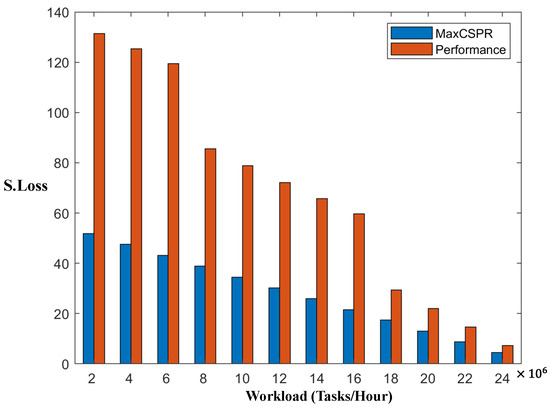
Figure 24.
Cloud service loss (S.Loss) of the MaxCSPR and QoS-G algorithms.

Figure 25.
Virtual machine system load (S.Load) of the MaxCSPR and QoS-G algorithms.

Figure 26.
Average task delay (S.Delay) of the MaxCSPR and QoS-G algorithms.
According to Figure 24, the QoS-G algorithm takes the QoS guarantee of the tasks as the target and does not consider the best match between the number of VMs and task profit, while MaxCSPR takes the minimum cloud service loss as the target; thus, MaxCSPR can minimize the cloud service loss. Therefore, MaxCSPR can improve the profit of the cloud service.
Figure 25 shows that MaxCSPR minimizes the cloud service loss as the target and considers the system stability (i.e., the upper limit of the VM system load); thus, MaxCSPR can guarantee that the cloud server load is lower than the required upper cloud server load limit (90%), which guarantees system stability.
According to Figure 26, although QoS-G can guarantee the QoS of the task (i.e., the average task delay is lower than 100 ms), QoS-G does not consider the stability of the VM system. Therefore, the VM system load of QoS-G may be higher than 90%, which can lead to VM overloading or software errors. Additionally, Figure 25 shows that the average task delay of QoS-G is higher than that of MaxCSPR. This is because MaxCSPR not only considers the QoS of the task, but also the stability of the VM system. Thus, MaxCSPR can guarantee that the VM system load does not exceed the allowed upper system load and allocates the optimal number of VMs in the cloud center to avoid an overload of tasks to be processed by a few VMs. However, QoS-G only considers the QoS of the task. Therefore, if the VM can satisfy the average delay requirement for tasks, these tasks will be scheduled to a few VMs, increasing the average task delay compared to MaxCSPR.
Overall, MaxCSPR can guarantee the system’s stability and the QoS of the task better than QoS-G. Importantly, MaxCSPR can improve the profit of the cloud service, which proves the effectiveness of design requirements and theoretical analysis.
6.4. MaxCSPR with Workload Prediction Evaluation
To analyze how different workload prediction methods impact the performance of the MaxCSPR algorithm, we compared the number of VMs required by MaxCSPR under different prediction methods to that under the real workload. The results are compared in Table 3.
Table 3.
Metrics of virtual machine allocation using different workload prediction methods.
According to Table 3, due to the high prediction accuracy of the ATSMNN-LSTM algorithm, its prediction error for the VM number compared to the real workload was improved, in terms of the MAPE and RMSE values (0.0276 and 0.7719, respectively). Moreover, the was better for ATSMNN-LSTM (0.9356) than for the other prediction methods. Thus, the prediction method is a key element that impacts the resource allocation accuracy of the proactive method in the cloud computing context. The results demonstrate that MaxCSPR-NWP can obtain higher accuracy regarding allocation of the number of VMs. Meanwhile, Figure 27 shows that the VM number can be allocated in an elastic and online manner, according to the change in the workload.

Figure 27.
Virtual machine (VM) number allocation using the MaxCSPR algorithm.
To evaluate the performance of the MaxCSPR algorithm in a real system, we used CloudSim [47] to conduct a simulation experiment. This simulation system can be considered as a real-time queueing serve system (i.e., a real-time model) with first-come-first-served policy in the cloud center. Based on the definition of the ergodic process in Poisson processes, the workload in a small time slot can be generated using Equations (20) and (21), and the average task processing time was 5 ms (i.e., the MIPS of each VM was 1000 and the average instruction length was 5 million instructions), and the task length was generated using the exponential distribution with the mean value (5 million instructions). The average task delay (AT.Delay) and VM system load (VS.Load) in the CloudSim simulation are shown in Figure 28.

Figure 28.
Average task delay (AT.Delay) and virtual machine (VM) system load (VS.Load) in CloudSim simulation.
According to Figure 28, the VM system load of the MaxCSPR-NWP algorithm was below 90%, indicating the stability of the VM system. Moreover, the VM system load was higher than 70%, which means that the computing resource (CPU) and cloud rental costs were used effectively. In this figure, the trend of the VM system load and average task delay are the same (i.e., when the VM system load was small, the workload of the task arrival was small and the average task delay was small, and vice versa). Notably, the average task delay and VM system load were concentrated in a stable interval as VMs can be allocated online and on demand, according to the change in workload. Moreover, the cloud service can guarantee the QoS requirements; namely, the average task delay was lower than 100 ms. Overall, the results demonstrate that the proposed proactive cloud resource allocation method—that is, the MaxCSPR-NWP algorithm—guarantees both the QoS requirements and VM system stability, while also optimizing the effective usage of cloud resources and improves the profit of the cloud service.
Implementation Challenges and Engineering Analysis:
Current cloud service providers have implemented various approaches to predictive elastic resource scheduling, each facing distinct technical challenges in practical deployments: (1) AWS: limited workload prediction accuracy in predictive scaling mechanisms due to reliance on conventional machine learning models. (2) Rackspace: fragmented resource orchestration in hybrid cloud architectures, which hinders the efficiency of multi-cloud deployments. (3) Aliyun: suboptimal cost-performance trade-offs in intelligent scheduling, particularly under dynamic workload conditions. Our methodology systematically addresses these challenges by enhancing workload prediction accuracy through adaptive multimodal prediction techniques, improving resource orchestration via unified abstraction frameworks, and optimizing cost-performance trade-offs using dynamic adaptation strategies. This comprehensive approach not only resolves existing implementation limitations but also provides a foundation for more efficient elastic resource management in cloud environments.
7. Conclusions
In this study, we investigated resource allocation in the context of cloud computing. To match the resource requirements with changes in workload, we proposed a proactive cloud resource allocation method to schedule the cloud resources elastically and on demand. First, to improve the prediction accuracy, we proposed a new workload prediction model, which we called the adaptive two-stage multi-neural network based on LSTM (ATSMNN-LSTM). The proposed method can adaptively classify the workload into two categories (i.e., uphill and downhill), according to the workload trend. Next, according to the workload classification results, the workload prediction process is routed to the corresponding LSTM prediction sub-model. Furthermore, to avoid the cost of manual annotation in building the training data set, we use the first-order gradient feature and the unsupervised k-means algorithm to cluster and label the original training data into two training subsets (i.e., uphill and downhill data sets) for training of the NNs. Based on the queueing theory, the cloud service was modeled using a comprehensible mathematical description. With the target of the maximum cloud service profit, VM system load, and QoS requirements, we proposed a cloud resource scheduling algorithm to find an optimal number of VMs for the cloud center, in accordance with the predicted workload. The experimental results demonstrated that the proposed cloud resource allocation method not only achieves a high workload prediction accuracy but can also elastically allocate and schedule the cloud resources to match the workload requirements under QoS and VM system load requirements.
Author Contributions
Conceptualization, L.L.; Methodology, L.L.; Software, L.L.; Writing—original draft, L.L.; Writing—review and editing, X.G.; Funding acquisition, X.G. All authors have read and agreed to the published version of the manuscript.
Funding
This study was funded by Guangdong Science Technology Project (GDSTP: 2017A010101027) and the National Natural Science Foundation of China (NSFC: 61936003).
Institutional Review Board Statement
Not applicable.
Informed Consent Statement
Not applicable.
Data Availability Statement
The original contributions presented in this study are included in the article. Further inquiries can be directed to the corresponding author.
Conflicts of Interest
The authors declare no conflict of interest.
References
- Goel, P.K.; Gulati, S.; Singh, A.; Tyagi, A.; Komal, K.; Mahur, L.S. Energy-Efficient Block-Chain Solutions for Edge and Cloud Computing Infrastructures. In Proceedings of the 2024 2nd International Conference on Disruptive Technologies (ICDT), Greater Noida, India, 15–16 March 2024; IEEE: Piscataway, NJ, USA, 2024; pp. 852–856. [Google Scholar] [CrossRef]
- Ismahene, N.W.; Souheila, B.; Nacereddine, Z. An Auto Scaling Energy Efficient Approach in Apache Hadoop. In Proceedings of the 2020 International Conference on Advanced Aspects of Software Engineering (ICAASE), Constantine, Algeria, 28–30 November 2020; IEEE: Piscataway, NJ, USA, 2020; pp. 1–6. [Google Scholar] [CrossRef]
- Amiri, M.; Mohammad-Khanli, L. Survey on prediction models of applications for resources provisioning in cloud. J. Netw. Comput. Appl. 2017, 82, 93–113. [Google Scholar] [CrossRef]
- Khan, A.A.; Vidhyadhari, C.H.; Kumar, S. A review on fixed threshold based and adaptive threshold based auto-scaling techniques in cloud computing. MATEC Web Conf. 2024, 392, 01115. [Google Scholar] [CrossRef]
- Quattrocchi, G.; Incerto, E.; Pinciroli, R.; Trubiani, C.; Baresi, L. Autoscaling Solutions for Cloud Applications under Dynamic Workloads. IEEE Trans. Serv. Comput. 2024, 17, 804–820. [Google Scholar] [CrossRef]
- Hu, Y.; Deng, B.; Peng, F. Autoscaling prediction models for cloud resource provisioning. In Proceedings of the 2016 2nd IEEE International Conference on Computer and Communications (ICCC), Chengdu, China, 14–17 October 2016; IEEE: Piscataway, NJ, USA, 2016; pp. 1364–1369. [Google Scholar] [CrossRef]
- Taha, M.B.; Sanjalawe, Y.; Al-Daraiseh, A.; Fraihat, S.; Al-E’mari, S.R. Proactive Auto-Scaling for Service Function Chains in Cloud Computing based on Deep Learning. IEEE Access 2024, 12, 38575–38593. [Google Scholar] [CrossRef]
- Singh, S.T.; Tiwari, M.; Dhar, A.S. Machine Learning based Workload Prediction for Auto-scaling Cloud Applications. In Proceedings of the 2022 OPJU International Technology Conference on Emerging Technologies for Sustainable Development (OTCON), Raigarh, India, 8–10 February 2022; IEEE: Piscataway, NJ, USA, 2023; pp. 1–6. [Google Scholar] [CrossRef]
- Ahamed, Z.; Khemakhem, M.; Eassa, F.; Alsolami, F.; Al-Ghamdi, A.S.A.M. Technical study of deep learning in cloud computing for accurate workload prediction. Electronics 2023, 12, 650. [Google Scholar] [CrossRef]
- Urdaneta, G.; Pierre, G.; Van Steen, M. Wikipedia workload analysis for decentralized hosting. Comput. Netw. 2009, 53, 1830–1845. [Google Scholar] [CrossRef]
- Yadav, A.; Kushwaha, S.; Gupta, J.; Saxena, D.; Singh, A.K. A Survey of the Workload Forecasting Methods in Cloud Computing. In Proceedings of the 3rd International Conference on Machine Learning, Advances in Computing, Renewable Energy and Communication (MARC), Ghaziabad, India, 10–11 December 2021; Springer Nature: Singapore, 2022; pp. 539–547. [Google Scholar] [CrossRef]
- Kumar, J.; Singh, A.K. Performance Assessment of Time Series Forecasting Models for Cloud Datacenter Networks’ Workload Prediction. Wirel. Pers. Commun. 2021, 116, 1949–1969. [Google Scholar] [CrossRef]
- Alidoost Alanagh, Y.; Firouzi, M.; Rasouli Kenari, A.; Shamsi, M. Introducing an Adaptive Model for Auto-Scaling Cloud Computing Based on Workload Classification. Concurr. Comput. Pract. Exp. 2023, 35, e7720. [Google Scholar] [CrossRef]
- Singh, P.; Gupta, P.; Jyoti, K. TASM: Technocrat ARIMA and SVR Model for Workload Prediction of Web Applications in Cloud. Cluster Comput. 2019, 22, 619–633. [Google Scholar] [CrossRef]
- Islam, S.; Keung, J.; Lee, K.; Liu, A. Empirical prediction models for adaptive resource provisioning in the cloud. Future Generat. Comput. Syst. 2012, 28, 155–162. [Google Scholar] [CrossRef]
- Kumar, J.; Singh, A.K. Workload Prediction in Cloud using Artificial Neural Network and Adaptive Differential Evolution. Future Generat. Comput. Syst. 2018, 81, 41–52. [Google Scholar] [CrossRef]
- Chen, Z.; Hu, J.; Min, G.; Zomaya, A.Y.; El-Ghazawi, T. Towards accurate prediction for high-dimensional and highly-variable cloud workloads with deep learning. IEEE Trans. Parallel Distrib. Syst. 2019, 31, 923–934. [Google Scholar] [CrossRef]
- Song, B.; Yu, Y.; Zhou, Y.; Wang, Z.; Du, S. Host load prediction with long short-term memory in cloud computing. J. Supercomput. 2018, 74, 6554–6568. [Google Scholar] [CrossRef]
- Yadav, M.P.; Pal, N.; Yadav, D.K. Workload prediction over cloud server using time series data. In Proceedings of the 11th International Conference on Cloud Computing, Data Science & Engineering (Confluence), Noida, India, 28–29 January 2021; pp. 267–272. [Google Scholar] [CrossRef]
- Morichetta, A.; Pusztai, T.; Vij, D.; Casamayor Pujol, V.; Raith, P.; Xiong, Y. Predicting High-Level Service Level Objectives for Cloud Computing Using Neural Networks. In Proceedings of the 2023 IEEE 16th International Conference on Cloud Computing (CLOUD), Chicago, IL, USA, 2–8 July 2023; IEEE: Piscataway, NJ, USA, 2023; pp. 24–34. [Google Scholar] [CrossRef]
- Lackinger, A.; Morichetta, A.; Dustdar, S. Time Series Predictions for Cloud Workloads: A Comprehensive Evaluation. In Proceedings of the 2024 IEEE International Conference on Service-Oriented System Engineering (SOSE), Shanghai, China, 15–18 July 2024; IEEE: Piscataway, NJ, USA, 2024; pp. 1–8. [Google Scholar] [CrossRef]
- Cao, K.; Zhang, T.; Huang, J. Advanced Hybrid LSTM-Transformer Architecture for Real-Time Multi-Task Prediction in Engineering Systems. Sci. Rep. 2024, 14, 4890. [Google Scholar] [CrossRef] [PubMed]
- Ullah, Q.Z.; Hassan, S.; Khan, G.M. Adaptive resource utilization prediction system for infrastructure as a service cloud. Comput. Intell. Neurosci. 2017, 2017, 4873459. [Google Scholar] [CrossRef]
- Liu, C.; Liu, C.; Shang, Y.; Chen, S.; Cheng, B.; Chen, J. An adaptive prediction approach based on workload pattern discrimination in the cloud. J. Netw. Comput. Appl. 2017, 80, 35–44. [Google Scholar] [CrossRef]
- Gross, D.; Shortle, J.F.; Thompson, J.M.; Harris, C.M. Fundamentals of Queuing Theory, 4th ed.; Wiley: New York, NY, USA, 2008. [Google Scholar]
- Xia, Y.; Zhou, M.; Luo, X.; Zhu, Q.; Li, J.; Huang, Y. Stochastic modeling and quality evaluation of infrastructure-as-a-service clouds. IEEE Trans. Autom. Sci. Eng. 2015, 12, 162–170. [Google Scholar] [CrossRef]
- Kushchazli, A.; Safargalieva, A.; Kochetkova, I.; Gorshenin, A. Queuing model with customer class movement across server groups for analyzing virtual machine migration in cloud computing. Mathematics 2024, 12, 468. [Google Scholar] [CrossRef]
- Sinha, A.; Banerjee, P.; Roy, S.; Rathore, N.; Singh, N.P.; Uddin, M.; Abdelhaq, M.; Alsaqour, R. Improved Dynamic Johnson Sequencing Algorithm (DJS) in cloud computing environment for efficient resource scheduling for distributed overloading. J. Syst. Sci. Syst. Eng. 2024, 33, 391–424. [Google Scholar] [CrossRef]
- Wei, J.; Liang, X. Research on Task-Offloading Delay in the IoV Based on a Queuing Network. IEEE Access 2024, 12, 31324–31333. [Google Scholar] [CrossRef]
- Abbasi, M.; Mohammadi Pasand, E.; Khosravi, M.R. Workload Allocation in IoT-Fog-Cloud Architecture Using a Multi-Objective Genetic Algorithm. J. Grid Comput. 2020, 18, 43–56. [Google Scholar] [CrossRef]
- Tawfeek, M.A.; El-Sisi, A.; Keshk, A.E.; Torkey, F.A. Cloud task scheduling based on ant colony optimization. In Proceedings of the 2013 8th IEEE International Conference on Computer Engineering & Systems (ICCES), Cairo, Egypt, 26–28 November 2013; pp. 64–69. [Google Scholar] [CrossRef]
- Strumberger, I.; Bacanin, N.; Tuba, M.; Tuba, E. Resource Scheduling in Cloud Computing Based on a Hybridized Whale Optimization Algorithm. Appl. Sci. 2019, 9, 4893. [Google Scholar] [CrossRef]
- Zuo, L.; Shu, L.; Dong, S.; Zhu, C.; Hara, T. A multi-objective optimization scheduling method based on the ant colony algorithm in cloud computing. IEEE Access 2015, 3, 2687–2699. [Google Scholar] [CrossRef]
- Lee, Y.H.; Huang, K.C.; Wu, C.H.; Kuo, Y.H.; Lai, K.C. A Framework for Proactive Resource Provisioning in IaaS Clouds. Appl. Sci. 2017, 7, 777. [Google Scholar] [CrossRef]
- Bishop, C.; Christopher, M. Pattern Recognition and Machine Learning; Springer: New York, NY, USA, 2006. [Google Scholar]
- Calheiros, R.N.; Masoumi, E.; Ranjan, R.; Buyya, R. Workload prediction using ARIMA model and its impact on cloud applications’ QoS. IEEE Trans. Cloud Comput. 2015, 3, 449–458. [Google Scholar] [CrossRef]
- Avrachenkov, K.; Dreveton, M. Statistical Analysis of Networks; Now Publishers: Boston, MA, USA; Delft, The Netherlands, 2022. [Google Scholar]
- Frahm, K.M.; Shepelyansky, D.L. Poisson statistics of PageRank probabilities of Twitter and Wikipedia networks. Eur. Phys. J. B 2014, 87, 93. [Google Scholar] [CrossRef]
- Marijn, T.T.; Yana, V.; David, L.; Andreas, K. Modeling page-view dynamics on Wikipedia. arXiv 2012, arXiv:1212.5943. [Google Scholar] [CrossRef]
- Li, C.; Zheng, J.; Okamura, H.; Dohi, T. Performance Evaluation of a Cloud Datacenter Using CPU Utilization Data. Mathematics 2023, 11, 513. [Google Scholar] [CrossRef]
- Chafai, Z.; Nacer, H.; Lekadir, O.; Gharbi, N.; Ouchaou, L. A performance evaluation model for users’ satisfaction in federated clouds. Clust. Comput. 2024, 27, 4983–5004. [Google Scholar] [CrossRef]
- Jorgensen, M. Experience with the accuracy of software maintenance task effort prediction models. IEEE Trans. Softw. Eng. 1995, 21, 674–681. [Google Scholar] [CrossRef]
- Achelis, S.B. Technical Analysis from A to Z; McGraw Hill: New York, NY, USA, 2001. [Google Scholar]
- Salomon, D. A Guide to Data Compression Methods; Springer: New York, NY, USA, 2013. [Google Scholar]
- Diebold, F.X.; Mariano, R.S. Comparing predictive accuracy. J. Bus. Econ. Stat. 1995, 13, 253–263. [Google Scholar] [CrossRef]
- Arellano-Uson, J.; Magaña, E.; Morato, D.; Izal, M. Survey on Quality of Experience Evaluation for Cloud-Based Interactive Applications. Appl. Sci. 2024, 14, 1987. [Google Scholar] [CrossRef]
- Sankaran, L.; Subramanian, S.J. CloudSim exploration: A knowledge framework for cloud computing researchers. In Applied Soft Computing and Communication Networks: Proceedings of ACN 2020; Springer: Singapore, 2021; pp. 107–122. [Google Scholar] [CrossRef]


Disclaimer/Publisher’s Note: The statements, opinions and data contained in all publications are solely those of the individual author(s) and contributor(s) and not of MDPI and/or the editor(s). MDPI and/or the editor(s) disclaim responsibility for any injury to people or property resulting from any ideas, methods, instructions or products referred to in the content. |
© 2025 by the authors. Licensee MDPI, Basel, Switzerland. This article is an open access article distributed under the terms and conditions of the Creative Commons Attribution (CC BY) license (https://creativecommons.org/licenses/by/4.0/).