Featured Application
The proposed method can be used in probabilistic seismic hazard analysis with non-ergodic ground-motion models to reduce the calculation time by up to a factor of 100, making PSHA calculations for non-ergodic GMMs practical for typical desktop computers.
Abstract
Using non-ergodic ground-motion models (GMMs) in probabilistic seismic hazard analysis (PSHA) for areal sources can lead to large increases in calculation time compared to PSHA based on ergodic GMMs due to the large number of branches on the logic tree required to capture the spatial correlation of the non-ergodic terms. To reduce the computation time, a Polynomial Chaos (PC) expansion with a Taylor series approximation to capture the effects of the spatial correlation effects of the non-ergodic terms is used for the hazard calculations. With these approximate analytical methods, the calculation time for a logic tree with 100 branches for the non-ergodic terms can be reduced by a factor of 50 to 100. Using the proposed analytical approximations, the loss of accuracy of the mean hazard and the epistemic fractiles of the hazard is about 2%.
1. Introduction
Probabilistic seismic hazard analysis (PSHA) considers both aleatory variability and epistemic uncertainty. The aleatory variability is apparent randomness in the earthquake process due to the use of simplified models, and the epistemic uncertainty represents the range of alternative models that are technically defensible [1]. In PSHA, the aleatory variability is treated by integrating over the random variables (e.g., magnitude, distance, ground-motion epsilon), whereas the epistemic uncertainty is usually modeled by logic trees with alternative models or model parameters. The hazard is computed for each combination of the logic tree branches from each node of the logic tree.
Seismic hazard analyses commonly use the ground-motion model (GMM) to describe the median and aleatory variability in the ground motion for a given earthquake scenario (magnitude, distance, site condition). Traditionally, GMMs are based on regression analyses of empirical ground-motion data with constraints from seismology and geotechnical engineering (e.g., [2]). To have enough data to constrain the GMM at large magnitudes and short distances that tend to control the hazard, ground motion data from different regions of the world have been pooled together. The resulting global GMM has large aleatory variability due to ignoring systematic differences in the source, path, and site scaling of the ground motion for different locations.
The application of a global GMM to a specific site assumes that the distribution of the ground motion from the different sites applies to a single site. Using the variability over space over a short time as a proxy for the variability over time at a single location is called the ergodic assumption. Ref. [3] showed that the ergodic assumption led to seismic hazard curves for sites in California that were inconsistent with the existence of precariously balanced rocks near the major faults. They also showed that by using a smaller aleatory variability, this inconsistency could be resolved, indicating that the GMM should be based on site-specific data, not on global data. The site-specific GMMs are called non-ergodic GMMs.
1.1. Non-Ergodic GMMs
Studies of ground motions from single earthquakes have shown strong effects on the ground motion due to the 3-D velocity structure. For example, in the 1994 Northridge earthquake, ref. [4] showed that large ground motions observed in Santa Monica could be explained by rapid changes in the 3-D velocity structure. Similarly, ref. [5] showed that large ground motions observed during the 1995 Kobe earthquake could be explained by basin edge effects. These examples show that the large observed ground motions have a physical relation to a specific ray path. They are not random behavior that can occur at any site from any earthquake. Similar behavior was seen in the 2019 Ridgecrest earthquake, in which there were small regions in Los Angeles that strongly amplified the long-period ground motions [6].
Over the past 20 years, there has been an effort to develop non-ergodic GMMs that account for the systematic source, path, and site effects that are not random. Ref. [7] evaluated residuals of ground motions at sites in southern California that had recorded multiple earthquakes and found that the standard deviation of the residuals at a single site was 10–20% smaller than the standard deviation from the ergodic GMMs (global models). This reduced standard deviation is called single-station sigma. Multiple studies of datasets with multiple recordings at each station have found similar reductions. Ref. [8] evaluated the single-station sigma for multiple regions. Refs. [9,10] used expanded datasets for Italy and Taiwan, respectively, to estimate the single-station sigma. All three studies showed similar reductions in the single-station standard deviation as compared to the ergodic standard deviation.
Ref. [7] also evaluated the ground-motion residuals from a subset of events in a small region recorded at a single station. Ref. [11] conducted a similar evaluation using ground motion data from Japan. Ref. [12] estimated systemic path effects using the within-site residuals from closely spaced events in the Guerrero, Mexico region. Ref. [13] evaluated ground-motion data from southern California and computed the combined site and path terms for individual earthquake clusters. Non-ergodic path effects have been modeled by [14] using ground-motion data from Japan and by [15] using ground-motion data from Taiwan. These studies found that the single-path standard deviation is about 40–50% smaller than the standard deviation from the ergodic GMMs.
In addition to empirical data, 3-D simulations have been used to estimate path effects on the long-period ground motion due to the 3-D velocity structure. The large set of 3-D simulations from the CyberShake project included multiple realizations of earthquakes at a single location [16]. The total (ergodic) standard deviation and the single-path standard deviation were estimated by [17]. The single-path standard deviation from the 3-D simulations showed a reduction of about 50% compared to the ergodic standard deviation. Ref. [18] estimated non-ergodic path effects using both empirical ground-motion data and CyberShake simulations for Southern California. Datasets of 3-D simulations developed for other regions (e.g., Japan [19]; Utah [20]; Seattle [21]) have been evaluated for their single-path standard deviations. These simulations show similar reductions in the single-path standard deviations compared to the ergodic standard deviation as found for the CyberShake simulations.
The non-ergodic GMM includes three changes from the ergodic GMM: a site-source specific term for the source, path, and site term, the epistemic uncertainty in each term, and the reduced aleatory variability.
1.2. Implementation of Non-Ergodic GMMs into PSHA
The simplest non-ergodic model is the partially non-ergodic GMM that only includes the systematic effects of the site-specific site effects. The site term applies to all earthquakes, which makes the implementation into PSHA relatively simple: the PSHA software needs to include the median value of the site term, a logic tree for the epistemic uncertainty in the site term, and the aleatory variability for single-station sigma [22]. Because the site term applies to all scenarios, the calculation time for a partially non-ergodic PSHA for the site term only is similar to the calculation time for an ergodic GMM.
Due to the ease of application, PSHA using the single-station-sigma approach has become common practice for critical infrastructure (e.g., [23,24,25]). In addition to critical infrastructure, the single-station-sigma approach can be used for national maps of ground motion. For example, ref. [26] applied a partially non-ergodic GMM to develop seismic hazard estimates for Europe and the Middle East.
Including non-ergodic path effects in addition to the non-ergodic site effects can significantly change the hazard estimate. As an example, we use the T = 3 s pseudo-spectral acceleration (PSA) values from the CyberShake 3-D simulations as a representative dataset with complex wave propagation effects due to the 3-D velocity structure. The simulated data were used to develop both an ergodic GMM and a non-ergodic GMM. The hazard was computed for two sites in the Los Angeles region using the ergodic GMM and the non-ergodic GMM as shown in Figure 1.

Figure 1.
Comparison of hazard for the T = 3 s response spectral value using ergodic and non-ergodic GMMs based on the CyberShake 3-D simulations. The black curves are the hazard computed directly from the 3-D simulations.
For the ergodic GMM, the hazard for site 1 is slightly larger than the hazard for site 2. For a 2500-year return period (annual hazard = /yr), the PSA (T = 3) value is 0.27 g for site 1 and 0.22 g for site 2. Using the non-ergodic GMM, there is a large change in the hazard with a large decrease for site 1, and a small increase for site 2: the 2500-year return period PSA value for site 1 is reduced from 0.27 g to 0.10 g, whereas the PSA value is increased from 0.23 g to 0.27 g for site 2.
The CyberShake simulations include the rates of the event, which allows the hazard to be computed directly from the simulation dataset, which we treat as the correct hazard. The simulation-based heard curves are shown by the black curves in Figure 1. The non-ergodic hazard curves are much closer to the simulation-based hazard curves than the ergodic hazard curves.
This example shows that using non-ergodic GMMs can lead to large changes in the estimated hazard and significant improvements in the accuracy of the hazard. Non-ergodic GMMs can also incorporate ground-motion data from region-specific 3-D simulations, allowing better integration of seismic hazard modeling with seismology research. The implementation of non-ergodic GMM into PSHA software is ongoing. Currently, there is no publicly available software for PSHA that implements GMMs with non-ergodic effects.
The example shown in Figure 1 is for fault sources only using SPHA software that is still in the evaluation stage. The calculation time for PSHA using GMMs with non-ergodic path effects for faults is longer than for ergodic GMMs but is still practical to run on desktop computers. In contrast, the calculation time for PSHA with non-ergodic path effects for areal sources can be over 100 times longer than for ergodic GMMs due to the large number of subsources in areal source zones. The long calculation times are a key limitation to the adoption of non-ergodic GMMs into PSHA practice.
The epistemic uncertainties in the inputs to PSHA are typically modeled by logic trees [27]. The size and complexity of logic trees used in PSHA have been growing as more advanced models for the source and ground motion are included in the PSHA, increasing the calculation times. Using non-ergodic GMMs leads to a large number of branches on the ground-motion logic tree required to capture the spatially correlated epistemic uncertainty in the non-ergodic path terms.
This special issue addresses “New Challenges in Seismic Hazard Assessment”. The models used in seismic hazard assessment are becoming more complex, and the logic trees used to capture the epistemic uncertainty in the inputs are becoming larger and more complex. One of the new challenges in seismic hazard assessment is the implementation of these complex models into PSHA software such that the calculation times are reasonable.
As shown by the example in Figure 1, the change from ergodic to non-ergodic GMMs will lead to a great improvement in the accuracy of PSHA calculations, but it leads to increased complexity for PSHA and much longer calculation times.
A new challenge for seismic hazard assessment is the implementation of the non-ergodic GMMs in PSHA, such that the calculation times are reasonable. In this paper, we address this challenge by developing an analytical approximation to non-ergodic path effects for areal sources that greatly reduces the calculation times while maintaining good accuracy of the mean hazard and improved accuracy of the epistemic fractiles of the hazard.
Artificial intelligence was used for the production of the manuscript. Specifically, the program Grammarly was used to check spelling and grammar.
2. Hazard Calculations for Areal Sources
For traditional ergodic GMMs, the seismic hazard for an areal source is given by Equation (1) [28].
in which is the ground-motion intensity measure of interest, M is the magnitude, R is the distance metric, S is the site parameter, is the rate of earthquakes in the source zone with , is the magnitude probability density function (pdf), is the pdf of the distances for a given magnitude from all possible locations of the earthquake in the source zone, and is the conditional probability of the exceeding z given the scenario. For closest distance metrics, such as the rupture distance, , or the Joyner–Boore distance, , the is magnitude dependent due to the magnitude dependence of the rupture dimension.
For an ergodic GMM, the conditional probability of exceeding the ground motion for a given scenario is given by Equation (2) [29]
in which is the median from the GMM in natural log units, is the aleatory standard deviation of the GMM and is the cumulative distribution function of a standard normal distribution. Computing the term involves evaluating the GMM for the median and standard deviation of the ground motion and computing the function using a series approximation. For areal sources, most of the run time in a PSHA calculation is spent computing .
The hazard integral accounts for all possible locations of the earthquakes in the zone. Because multiple locations in the zone are at the same distance from a site, a direct integration over the locations of the earthquakes involves repeated calculations of the term for the same M and R. In the form of the hazard integral given in Equation (1), the term combines rates of the earthquakes in different parts of the areal source zone that are at the same distance. This leads to much faster calculations of the hazard by avoiding repeated calculations of the hazard for the same M and R combination. With a non-ergodic GMM, the median ground motion will vary by earthquake location, so the approach of simply summing the rates of earthquakes that are at the same distance to the site cannot be used to speed up the hazard calculation.
The hazard integral can be written to directly integrate over all possible source locations in the areal source zone, replacing the with the pdfs for the location of the source in terms of the longitude and latitude and the depth [29].
in which H is the depth of the earthquake, and and are the coordinates of the rupture. In this form, the distance to the site, R, is computed given the source location. The distance depends on magnitude to account for the rupture dimension for large-magnitude events.
For a non-ergodic GMM, the median GMM can be written in terms of an adjustment, , to a reference ergodic GMM [29]. The non-ergodic adjustment term depends on both the site and source locations.
The net non-ergodic term for the shift in the median ground motion is given by the sum of the non-ergodic site, path, and source terms:
in which is the non-ergodic site term for site s, is the non-ergodic source term for source e, and is the non-ergodic path term between site s and source e. To simplify the notation, we will drop the longitude and latitudes from the and just reference the earthquake and site locations using the subscripts e and s.
For a non-ergodic GMM, the term is modified to include the shift in the median for the specific source and site location and the reduced aleatory variability, .
The form of the hazard integral given in Equation (3) can be used to compute the hazard for non-ergodic GMMs, but for areal sources, the calculation is much slower than for an ergodic GMM using Equation (1) because the marginal hazard is computed for each source location rather than being computed only once for each combination and using the combined rate of events at the same distance. For an integration step size of 1 km over the zone, this can lead to an increase in calculation time of over a factor of 100 for large zones, which can make the non-ergodic hazard calculations impractical using desktop computers.
3. PSHA for Non-Ergodic GMMs
Consider an areal source over which we would like to perform a non-ergodic hazard calculation. To calculate the seismic hazard at a site, the scenarios are discretized into magnitude bins and source location grids. The hazard for each magnitude and location bin is calculated and summed to obtain the total hazard at the site. Typically, the earthquake magnitudes are evaluated at discrete values (e.g., ). For an ergodic GMM, the distances bin widths are often increased at larger distances to improve the calculation speed with negligible loss of accuracy. An example of variable distance bins used in PSHA with minimal loss of accuracy is given in Table 1. For large areal source zones, the number of source locations that fall into a distance bin can be large. For example, for the 95–99 km distance bin, the number of 1 km × 1 km source grids that fall into the distance can be up to 600. Therefore, grouping the source locations into distance bins with a single median ground motion can greatly reduce the calculation time for ergodic GMMs.

Table 1.
Example of variable distance bin sizes used in PSHA.
The ergodic hazard given in Equation (1) can be written in terms of the rate of occurrence of events within a given M and R bin:
in which and are the numbers of magnitude bins and distances bins, respectively. The hazard can be written in terms of the sum of the marginal hazards from each magnitude and distance bin:
in which the marginal hazard is given by the following:
and is the number of subsources in the jth distance bin.
For an ergodic GMM, the median ground motion will be the same for all subsources within an M, R bin, so the term can be removed from inside the summation and computed only once for each bin, which greatly speeds up the hazard calculation.
For a non-ergodic GMM, will vary for each subsource location within the distance bin, so the rate and ground motion are not separable. A direct computation of the hazard for each discrete subsource will significantly increase the hazard calculation time.
The current approach to the long calculation times is to limit the epistemic uncertainty to a small number of cases (a small number of branches in the logic tree) and to use high-performance computing. As an alternative, we develop an analytical approximation to the hazard accounting for the distribution of terms within a distance bin which greatly reduces the calculation times. An added advantage of using analytical approximations for commuting the non-ergodic hazard is that the full epistemic uncertainty can be included without affecting the calculation time compared to using a few discrete branches on the logic tree to limit the calculation time. For example, ref. [30] showed that using approximations to the hazard calculation based on polynomial chaos provided a more accurate approximation of the hazard fractiles compared to using a small number of branches for the ground-motion model logic tree combined with an exact hazard calculation for each branch.
To do so, we first refer to the polynomial chaos (PC) method from [30] to efficiently propagate the epistemic uncertainty in the logic tree of the hazard calculation. For each source, the PC method analytically approximates with polynomials, the branches from the logic tree of the corresponding hazard curve, and it only requires the calculation of a few PC coefficients instead of repeated evaluations of the logic tree branches. To further save calculations for the many seismic sources that are involved in areal sources hazard calculations, we then group the areal sources that fall within a similar distance range from the target site. Seismic sources within a similar distance to the site present similar PC coefficients, and we efficiently approximate these coefficients using the Taylor expansion of the centered PC coefficients within each group to save calculations rather than calculating the PC coefficient for each source separately. Finally, we also include the spatial correlation of the logic tree branches across the areal seismic sources. To do so, we include the eigenvalue decomposition of the spatial correlation matrix in the polynomial approximation in a similar approach to in [31].
3.1. Polynomial Chaos Expansion
Following the approach of [31], we use polynomial chaos (PC) to propagate both the variability in the within a distance and epistemic uncertainty of the at each subsource location.
The basic idea of the PC expansion is to replace the direct computation of the hazard for each branch of the logic tree with a set of polynomial basis functions that approximate the hazard at a given z value for a range of variable input parameters (here, ). The hazard curve can be approximated by its PC expansion given in Equation (11) [31].
in which are the PC coefficients evaluated at ground-motion value z and the are the Hermite polynomials given in Table 2.
Table 2.
Hermite Polynomials up to Order 6.
If the variability in the is assumed to be normally distributed and fully correlated for the different subsources, then the PC method gives an analytical approximation of the hazard that depends on a single normally distributed random variable, . The mth sample of the marginal hazard from a single scenario can be written as follows:
in which is the mean of the in the jth distance bin, is the epistemic uncertainty of the in the jth distance bin, are the PC coefficients, are the basis functions, and is a standard normal random variable.
Given the PC coefficients, the epistemic fractiles of the hazard can be computed in a post-processing step by sampling the and computing the hazard for each sample. A large number of samples can be generated efficiently to estimate the epistemic fractiles. The equations for the polynomials, , and the PC coefficients, , are given in the Supplementary Material.
The PC method is a numerically efficient method; however, the PC approach assumes that the are normally distributed. For the areal source, there are two parts of the standard deviation of the : the variability in the mean within a distance bin and the epistemic uncertainty of the at each subsource within the distance bin. The assumption of a normal distribution is appropriate for the epistemic uncertainty of the for a single subsource, but it does not hold for the distribution of the mean at different locations within a distance bin. Also, the depends on the number of available local data to constrain the non-ergodic term and is not constant for all the subsource locations within a distance bin.
One approach to the non-normal distribution of the is to apply the PC method to each subsource in a given distance bin. That is, the PC terms are computed for each subsource within a distance bin. In this approach, there are computational savings compared to the direct sampling of the logic tree branches of the due to not having to directly sample a large number of branches of the , but it needs to be applied to each of the subsources in a distance bin. In the following example, we call this the PC method.
3.2. Taylor Expansion of the PC Coefficients
To avoid the need to compute the PC coefficients for each subsource in a distance bin, the PC coefficients can be computed for a single reference hazard curve, and a Taylor Expansion of the PC terms for the reference hazard can be used to approximate the PC coefficients of individual subsources. With this approximation, the PC coefficients only need to be computed once for each distance bin, not for each subsource location within a distance bin, leading to much faster hazard calculations. In the example, we call this approach the TE method.
Because each PC coefficient for each subsource is a function of both the mean and its epistemic uncertainty, a two-dimensional Taylor Expansion with respect to the ground motion and the epistemic uncertainty is needed. The reference hazard curve for the Taylor Expansion is computed using the mean of the terms and the mean of the in a distance bin.
The steps to obtain the PC expansion of the hazard for an areal source using the Taylor Expansion approximation are given below. These steps are shown for the jth distance bin and are repeated for each distance bin and each magnitude bin. The terms in the Taylor approximation of the PC terms are given in the Supplementary Material. The steps for the fully correlated case for each distance bin are first shown to demonstrate the methodology. In the subsequent section, we drop the fully correlated assumption and consider the spatial correlation of the non-ergodic terms, which adds additional complexity to the algorithm.
3.2.1. Step 1
Calculate the mean and mean for the subsources in the jth distance bin.
and
3.2.2. Step 2
For each subsource in the jth distance bin, compute the and relative to the mean values for the distance bin.
The reference hazard curve for the given magnitude and distance bin is then given by the following:
3.2.3. Step 3
Compute the Polynomial Chaos coefficients, , for the reference hazard curve. See Equations (S-1)–(S-3) in the Supplementary Material.
3.2.4. Step 4
Calculate the following summations over the subsources within the jth distance bin:
3.2.5. Step 5
At each test ground-motion level, , calculate the sum of the Taylor approximations of the PC coefficients of all the hazard curves for the subsources within the jth distance bin. The equations for the partial derivatives of the are given in the Supplementary Material.
3.3. Post-Processing for Hazard Calculation
For the hazard from all distances and magnitudes, the are summed over all distance bins and magnitude bins to obtain the PC expansion of the hazard over the full areal source for k = 0, 1, 2, …, P:
Samplesof the are generated and used as inputs to Hermite polynomials , which are multiplied by the PC terms to compute the total hazard:
The result from the PC method is a set of samples of the total hazard at ground-motion value for the areal source given the epistemic uncertainty in the non-ergodic adjustment terms.
In the case in which full spatial correlation is assumed between the non-ergodic median adjustment terms, the samples can be generated efficiently outside the main hazard calculation. Because the same Hermite polynomials are used for the PC approximation of the hazard curves over all sources, the PC terms for all sources can be summed and used to approximate the total hazard.
The assumption of full correlation between ground-motion medians from different seismic sources is convenient for hazard calculations because having a unique random variable requires only a few PC terms to approximate the fractile of the hazard curve and because the PC basis polynomials are the same for all seismic sources. The fully correlated assumption leads to a small overprediction of the width of the epistemic fractiles [31].
If there is no full correlation, then the Hermite samples need to be generated for each source separately, which will require calculating samples of the total hazard inside the loop over distance bins in the PSHA calculation. The method and algorithm for the case of partial spatial correlation are described in the next section.
3.4. Including the Spatial Correlation of the Non-Ergodic Terms
In the previous section, the epistemic uncertainty in the was assumed to be fully correlated between all sources; however, the are not fully correlated. The terms are modeled by a Gaussian process, with a covariance matrix that describes the variance and correlation length of the .
To include the spatial correlation structure between non-ergodic medians across seismic source locations, we follow the methodology from [31] and use the Kahrunen–Loeve expansion of the Gaussian process .
First, the principal component analysis (PCA) of the spatial correlation matrix is computed, leading to a set of eigenvalues and eigenvectors. The Gaussian process is approximated by the following:
in which the are independent standard normal random variables. The most significant eigenvalues and eigenfunctions of the eigenvalue decomposition of the matrix of spatial correlation can be efficiently calculated and approximated using probabilistic algorithms given by [32].
This procedure can be used to efficiently generate samples of at the locations of the subsources that have the target correlation structure given by the non-ergodic GMM. These correlated samples are then used to approximate the hazard curve for each subsource location from their PC expansion which includes the spatial correlation of the across different source locations.
The PC expansion of a hazard curve at one subsource i with location including the K-L expansion representation of is now given by the following:
The random variable from the fully correlated PC expansion in Equation (11) has been replaced by which is a function of independent random variables.
Because the spatial correlation is only included via the K-L expansion in the Hermite polynomials, Steps 1 to 3 are unchanged from the fully correlated case. The revised steps (after Step 3) are described below:
3.4.1. Step 4
Calculate the following vectors of size for distance bins :
3.4.2. Step 5
Calculate the matrices of the Taylor approximations of the PC coefficients for each distance bin ():
3.4.3. Step 6
Generate the matrix of the samples of the Hermite polynomials for each subsource in the jth distance bin (). The is a vector with the sth sample of the for each subsource location i.
3.4.4. Step 7
Multiply the Taylor matrices from Step 5 with the Hermite samples matrices to obtain samples of the total hazard in distance bin j
3.4.5. Step 8
Sum up the total hazard in each bin:
The result of the method is samples of the total hazard from all seismic sources at ground-motion values , including the epistemic uncertainty and the spatial correlation in the non-ergodic adjustment terms.
4. Example Application
To demonstrate the methodology, we show an example of a non-ergodic hazard calculation with an areal source from the South of France. The areal source is discretized into 1 km × 1 km subsources and is represented in Figure 2. The discretization of the area results in 21,000 subsources. The subsources at distances of 0 to 200 km are grouped into 62 distance bins for the hazard calculation using the variable distance bins shown in Table 1. The logic tree includes 100 branches for the alternative maps of the . For this example, only a single magnitude (M = 6) is used with the rate of 0.0004 events/year based on the rate of events between M5.5 and M6.5 for this source zone.
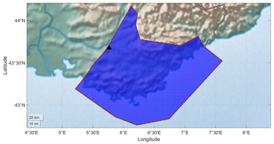
Figure 2.
The areal source used for the example hazard calculation is shown by the blue shaded region. The zone is discretized into approximately 21,000 1 km × 1 km grids. The site location is shown by the black triangle
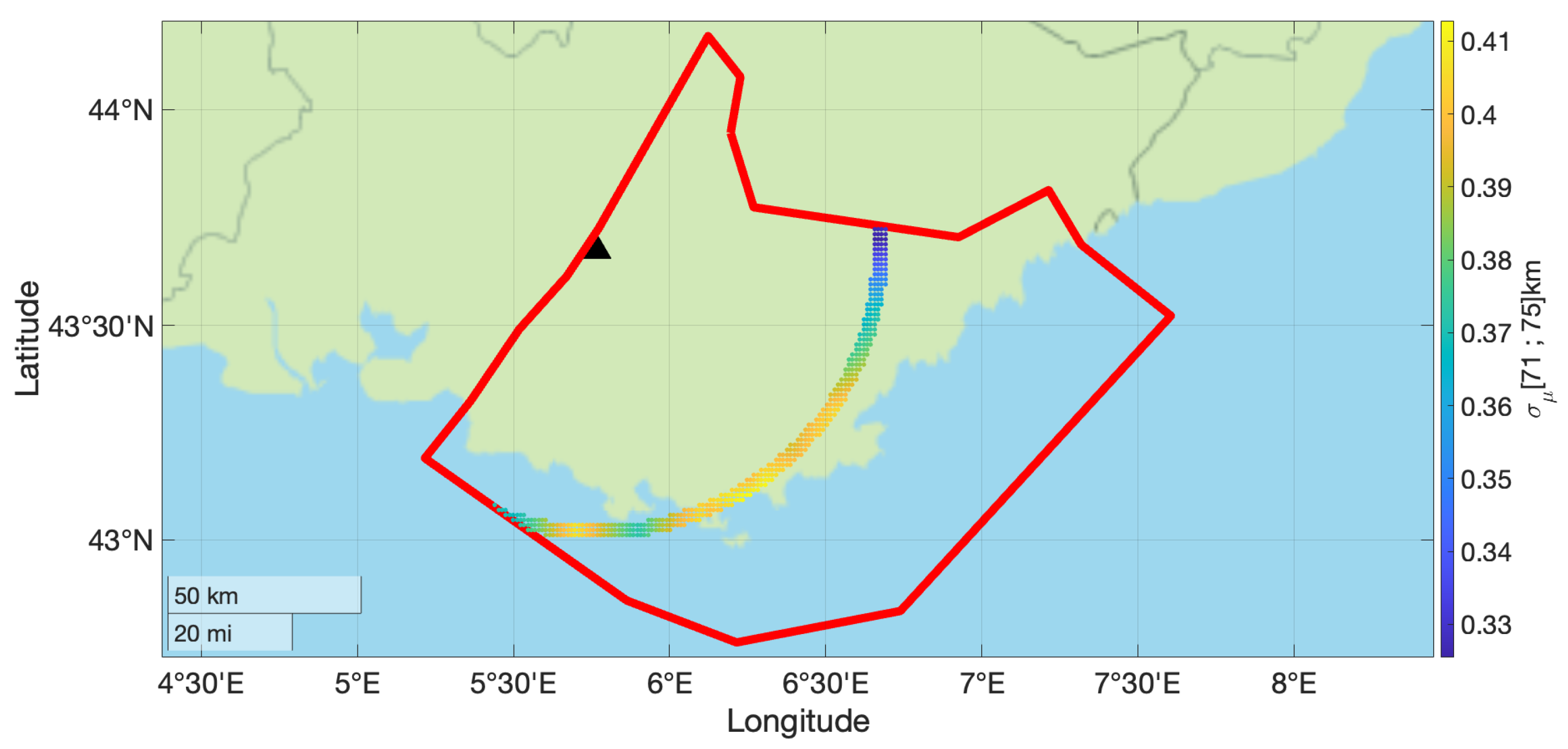
The contours of the mean and values for subsources falling in the 71–75 km distance bin are shown in Figure 3 and Figure 4. This distance bin was chosen to illustrate the proposed approach with a significant amount of seismic sources and with a broad range of non-ergodic median adjustment terms and epistemic uncertainty. The values in this distance bin range from −0.15 to 0.1 LN units.
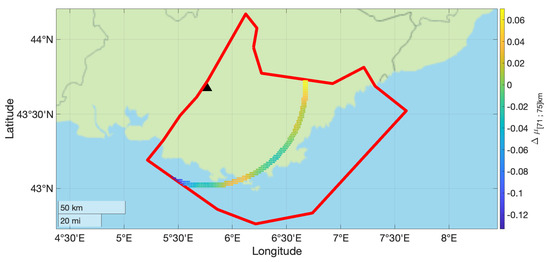
Figure 3.
Non-ergodic median adjustment terms for the subset of source locations with rupture distances between 71 km and 75 km from the site (black triangle). The red line shows the boundary of the areal source zone.

Figure 4.
Epistemic uncertainty in the non-ergodic median adjustment terms for the subset of source locations with rupture distances between 71 km and 75 km from the site (black triangle). The red line shows the boundary of the areal source zone.
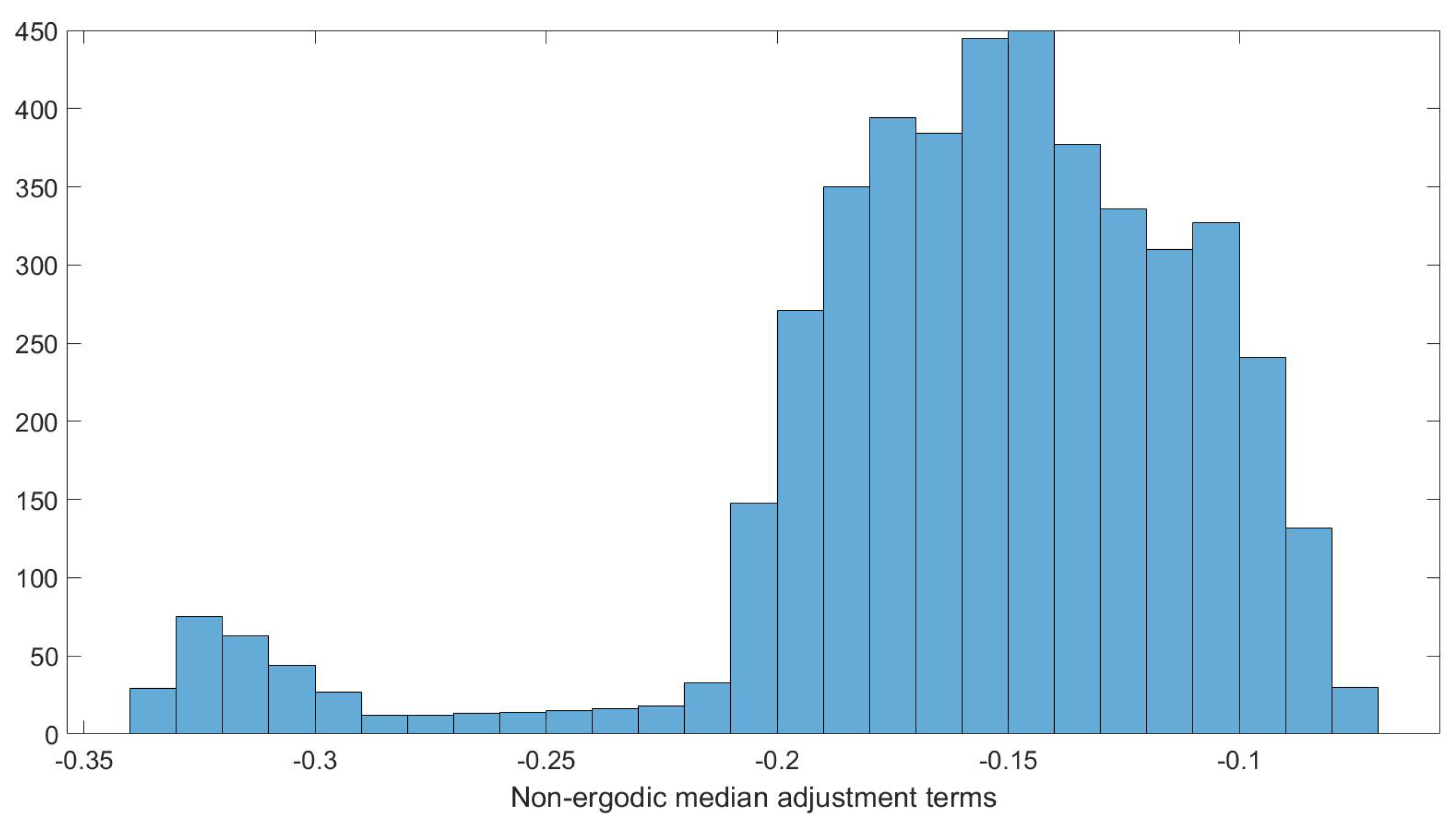
The histogram of the non-ergodic median adjustment terms, , for this distance bin is shown in Figure 5. The shape of the distribution of the terms is not close to a normal distribution, which confirms that the normal assumption is not a reasonable assumption for characterizing the distribution of the for the hazard calculation. This prevents using the PC method to estimate the hazard due to the range of within a distance bin with a single PC expansion for the distance bin.

Figure 5.
Histogram of the non-ergodic median adjustment terms between 71 km and 75 km from the site.
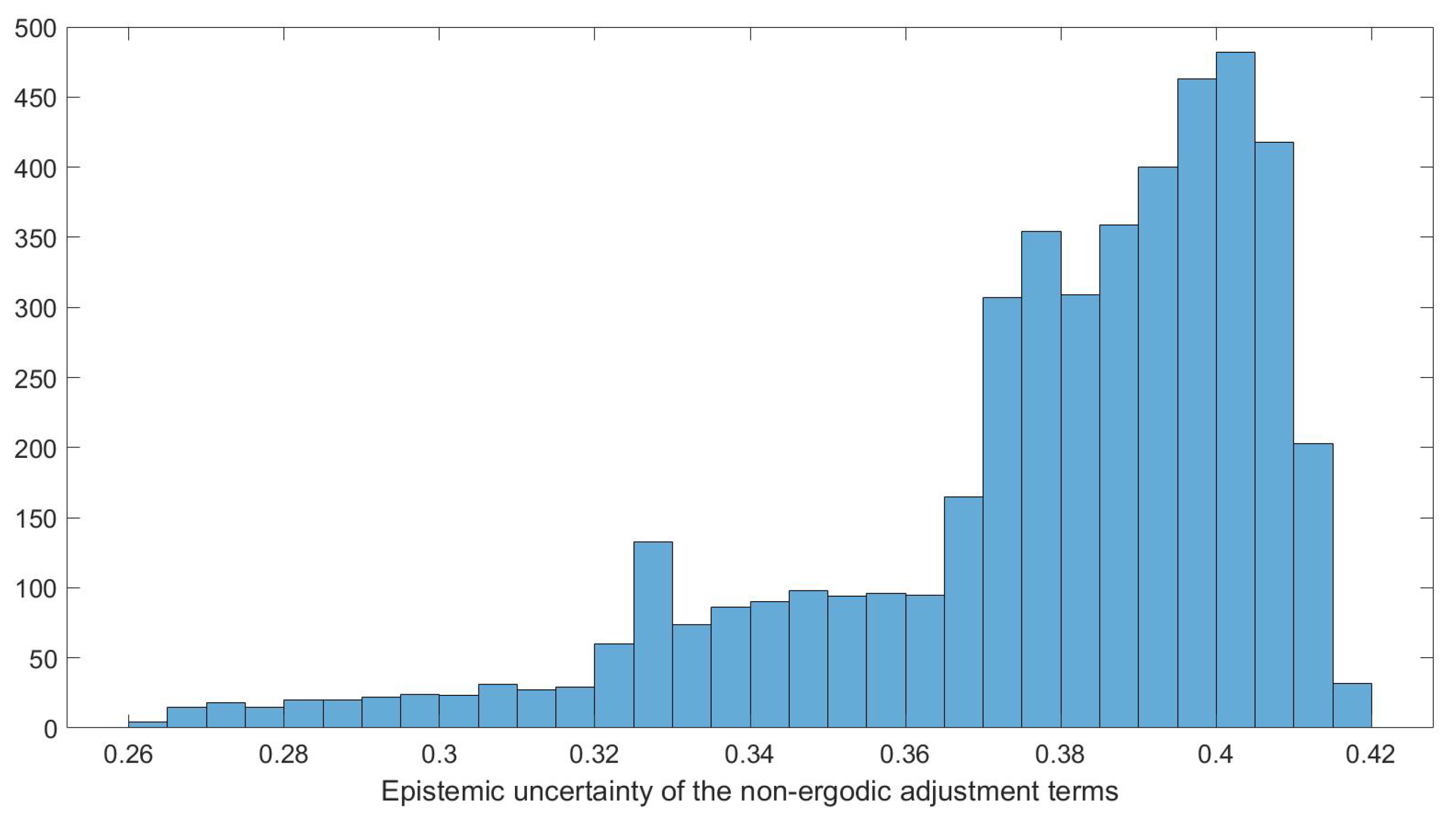
The histogram of the standard deviation of the epistemic uncertainty of the within the 71–75 km distance bin is shown in Figure 6. The distribution of the epistemic uncertainty for the sources in this distance bin is also not close to a normal distribution.

Figure 6.
Histogram of the epistemic uncertainty of the non-ergodic median adjustment terms between 71 km and 75 km from the site.
For this example, three methods are used to calculate the total hazard from the areal source under the non-ergodic assumption, including the epistemic uncertainty in the median adjustment terms: the logic tree method, the PC method, and the Taylor expansion method.
For the logic tree method, 100 samples of the spatially correlated are generated. The hazard is computed for each of the 21,000 subsources for each of the 100 samples of the .
For the PC method, five PC terms (PC order 4) are calculated for each of the 210,000 seismic sources, which results in the calculation of about 100,000 PC terms to obtain the PC expansion of the total hazard. The 100 samples of the Hermite polynomials are then generated for all the subsources. The samples are then multiplied with the PC terms of each seismic source and summed up to obtain 100 samples of the total hazard.
For the Taylor Expansion method, five PC terms are developed for the reference hazard curves, and the Taylor Expansion coefficients of order 2 are calculated for each of the 62 distance bins, resulting in the calculation of PC/TE terms. The PC terms of the seismic sources inside each distance bin are then approximated using the Taylor Expansion of the reference PC terms. For the spatially correlated case, we chose to retain 95% accuracy in the representation of the correlation structure, which led to 28 eigenfunctions retained in Equation (22). The 100 samples of the Hermite polynomials are then generated for the locations of the subsources. These samples are then multiplied with the Taylor Expansion approximation of the PC terms for each distance bin and summed up to obtain 100 samples of the total hazard.
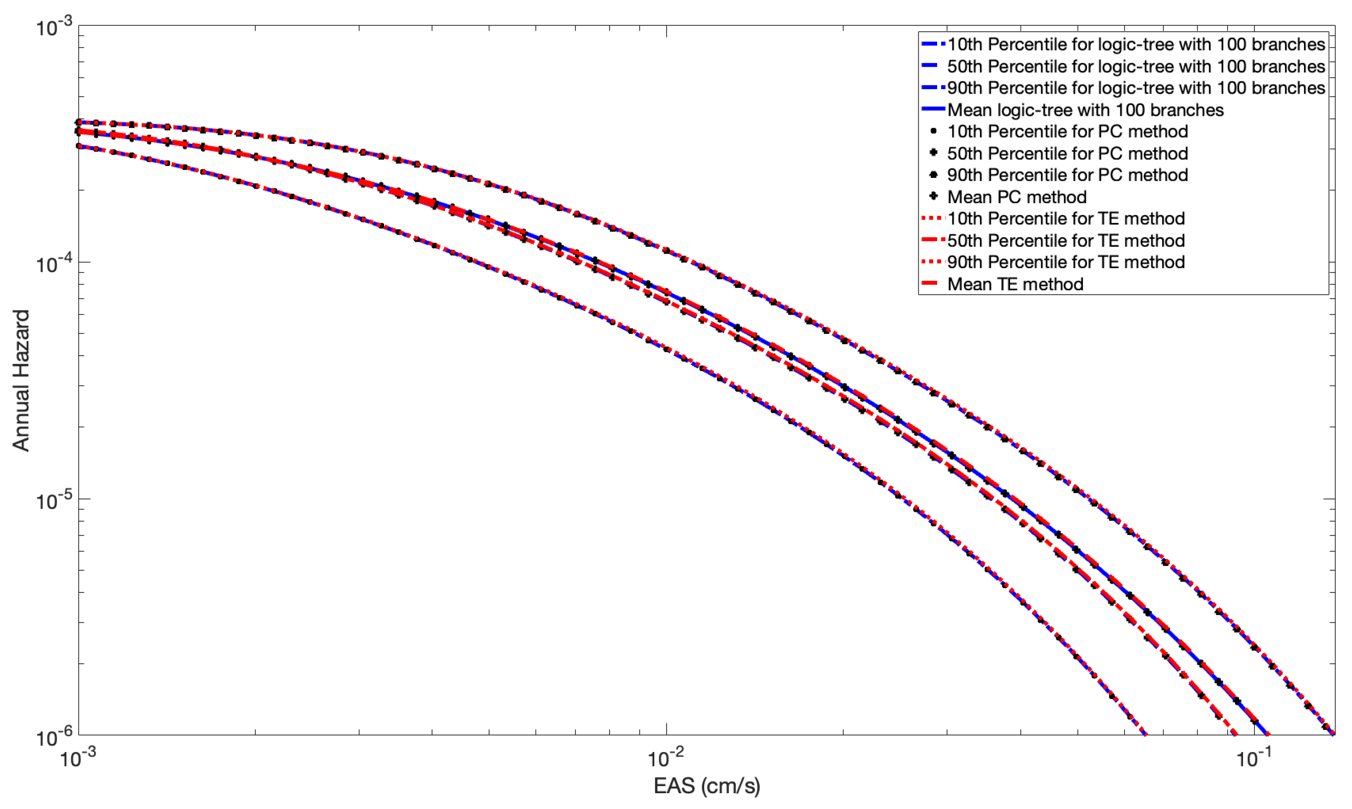
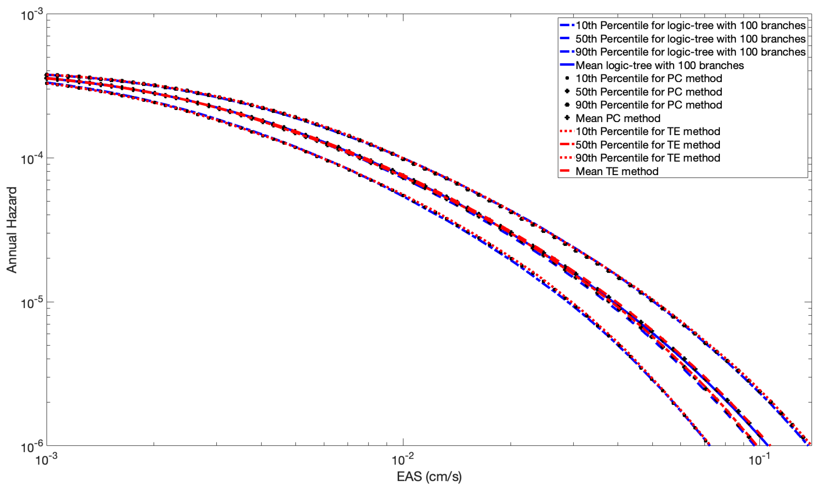
We show the percentiles of the total hazard from the three methods (Monte-Carlo (MC), Polynomial Chaos (PC) and Taylor Expansion (TE)) in Figure 7 and Figure 8 for the case of full and partial spatial correlation, respectively. The results from all three methods are very similar, indicating that the approximation used in the more efficient Taylor Expansion method has only a small reduction in accuracy.
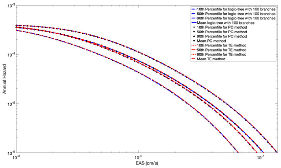
Figure 7.
Percentiles of the probability of exceedance for M = 6 with the PC method, the Taylor expansion method, and the logic tree approach (100 Branches) with full spatial correlation.
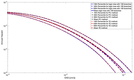
Figure 8.
Percentiles of the probability of exceedance for M = 6 with the PC method, the Taylor expansion method, and the logic tree approach (100 Branches) with partial spatial correlation.
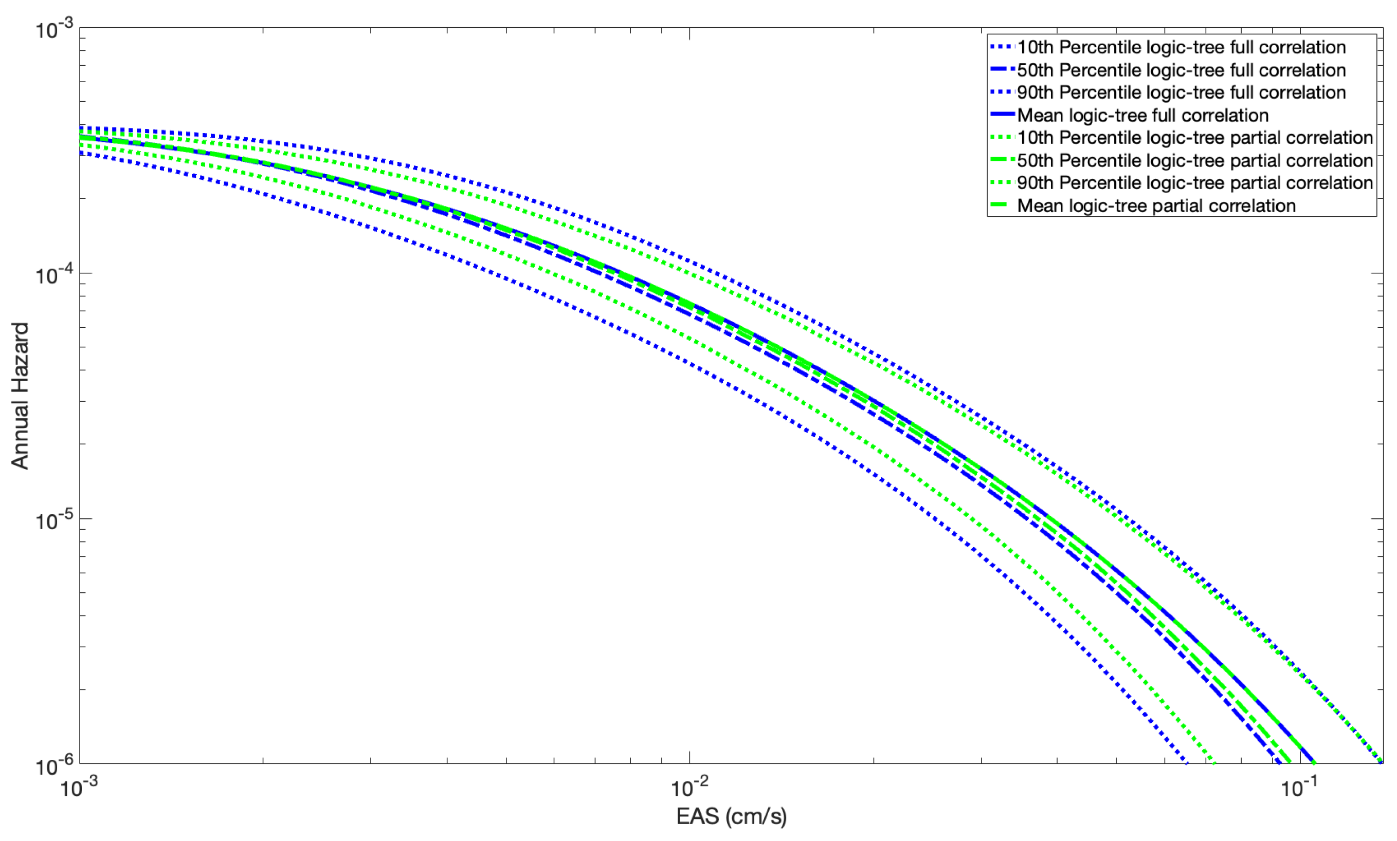
The fractiles of the total hazard with the logic tree method for the fully and partially correlated cases are shown in Figure 9. Compared to the fully correlated case, the partially correlated case gives the same mean hazard but has the effect of reducing the tails of the epistemic fractiles of the total hazard. The effect of the correlation between median ground-motion models on the total hazard was also recently investigated in [31]. The mean hazard remains identical because the mean of the samples of the median ground motion remains the same at each seismic source location in both cases; however, the spatial correlation does not allow samples of the median ground motion to have the same deviation from their mean at all seismic source locations, which reduces the number of extreme realizations of the total hazard, and therefore, reduces the tails of the hazard’s distribution.

Figure 9.
Percentiles of the probability of exceedance for M = 6 with the logic tree approach (100 Branches) with full and partial spatial correlation.
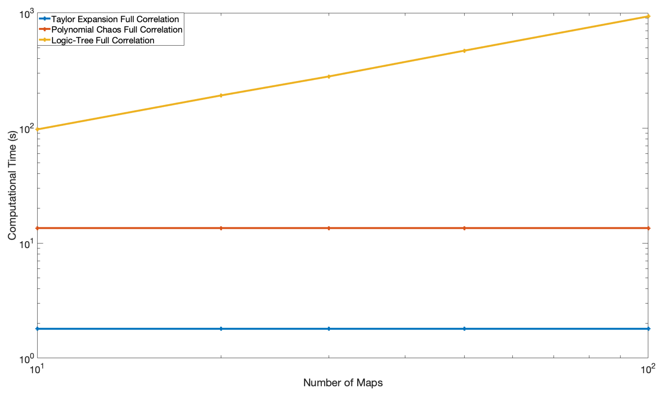
The computational time for the example hazard calculation for the logic tree, PC, and TE methods are shown in Figure 10 and Figure 11 as a function of the number of branches of the logic tree for the fully and partially correlated cases, respectively. The hazard calculation is based on a single magnitude, single source model, and single reference ergodic GMM. For the fully correlated case, the same samples of the median ground motion are used for all the seismic sources. The sampling of the hazard curves for the PC and TE methods can be performed outside of the hazard calculation in a post-processing phase. Therefore, the computational times for the PC and TE methods do not depend on the number of samples generated.
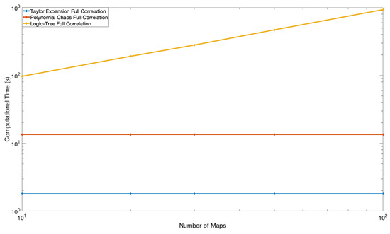
Figure 10.
Computational Time of the logic tree, Polynomial Chaos and Taylor Expansion Approaches for the Fully Correlated Cases. The x-axis is the number of branches of the on the logic tree.
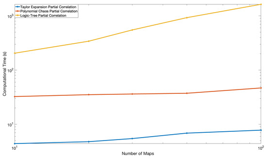
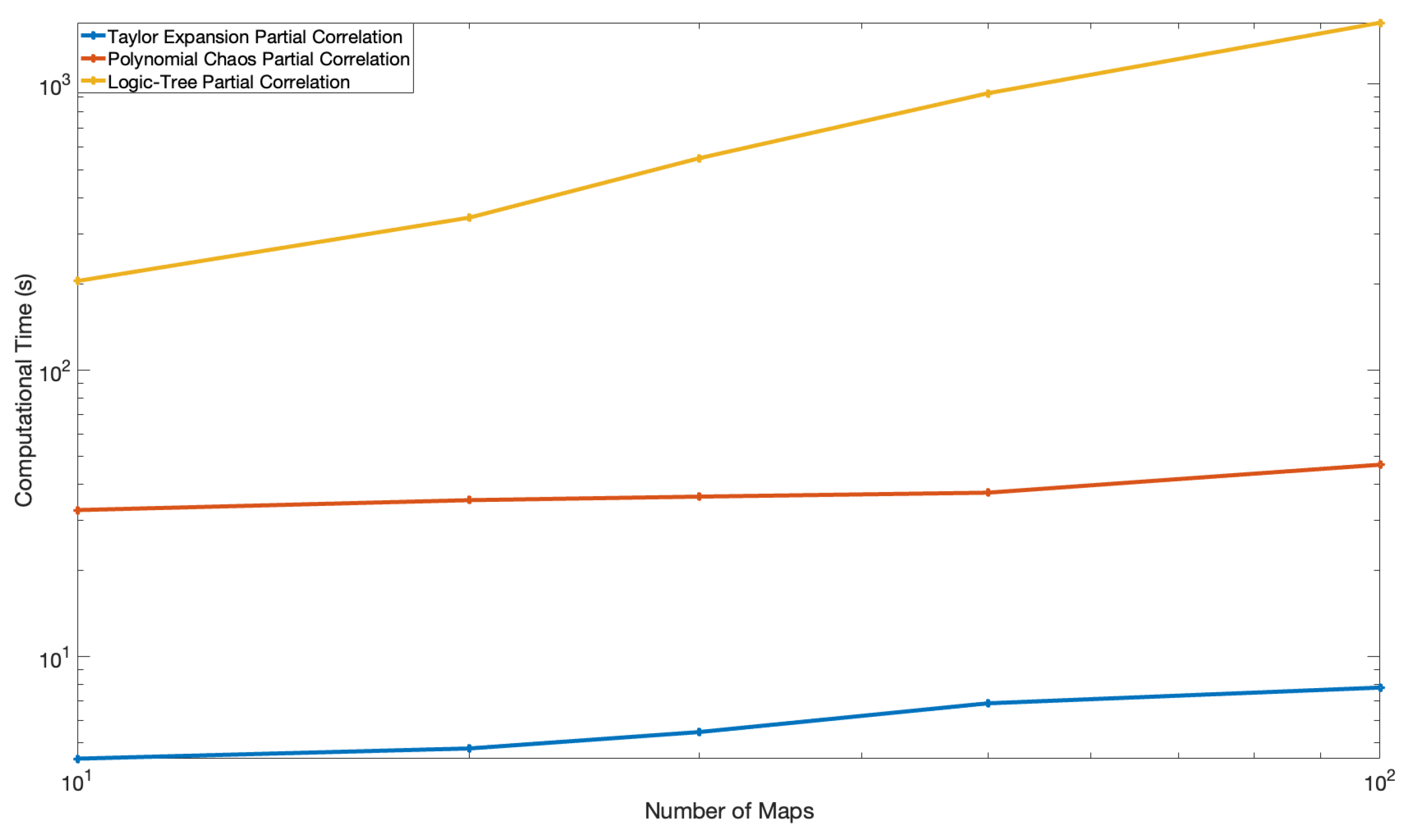
Figure 11.
Computational Time of the logic tree, Polynomial Chaos and Taylor Expansion Approaches for the Partially Correlated Cases. The x-axis is the number of branches of the on the logic tree.
For the partially correlated case, the computational time depends on the number of samples generated for the three methods, and they all scale linearly with the number of median ground-motion samples; however, the PC method remains significantly faster by several orders of magnitude compared to the logic tree method, and the TE method performs one order of magnitude faster than the PC method for an equal number of samples generated.
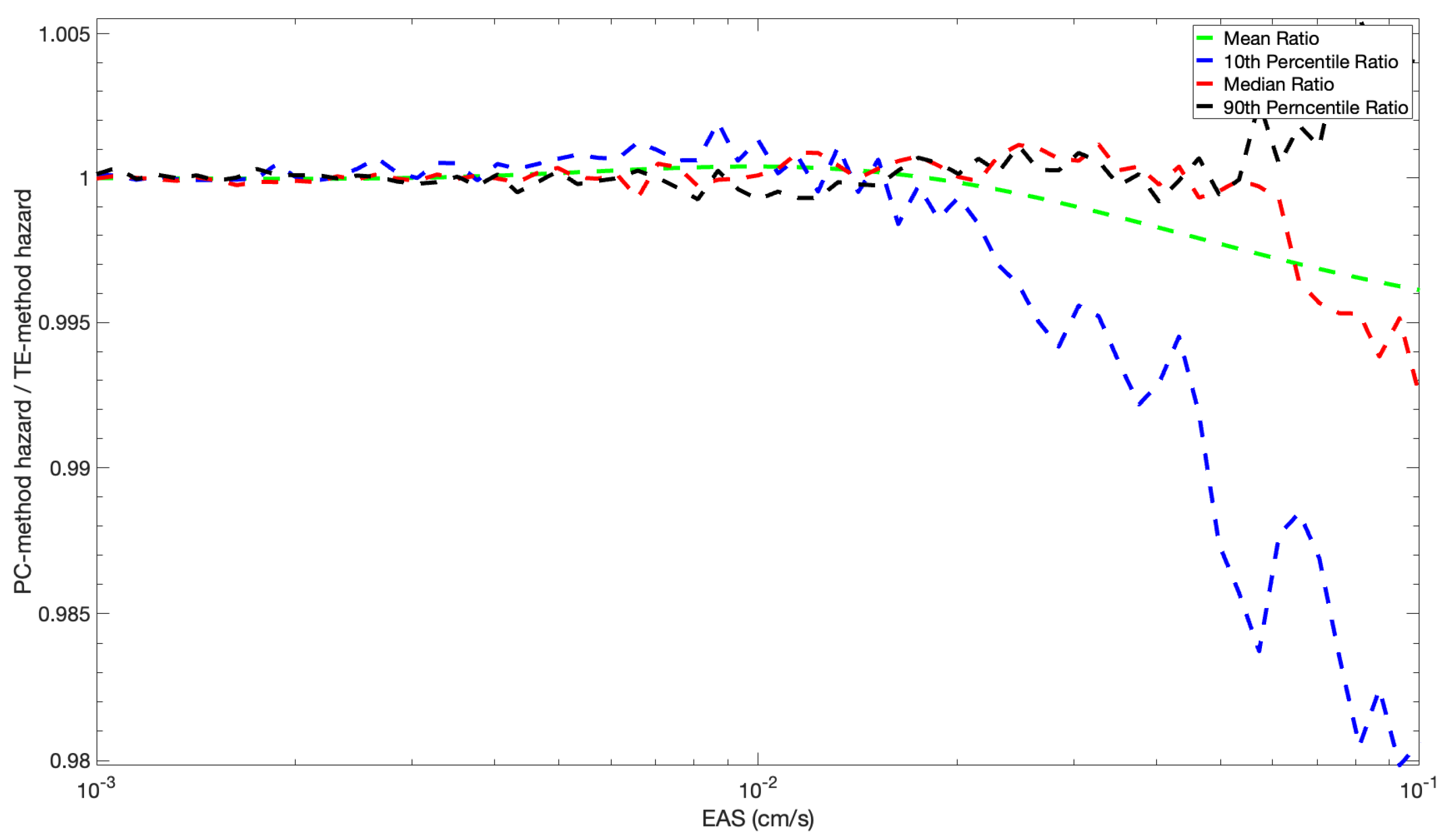
The accuracy of the mean hazard and hazard fractiles for the TE method for the example is shown in Figure 12. At the higher ground-motion values, the hazard (y-axis value) for the TE method is about 2% larger than for the PC method. This is smaller than the difference in the hazard found using different hazard programs. In this example, the error is due to the TE approximation of the PC coefficient, which can be reduced by increasing the order of the TE expansion (a TE expansion of order 2 was chosen here).

Figure 12.
Ratio of Fractiles of the Annual Hazard of the PC Method by the Taylor Expansion Method.
5. Conclusions
Advances in ground-motion models are leading to larger and more complex logic trees. In particular, the move to non-ergodic GMMs leads to an additional node on the logic tree to capture the epistemic uncertainty of the non-ergodic terms. To include the spatial correlation of the non-ergodic terms as part of the logic tree branches, a large number of branches (e.g., 100) are included, which greatly increases the calculation time. As the calculation time becomes an issue, more of the effort for a PSHA goes into managing the long calculation times, leaving less time for sensitivity studies to better understand the effects of different models and parameters on the hazard.
To reduce the computational burden for non-ergodic hazard calculations for areal seismic sources, the PC method [30] together with a Taylor expansion of the PC terms can be used to efficiently and accurately compute the mean hazard and epistemic fractiles of the hazard. For a logic tree with 100 branches for the alternative models for the non-ergodic terms, the proposed method reduces the hazard calculation time by a factor of 50 to 100. This gain of computational speed will be valuable for non-ergodic hazard calculations with areal sources and allow for more time to be spent on gaining a better understanding of the hazard and less time on completing the hazard calculations.
While this paper focused on the analytical approximations of the hazard for non-ergodic GMMs, the analytical approximations of the hazard can also be used for other nodes of the logic tree. Approximate methods that sample the full epistemic uncertainty distribution can lead to more accurate estimates of the epistemic fractiles of the hazard than using crude sampling of the epistemic uncertainty distribution with an exact hazard calculation for each branch of the logic tree.
The results of this study can be used by developers of PSHA software to implement GMMs with non-ergodic path effects into their software. Other researchers can use this type of approach to develop analytical approximations for propagating the epistemic uncertainty for other nodes of the logic tree as more complex models, such as non-Poisson earthquake occurrence, are incorporated into the hazard calculation.
Supplementary Materials
The following supporting information can be downloaded at: https://www.mdpi.com/article/10.3390/app15052454/s1
Author Contributions
Conceptualization, N.A. and M.L.; methodology, M.L.; application, M.L.; writing—original draft preparation, M.L.; writing—review and editing, N.A. All authors have read and agreed to the published version of the manuscript.
Funding
This research received no external funding.
Institutional Review Board Statement
Not applicable.
Informed Consent Statement
Not applicable.
Data Availability Statement
The data for the maps of the non-ergodic terms used in the example hazard calculation are available at https://github.com/abrahamson/Lacour_abrahamson_2025_. This was last accessed 24 February 2025. No new data were generated during the study.
Acknowledgments
Overleaf v5.3.1 and Grammarly v9.75.0 were used for preparing the article and checking the spelling and grammar.
Conflicts of Interest
The authors declare no conflicts of interest.
References
- Committee, S.S.H.A. Recommendations for 48 Probabilistic Seismic Hazard Analysis—Guidance on Uncertainty and Use of Experts; Technical Report; U.S. Nuclear Regulatory Commission: Rockville, MA, USA, 1997.
- Chiou, B.S.J.; Youngs, R.R. Update of the Chiou and Youngs NGA model for the average horizontal component of peak ground motion and response spectra. Earthq. Spectra 2014, 30, 1117–1153. [Google Scholar] [CrossRef]
- Anderson, J.G.; Brune, J.N. Pobabilistic seismic hazard analysis without the ergodic assumption. Bull. Seismol. Soc. Am. 1999, 96, 446–455. [Google Scholar]
- Graves, R.; Pitarka, A.; Somerviell, P. Ground motion amplification in the Santa Monica area: Effects of shallow basin edge structure. Bull. Seismol. Soc. Am. 1998, 88, 1224–1242. [Google Scholar] [CrossRef]
- Kawase, H. The cause of the damage belt in Kobe: ‘The basin edgeeffect’, constructive interference of the direct S-wave with the basin induced diffracted/Rayleigh waves. Seismol. Res. Lett. 1996, 67, 25–34. [Google Scholar] [CrossRef]
- Kohler, M.D.; Filippitzis, F.; Heaton, T.; Clayton, R.; Guy, R.; Bunn, J.; Chandy, K. 2019 Ridgecrest earthquake reveals areas of Los Angeles that amplify shaking of high-rises. Seismol. Res. Lett. 2020, 91, 3370–3380. [Google Scholar] [CrossRef]
- Atkinson, G.M. Single-station sigma. Bull. Seismol. Soc. Am. 2006, 96, 446–455. [Google Scholar] [CrossRef]
- Rodriguez-Marek, A.; Montalva, G.; Cotton, F.; Bonilla, F. Analysis of single-station standard deviation using the KiK-net data. Bull. Seismol. Soc. Am. 2011, 101, 1242–1258. [Google Scholar] [CrossRef]
- Lanzano, G.; D’Amico, M.; Felicetta, C.; Luzi, L.; Puglia, R. Update of the single-station sigma analysis for the Italian strong-motion stations. Bull. Earthq. Eng. 2017, 15, 2411–2428. [Google Scholar] [CrossRef]
- Sung, C.H.; Lee, C.T. Improvement of the Quantification of Epistemic Uncertainty Using Single-Station Ground-Motion Prediction Equations. Bull. Seismol. Soc. Am. 2019, 109, 1358–1377. [Google Scholar] [CrossRef]
- Morikawa, N.; Kanno, T.; Narita, A.; Fujiwara, H.; Okumura, T.; Fukushima, Y.; Guerpinar, A. Strong motion uncertainty determined from observed records by dense network in Japan. J. Seismol. 2008, 12, 529–546. [Google Scholar] [CrossRef]
- Anderson, J.G.; Uchiyama, Y. A methodology to improve ground-motion prediction equations by including path corrections. Bull. Seismol. Soc. Am. 2011, 101, 1822–1846. [Google Scholar] [CrossRef]
- Parker, G.; Baltay, A. Empirical Map-Based Nonergodic Models of Site Response in the Greater Los Angeles Area. Bull. Seismol. Soc. Am. 2022, 122, 1607–1629. [Google Scholar] [CrossRef]
- Dawood, H.; Rodriguez-Marek, A. A method for including path effects in ground-motion prediction equations: An example using the Mw 9.0 Tohoku earthquake aftershocks. Bull. Seismol. Soc. Am. 2013, 103, 1360–1372. [Google Scholar] [CrossRef]
- Sung, C.H.; Lee, C.T. A new methodology for quantification of the systematic path effects on ground-motion variability. Bull. Seismol. Soc. Am. 2016, 106, 2796–2810. [Google Scholar] [CrossRef]
- Graves, R.; Jordan, T.H.; Callaghan, S.; Deelman, E.; Field, E.; Juve, G.; Kesselman, C.; Maechling, P.; Mehta, G.; Milner, K.; et al. CyberShake: A physics-based seismic hazard model for southern California. Pure Appl. Geophys. 2011, 168, 367–381. [Google Scholar] [CrossRef]
- Wang, F.; Jordan, T.H. Comparison of probabilistic seismic-hazard models using averaging-based factorization. Bull. Seismol. Soc. Am. 2014, 104, 1230–1257. [Google Scholar] [CrossRef]
- Meng, X.; Goulet, C.; Milner, K.; Graves, R.; Callaghan, S. Comparison of Nonergodic Ground-Motion Components from CyberShake and NGA-West2 Datasets in California. Bull. Seismol. Soc. Am. 2023, 113, 1152–1175. [Google Scholar] [CrossRef]
- Maeda, T.; Iwaki, A.; Morikawa, N.; Aoi, S.; Fujiwar, H. Seismic-hazard analysis of long-period ground motion of megathrust earthquakes in the Nankai trough based on 3D finite difference simulation. Seismol. Res. Lett. 2016, 87, 1265–1273. [Google Scholar] [CrossRef]
- Moschetti, M.; Hartzell, S.; Ramírez-Guzman, L.; Frankel, A.; Angster, S.; Stephenson, W. 3D ground-motion simulations of Mw 7 earthquakes on the Salt Lake City segment of the Wasatch Fault zone: Variability of long-period (T gt 1 s) ground motions and sensitivity to kinematic rupture parameters. Bull. Seismol. Soc. Am. 2017, 107, 1704–1723. [Google Scholar]
- Frankel, A.; Wirth, E.; Marafi, N.; Vidale, J.; Stephenson, W. Broadband synthetic seismograms for magnitude 9 earthquakes on the Cascadia megathrust based on 3D simulations and stochastic synthetics, Part 1: Methodology and overall results. Bull. Seismol. Soc. Am. 2018, 108, 2347–2369. [Google Scholar] [CrossRef]
- Stewart, J.P.; Afshari, K.; Goulet, C.A. Non-Ergodic Site Response in Seismic Hazard Analysis. Earthq. Spectra 2017, 33, 1385–1414. [Google Scholar] [CrossRef]
- Bommer, J.J.; Coppersmith, K.J.; Coppersmith, R.T.; Hanson, K.L.; Mangongolo, A.; Neveling, J.; Rathje, E.M.; Rodriguez-Marek, A.; Scherbaum, F.; Shelembe, R.; et al. A SSHAC level 3 probabilistic seismic hazard analysis for a new-build nuclear site in South Africa. Earthq. Spectra 2015, 31, 661–698. [Google Scholar] [CrossRef]
- Coppersmith, K.; Bommer, J.; Hanson, K.; Unruh, J.; Coppersmith, R.; Wolf, L.; Youngs, R.; Rodriguez-Marek, A.; Al Atik, L.; Toro, G.; et al. Hanford Sitewide Probabilistic Seismic Hazard Analysis; Technical Report Report Number: PNNL-23361; Pacific Northwest National Laboratory: Richland, WA, USA, 2014. [Google Scholar]
- GeoPentech. Southwestern United States Ground Motion Characterization SSHAC Level 3; Technical Report Technical Report, rev. 2; Pacific Gas and Electric Company: San Francisco, CA, USA, 2015. [Google Scholar]
- Kotha, S.R.; Bindi, D.; Cotton, F. Partially non-ergodic region specific GMPE for Europe and Middle-East. Bull. Earthq. Eng. 2016, 14, 1245–1263. [Google Scholar] [CrossRef]
- Bommer, J.; Scherbaum, F. The use and misuse of logic trees in probabilistic seismic hazard analysis. Earthq. Spectra 2008, 24, 997–1009. [Google Scholar] [CrossRef]
- McGuire, R.K. Seismic Hazard and Risk Analysis; Earthquake Engineering Research Institute: Oakland, CA, USA, 2004. [Google Scholar]
- Baker, J.; Bradley, B.; Stafford, P. Seismic Hazard and Risk Analysis; Cambridge University Press: Cambridge, UK, 2021. [Google Scholar]
- Lacour, M.; Abrahamson, N. Efficient Propagation of Epistemic Uncertainty in the Median Ground-Motion Model in Probabilistic Hazard Calculations. Bull. Seismol. Soc. Am. 2019, 109, 2063–2072. [Google Scholar] [CrossRef]
- Lacour, M.; Abrahamson, N. Efficient Propagation of Epistemic Uncertainty for Probabilistic Seismic Hazard Analyses (PSHAs) Including Partial Correlation of Magnitude–Distance Scaling. Bull. Seismol. Soc. Am. 2021, 110, 3332–3340. [Google Scholar] [CrossRef]
- Halko, N.; Martinsson, P.; Tropp, J. Finding Structure with Randomness: Probabilistic Algorithms for Constructing Approximate Matrix Decompositions. SIAM Rev. 2011, 53, 217–288. [Google Scholar] [CrossRef]


Disclaimer/Publisher’s Note: The statements, opinions and data contained in all publications are solely those of the individual author(s) and contributor(s) and not of MDPI and/or the editor(s). MDPI and/or the editor(s) disclaim responsibility for any injury to people or property resulting from any ideas, methods, instructions or products referred to in the content. |
© 2025 by the authors. Licensee MDPI, Basel, Switzerland. This article is an open access article distributed under the terms and conditions of the Creative Commons Attribution (CC BY) license (https://creativecommons.org/licenses/by/4.0/).