Impact of Twisting on Skin and Proximity Losses in Segmented Underground Cables: A 3D Finite-Element Study

Abstract

This paper presents a comprehensive three-dimensional (3D) finite-element (FE) study of skin and proximity losses in a five-segment, helically twisted underground power cable. Unlike conventional two-dimensional (2D) analyses—which assume parallel conductors and consequently overestimate eddy current losses—our 3D approach accurately captures the effects of varying lay lengths ($\lambda$). Simulations are performed from 0 Hz (DC) to 50 Hz, showing that while the per-unit-length DC resistance remains unaffected by twisting, the AC resistance can increase significantly depending on the pitch. At 50 Hz, the ratio of AC to DC resistance ($R_{\mathrm{AC}}$/$R_{\mathrm{DC}}$) ranges from about 1.32 for very tight twists ($\lambda =0.1\mathrm{m}$) to nearly 1.72 for gentle pitches ($\lambda =5.0\mathrm{m}$). Further analysis reveals that short lay lengths enhance magnetic field coupling, improving current distribution and partially mitigating losses. To quantify these findings, an exponential-saturation model is proposed to describe $R_{\mathrm{AC}}$/$R_{\mathrm{DC}}$ as a function of lay length, achieving excellent agreement ($R^2\approx 0.996$) with the 3D FE data. These results underscore the importance of considering full 3D geometry in cable design, offering a practical tool for optimizing both mechanical reliability and electromagnetic performance in high-voltage underground applications.

1. Introduction

Twisted and stranded conductors are ubiquitous in high-voltage and extra-high-voltage (EHV) underground power cables. By helically arranging conductor segments or sub-bundles, cable manufacturers can improve mechanical robustness and mitigate certain electromagnetic imbalances [1,2]. While these benefits are well recognized, the electromagnetic implications of twisting—particularly on skin and proximity losses—are also significant. Under alternating-current (AC) conditions, twisting modifies both the skin and proximity effects [3,4], which, in turn, affect the AC resistance and power dissipation of the cable.

Several studies on twisted conductors provide important background for the present work. For example, ref. [5] investigated the influence of inner skin- and proximity effects on conduction in Litz wires using three-dimensional finite-element (3D-FE) simulations, highlighting the critical role of twisting in current redistribution. Ref. [6] further analyzed loss mechanisms in multistranded twisted wires via 3D-FE simulations, demonstrating that twisting not only affects the strand-level eddy currents but also introduces additional bundle-level losses. In high-speed permanent magnet machines, ref. [7] showed that transposition of insulated strands can reduce bundle proximity losses, emphasizing the sensitivity of loss mechanisms to the twisting configuration. Complementary analytical approaches have also been developed, ref. [8] formulated a complete analytical model to capture the effects of twisting on Litz-wire losses, while [9] provided a 3D finite-element simulation of Litz wires with multilevel bundle structures that captures the complexity of the twisting operations. Finally, ref. [10] exploited helicoid symmetry to reduce the dimensionality of eddy-current problems in power cables, offering further insights into the impact of twisting on conductor performance.

While DC resistance ($R_{\mathrm{DC}}$) grows with length, AC resistance ($R_{\mathrm{AC}}$) also includes frequency-dependent skin and proximity effects [11,12]. In multi-segment cables, twisting reorients segments along z, altering how eddy currents form near segment boundaries. Consequently, $R_{\mathrm{AC}}$ is not solely a function of length but also the electromagnetic coupling among segments. Thus, shorter lay lengths can yield different $R_{\mathrm{AC}}/R_{\mathrm{DC}}$ values than more gently twisted cables. Unlike previous two-dimensional (2D) analyses that approximate sub-conductors as parallel elements [13,14], the present study employs a comprehensive 3D FE approach that explicitly accounts for the helical geometry.

This paper focuses on a five-segment underground cable design, where each segment is treated as a solid bundle of hexagonally packed copper strands. Fourteen distinct 3D models are constructed, each one completing exactly one full 360° rotation around the cable’s central axis with a different lay length $\lambda$ (0.1 m to 5.0 m). Simulations performed from 0 Hz (DC) to 50 Hz reveal that while the per-unit-length DC resistance remains constant with twisting, the AC resistance changes significantly with varying lay length. Specifically, at 50 Hz, the ratio $R_{\mathrm{AC}}/R_{\mathrm{DC}}$ ranges from about 1.32 for very tight twists (lay length $\lambda =0.1\mathrm{m}$) to nearly 1.72 for gentle twists ($\lambda =5.0\mathrm{m}$). An exponential-saturation model is proposed to describe this trend, yielding excellent agreement ($R^2\approx 0.996$) with the 3D FE data. These findings underscore the importance of accurately capturing 3D twisting effects not only for loss prediction but also for optimizing both mechanical and electromagnetic performance in high-voltage underground cable designs. The paper also discusses mesh design, numerical errors, and a general method to incorporate effective conductor length changes due to twisting. The present work thus addresses the key research questions:

• How does twisting angle (or lay length) affect ${\mathrm{R}}_{\mathrm{AC}}/{\mathrm{R}}_{\mathrm{DC}}$ for multi-segment cables under typical operating frequencies?
• What is the relative difference in AC losses between very short (tightly twisted) and large (nearly parallel) lay lengths?
• Can an analytical or semi-empirical model describe the ${\mathrm{R}}_{\mathrm{AC}}/{\mathrm{R}}_{\mathrm{DC}}$ trend as a function of lay length?

The remainder of the paper is organized as follows. Section 2 introduces the twisted cable model and the effective length concept. Section 3 describes the 3D finite-element approach, while Section 4 presents 2D benchmark cases. Section 5 details the numerical results and the exponential-saturation model for $R_{\mathrm{AC}}/R_{\mathrm{DC}}$ versus lay length. Finally, Section 6 summarizes the key insights and outlines future directions.

2. Cable Model and Effective Length in 3D Twisted Conductors

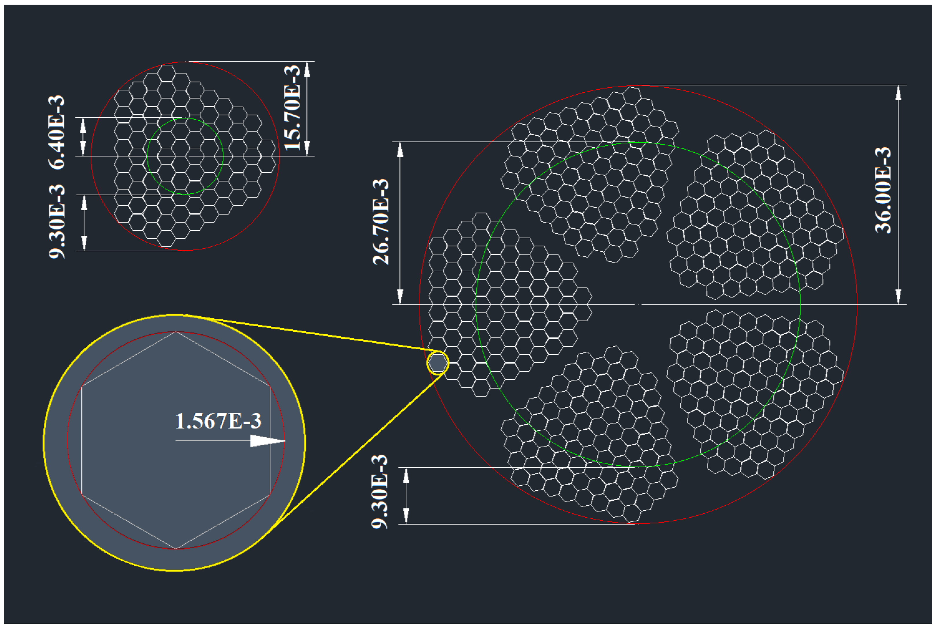
2.1. Overview of the Baseline Cable

A five-segment cable configuration, based on a previous work by [15], is established by subdividing a large conductor cross-section (≈$2711{\mathrm{mm}}^2$ total) into five bundles, each containing 85 hexagonally packed (under full compression assumption) conductor strands with no electrical insulation between the strands in each bundle, and therefore, each segment can be treated as a solid bundle from a perspective of electromagnetic behaviour. Figure 1 illustrates detailed schematic of the cable’s cross-section with all measurements in meter. The outer air boundary extends $30\mathrm{cm}$ radially from the cable’s center for all models in this study. In the parallel (untwisted) scenario, the cable is extruded along the z-axis with no helical pitch, effectively forming a purely longitudinal arrangement of sub-conductors.

The 3D parallel model extends $4\mathrm{m}$ in the longitudinal direction, capturing the same cross-section along its entire length (see Figure 2). Under AC current, the skin and proximity effects within each bundle drive the current toward the outer periphery and near inter-bundle boundaries.

2.2. Introducing Twisting: Lay Length Definition

In practical cable designs, the five segments often twist around the central axis to improve mechanical stability and reduce certain electromagnetic imbalances. Twisting is typically parameterized by a lay length $\lambda$, defined as the longitudinal distance required for one full ${360}^{\circ }$ twist [16,17]. A smaller $\lambda$ implies a tighter pitch (more twists per meter), while a larger $\lambda$ indicates a gentler helix, approaching a parallel arrangement as $\lambda \to \infty$.

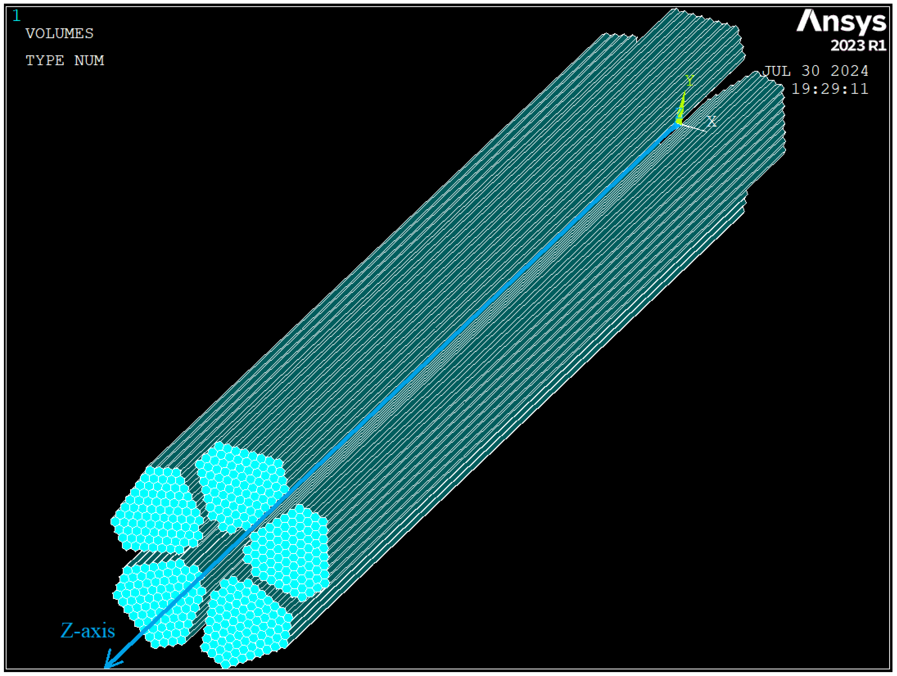
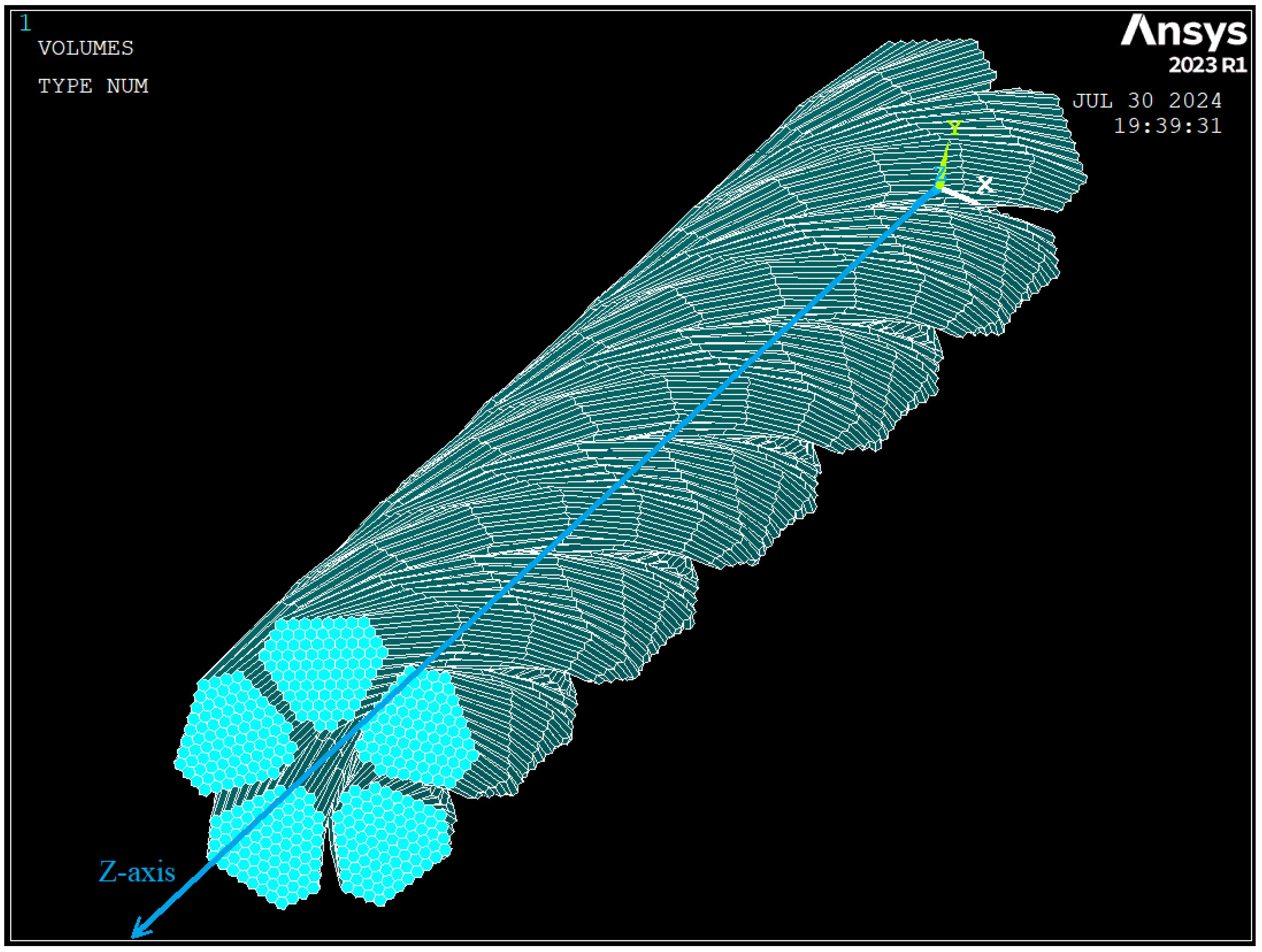
2.2.1. Helical Transformation

Figure 3 displays a conceptual 3D model for the five-segment cable with twisting. Mathematically, the center of each segment is rotated about the z-axis as a function of z as

$$\theta \left(z\right)={\displaystyle \frac{2\pi }{\lambda }}z,$$

(1)

where $\lambda$ is the specified lay length. Each segment’s cross-section is swept along this helical path to create the final cable geometry. Within each segment itself, no additional twisting of individual strands is considered (i.e., each segment is internally “solid”).

2.2.2. Range of Lay Lengths Studied

To capture a broad range of twisting scenarios, $\lambda$ is swept from $0.1\mathrm{m}$ (very tight twist) up to $5.0\mathrm{m}$ (nearly parallel). The total extruded length of each model is equal to $\lambda$. To achieve exactly one full turn over length $\lambda$, the model is parameterized such that z runs from 0 to $\lambda$, and the segment centroid is rotated ${360}^{\circ }$ about the z-axis over these interval steps. This is a complex geometry design which was achieved by changing the software’s Global Coordinate System to cylindrical when extruding the 2D areas into three-dimensional volumes alongside the z-axis and offsetting its angle by a certain degree on every step of the extrusion.

The 2D cross-sectional areas for one-fifth of the cable (Figure 4a) are first imported in IGES format. Then, by adjusting the lay length parameter in the APDL batch script (LayLength), the same 2D model is extruded and replicated at varying pitches to produce different twisted geometries. Below is an excerpt of the APDL code to create the volumes:

!------------------------------Define Parameters.

LayLength = 1

NumberOfDivisions = 16

OffSetAng = 360/NumberOfDivisions

OffSetZ = LayLength/NumberOfDivisions

!------------------------------Making the 1/5 slice volume twisted.

!--------------------Change Active CS to Cylindrical.

CSYS,1

!--------------------Do Loop - Modeling one twisted volume at a time.

/prep7

*DO,i,3,88,1

ASEL,S,,,i

VEXT,ALL,,,0,OffSetAng,OffSetZ,,,,

VGEN,NumberOfDivisions,1,,,0,OffSetAng,OffSetZ,,0

VSEL,S,,,1,NumberOfDivisions,,

VADD,ALL

*ENDDO

!------------------------------Partitioning all the conductors and the air.

ALLSEL,ALL

VPTN,ALL

!------------------------------Copy the 1/5 slice section five times.

VGEN,5,ALL,,,0,72,0,0,0

In this macro:

• LayLength sets the total helical pitch (0.1–5 m), while NumberOfDivisions controls how many increments ($\mathtt{VEXT}$ and VGEN) will be used to create the continuous twist;
• The variables OffSetAng and OffSetZ are computed, ensuring a uniform and persise helical extrusion in cylindrical coordinates;
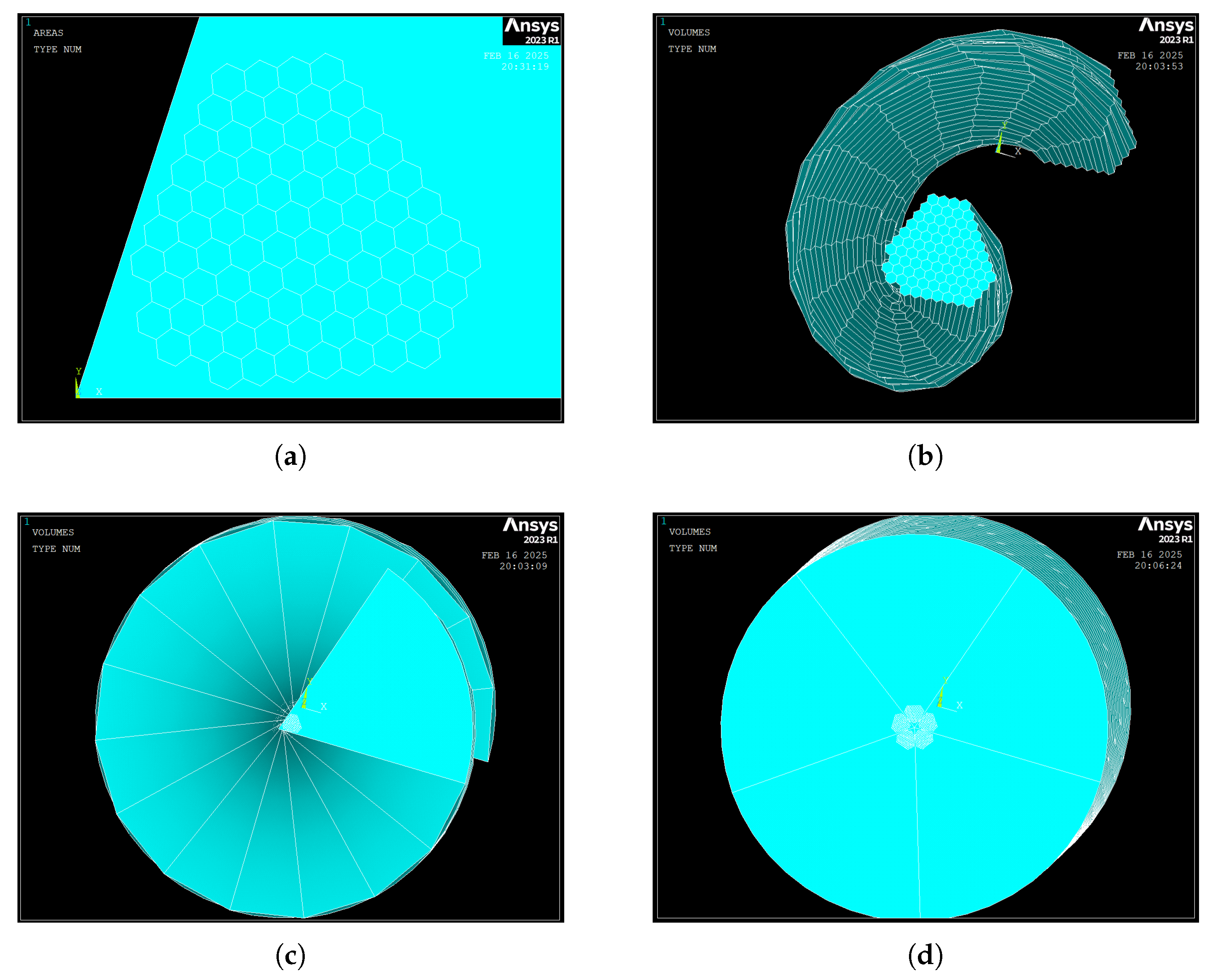
• A DO loop (from lines *DO,i,3,88,1) selects each 2D area in turn (ASEL), then extrudes (VEXT) and replicates (VGEN) the geometry with the appropriate angular and z-axis offset (Figure 4b,c);
• Once the single-fifth twist is complete, it is repeated five times (VGEN,5,ALL) to form the full 360° cross-section (Figure 4d).

By simply changing LayLength in this script (for instance, from 0.1 m to 5 m), the same input 2D areas yield different 3D twisted models. Subsequent steps—such as meshing, material property assignments, and boundary conditions—are identical for each geometry, enabling a systematic investigation of how the lay length affects AC and DC resistive losses.

2.3. The Effective Length $l_{\mathrm{twist}}$ in 3D Models

Accurate calculation of conductor resistance requires proper accounting of the true path length that current travels [1]. Unlike simplified 2D analyses (which often represent an ideal cross-section with negligible length), 3D twisted models explicitly incur a helix path for each conductor. The direct-current (DC) resistance $R_{\mathrm{DC}}$ thus depends on how much extra length is introduced by the twisting.

2.3.1. Numerical Calculation of the Effective Length $l_{\mathrm{twist}}$

Let $\lambda$ be the linear distance along the z-axis for a full turn, and r be the radial distance of a given conductor from the central axis as shown in Figure 5. Then, a single conductor’s helix length $l_{\mathrm{twist}}$ for one turn can be approximated by the Pythagorean relation:

$$l_{\mathrm{twist}}=\sqrt{{\lambda }^2+{\left(2\pi r\right)}^2}.$$

(2)

In multi-layer or multi-segment cables, r may differ among conductors. Tighter twisting (small $\lambda$) increases the ratio $l_{\mathrm{twist}}/\lambda$ more substantially, raising the DC resistance because $R_{\mathrm{DC}}\propto length$.

2.3.2. Practical Computation of the Effective Length $l_{\mathrm{twist}}$

The $l_{\mathrm{twist}}$ in  (2) represents the actual length of a line (no volume) passing at a distance r from the z-axis. However, each conductor occupies a finite cross-sectional area, and by assuming the radial distance r to be from the z-axis to the center of that area, calculation error will be introduced. Accurately calculating the effective length numerically for complex twisted geometries is challenging. Therefore, instead of individually summing each conductor’s helix length, an efficient approach leverages the full 3D geometry within a finite-element (FE) framework:

• Model the cable, including twists, in the FE environment using tetrahedral elements that cover the entire conductor volume;
• Compute the total cable volume V and the total cross-sectional area A for each model;
• From “volume equals to length times cross section area”, infer the effective twisted length $l_{\mathrm{twist}}$.

This methodology captures the geometric complexity introduced by twisting without the need for numerical summation of infinite helical paths. The resulting $l_{\mathrm{twist}}$ accurately reflects the influence of the twisted geometry on the cable’s actual traveled length.

2.4. Definition of DC Resistances

All resistances in this work are presented on a per-unit-length basis ($\Omega /\mathrm{m}$) to allow for meaningful comparisons across different cable configurations and geometries. First, we define ${\mathrm{R}}_{\mathrm{DC}-2\mathrm{D}-\mathrm{cal}}$ as the numerically calculated direct-current resistance per meter using the cable’s cross-sectional area and copper resistivity from

Table 1. Material properties used in simulations.

Material	${\mathit{\mu }}_{\mathit{r}}$	$\mathit{\rho }(\Omega ·\mathbf{m})$	$\mathit{\sigma }(\mathbf{S}/\mathbf{m})$
Copper	1	$1.7241\times {10}^{-8}$	$5.8001\times {10}^7$
Air	1	$1.0\times {10}^{10}$	$1.0\times {10}^{-10}$

. In other words, this is an idealized value that excludes any particular cable length, yielding an $\Omega /\mathrm{m}$ parameter based purely on the total section area and material properties.

Next, ${\mathrm{R}}_{\mathrm{DC}}$ is the obtained total DC resistance in ohms ($\Omega$) from the finite-element analysis when the model is driven at 0 Hz. This value comes directly from the total power dissipation and injected current under the DC condition, reflecting any small effects of the mesh or numerical solution.

Finally, ${\mathrm{R}}_{\mathrm{DC}-2\mathrm{D}}$ is the obtained per-meter resistance, determined by dividing ${\mathrm{R}}_{\mathrm{DC}}$ by the effective cable length $l_{\mathrm{twist}}$. This measure incorporates the actual DC resistance from the simulation and provides a convenient $\Omega /\mathrm{m}$ metric, enabling direct comparisons across different cable models or designs.

2.5. Definition of Total Power Loss $P_{\mathrm{loss}}$ and AC Resistance $R_{\mathrm{AC}}$

Under alternating-current conditions, the current density in a conductor is no longer uniform. The skin effect drives the current towards the conductor’s surface, reducing its effective cross-sectional area and increasing its AC resistance. Additionally, when multiple conductors are close to each other, their magnetic fields interact and cause current redistribution in each conductor; this proximity effect can further concentrate current in some regions and intensify power losses relative to direct current conditions. When an AC current I flows through a conductor of volume V and electrical conductivity $\sigma$, the total power loss $P_{\mathrm{loss}}$ arises from resistive (Joule) heating due to the current density distribution J, and can be expressed as an integral over the entire volume in 3D, as shown in (3).

$$P_{\mathrm{loss}}=I^2{R}_{\mathrm{AC}}={\int }_V{\left[J\right]}^2{\displaystyle \frac{1}{\sigma }}\mathrm{d}V\left(\mathrm{W}\right),$$

(3)

where:

• $P_{\mathrm{loss}}$($\mathrm{W}$) is the total power loss due to resistive heating;
• I($\mathrm{A}$) is the total current flowing through the conductor;
• $R_{\mathrm{AC}}$($\Omega$) is the conductor’s AC resistance;
• J($\mathrm{A}/{\mathrm{m}}^2$) is the current density at each point of the volume;
• $\sigma$($\mathrm{S}/\mathrm{m}$) is the electrical conductivity of the conductor material;
• $\mathrm{d}V$ represents the infinitesimal volume element.

The total power loss within the conductors is extracted using APDL’s POWER function, which performs a volume integral of the power loss across all finite elements in the model. This approach ensures that all contributions to power dissipation, including those arising from skin and proximity effects, are accurately accounted for.

Rearranging (3) to solve for $R_{\mathrm{AC}}$ and given that ${\mathrm{R}}_{\mathrm{DC}-2\mathrm{D}}$ is expressed in Ohms per metre ($\Omega /\mathrm{m}$) in this study, it is necessary to normalise $R_{\mathrm{AC}}$ similarly to facilitate comparative analysis across different models. This normalisation is achieved by dividing the total $R_{\mathrm{AC}}$ by the effective twisted length $l_{\mathrm{twist}}$ as shown in  (4).

$$R_{\mathrm{AC}-2\mathrm{D}}={\displaystyle \frac{P_{\mathrm{loss}}}{I^2{l}_{\mathrm{twist}}}}={\displaystyle \frac{1}{I^2{l}_{\mathrm{twist}}}}{\int }_V{\left[J\right]}^2{\displaystyle \frac{1}{\sigma }}\mathrm{d}V(\Omega /\mathrm{m})$$

(4)

This yields the AC resistance per unit length $R_{\mathrm{AC}-2\mathrm{D}}$ for each specific model considering the actual traveled length of the conductors under a twisting configuration. Finally, to assess the relative impact of AC effects compared to DC behavior, the ratio of AC resistance to DC resistance ($R_{\mathrm{AC}-2\mathrm{D}}/R_{\mathrm{DC}-2\mathrm{D}}$) is calculated for each model. This ratio provides insight into the additional resistive losses introduced under alternating current conditions, which are critical for applications where skin and proximity losses are present.

2.6. Frequency Range and Material Properties

All cable cores are assumed to be made of copper, with electromagnetic properties detailed in Table 1. The table lists the relative magnetic permeability (${\mu }_r$), electric resistivity ($\rho$), and electric conductivity ($\sigma$), for both copper and air. All insulating volumes are considered to be air, which is similar to standard poly insulators in terms of electromagnetic properties. These parameters are used to define the materials in all simulations.

The frequencies of 0 Hz and 50 Hz are of principal interest in the twisted models:

• DC Condition ($0\mathrm{Hz}$) to confirm that twisting does not change the purely ohmic resistance. ${\mathrm{R}}_{\mathrm{DC}-2\mathrm{D}}$ is obtained from simulations at this frequency which will then be compared to the numerically calculated DC resistance ${\mathrm{R}}_{\mathrm{DC}-2\mathrm{D}-\mathrm{cal}}$;
• AC Condition ($50\mathrm{Hz}$) as the fundamental cable frequency, representing the predominant frequency in most of the power systems globally. Skin and proximity effects are expected to increase the ohmic power loss in these simulations. These simulations will yield $R_{\mathrm{AC}-2\mathrm{D}}$ which will then be compared to $R_{\mathrm{DC}-2\mathrm{D}}$.

3. Finite-Element Setup

All simulations are performed using ANSYS Mechanical APDL 2023 R1 (developed by Ansys, Inc., Canonsburg, PA, USA) in batch mode. A high-performance computing (HPC) environment is used with up to 384 CPU cores across 16 Intel^® Xeon^® Gold 6248R @3.00 GHz machines, with 1 TB available RAM. Although meshing yields millions of elements (

Table 2. Three-dimensional five-segment twisted models—summary of mesh setup.

Lay Length (m)	Total Elements	Total Nodes	${\mathit{BN}}_{\mathbf{ERR}}$ 0 Hz (%)	${\mathit{BN}}_{\mathbf{ERR}}$ 50 Hz (%)
$\lambda =0.1$	1,016,991	1,362,014	5.38	5.42
$\lambda =0.2$	506,993	679,553	3.95	4.63
$\lambda =0.4$	736,796	985,645	4.07	5.62
$\lambda =0.6$	2,972,972	3,963,554	2.87	5.11
$\lambda =1.4$	3,409,389	4,513,492	1.17	1.89
$\lambda =2.0$	4,742,205	6,285,546	1.50	3.63
$\lambda =2.2$	5,101,876	6,760,819	1.74	3.18
$\lambda =2.6$	5,978,288	7,921,663	3.42	3.51
$\lambda =3.0$	6,754,232	8,945,680	1.44	2.54
$\lambda =3.4$	7,954,225	10,535,941	1.62	2.06
$\lambda =3.6$	8,312,148	11,009,740	1.21	2.64
$\lambda =3.8$	8,713,383	11,539,800	1.52	2.93
$\lambda =4.0$	9,158,742	12,127,533	1.65	4.08
$\lambda =5.0$	11,454,819	15,163,705	2.96	3.02

), the HPC resources enable feasible meshing and solution times, typically a few hours up to a day per simulation.

3.1. Geometry and 2D-to-3D Extrusion

A consistent 2D cross-section, containing five distinct segmented bundles as shown in Figure 1, is imported into ANSYS Mechanical APDL as an IGES file. Each segment uses hexagonally packed sub-strands. The cross-section area for each segment is identical across all lay-length models; only the helix pitch $\lambda$ changes how the segment is swept along z.

3.2. Element Type and Meshing

All materials (copper conductor and insulating air) are meshed with tetrahedral SOLID237 elements [18]. Mesh density is refined near conductor boundaries to resolve skin and proximity effects at 50 Hz. Table 2 summarizes the element and node numbers across different lay lengths.

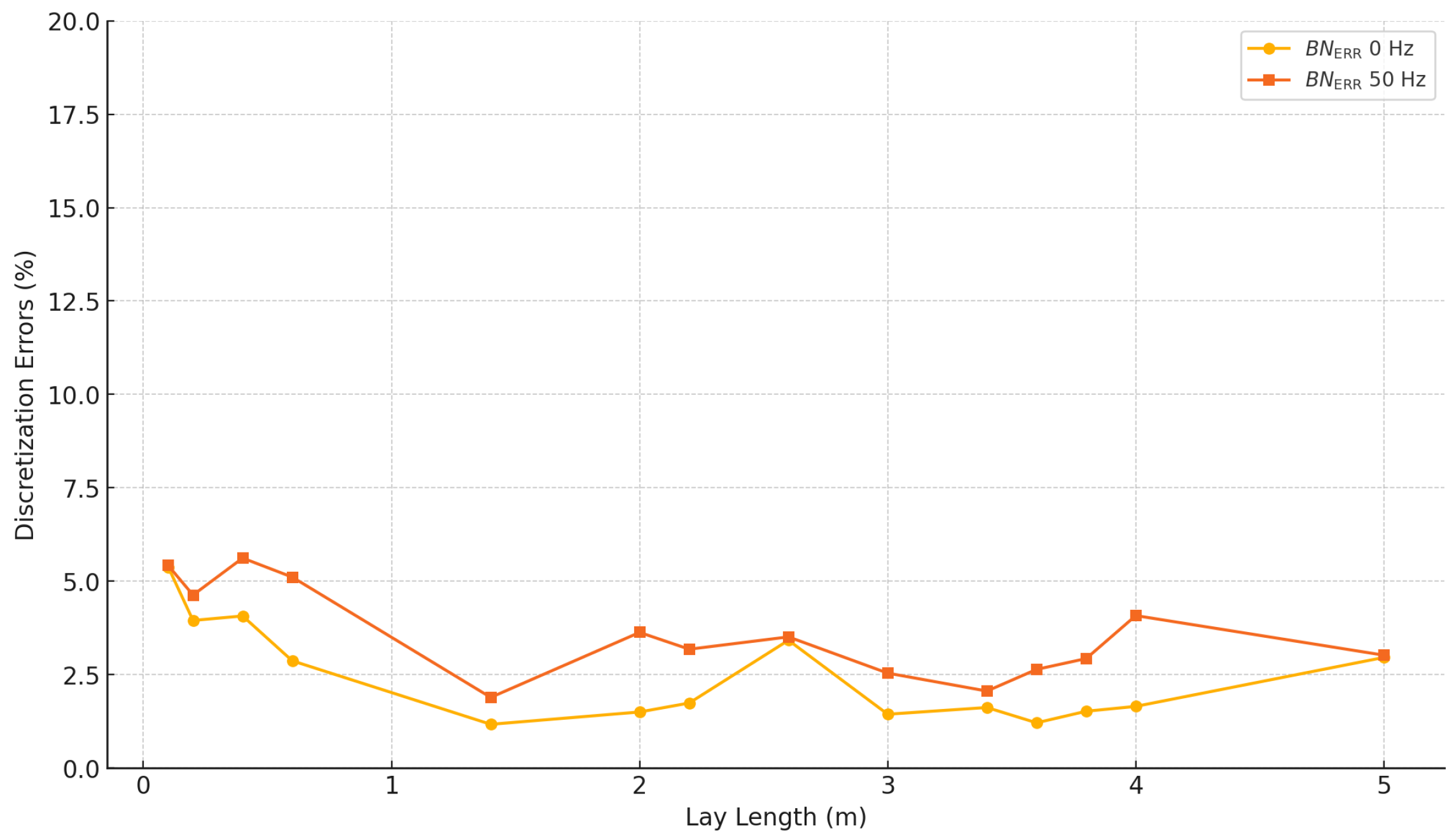
3.3. FE Error Estimates

Discretization errors occur when continuous electromagnetic fields are approximated using finite-element meshes. These errors are influenced by the mesh density and refinement, especially in regions with steep field gradients, such as near conductors and insulation layers. Adaptive meshing mitigates these errors by prioritizing critical regions, enhancing accuracy without significantly increasing computational demands. In ANSYS, the EMAGERR macro is commonly used to compute maximum discretization error norms, providing error estimates for electromagnetic field quantities like magnetic flux density (B). The $B{N}_{\mathrm{ERR}}$ represents a normalized metric indicating the discrepancy in flux density (B) values. Table 2 and Figure 6 shows error values for each of the 14 twisted models at 0 Hz and 50 Hz.

3.4. Boundary Conditions

Each twisted cable is excited at one end of the conductor segments with a total current of $I=10\mathrm{A}$, distributed equally among the five segments ($2\mathrm{A}$ per segment). The other end of each segment is set to ground (zero voltage). The external nodes of the surrounding air domain is enforced with a zero magnetic vector potential ($A_{\mathrm{Z}}=0$), approximating a sufficient far-field condition.

4. Two-Dimensional Benchmark Cases

In addition to the 3D twisted-cable models, two two-dimensional (2D) benchmarks are examined at 50 Hz:

• A solid circular conductor with the same cross-sectional area as the five-segment design;
• The five-segment model, corresponding to a 3D cable with an infinite lay length.

Both models are assumed to be infinitely long in the out-of-plane direction and consist of a copper region surrounded by 30 cm of air domain with material properties describe in Table 1. The following subsections briefly describe each benchmark’s geometry and the observed AC loss characteristics.

Table 3. Per-unit-length resistances for the two 2D benchmark cases at 50 Hz.

2D Model	${\mathit{R}}_{\mathbf{DC}-2\mathbf{D}}$ ($\mu \Omega /\mathbf{m}$)	${\mathit{R}}_{\mathbf{AC}-2\mathbf{D}}$ ($\mu \Omega /\mathbf{m}$)	$\frac{{\mathit{R}}_{\mathbf{AC}-2\mathbf{D}}}{{\mathit{R}}_{\mathbf{DC}-2\mathbf{D}}}$
Solid Round Conductor	6.36	11.72	1.843
Five-Segment	6.36	11.07	1.741

summarises the key parameters.

4.1. Solid Circular Conductor

The solid conductor has an identical section area to the 3D models which is $2711{\mathrm{mm}}^2$. When an AC current at 50 Hz is applied, the skin effect causes concentration of the current near the outer periphery, resulting in a non-uniform distribution. Figure 7a reveals the current density colour map, showing higher current density near the surface of the cable.

In Figure 7b, the light blue curve shows the current density in the solid round conductor under AC excitation at 50 Hz, plotted against the radial distance from the center. This profile highlights the skin effect, which forces the current toward the conductor’s outer periphery. By contrast, the purple horizontal line corresponds to the uniform current density that would be observed under DC conditions, where neither skin nor proximity effects distort the current distribution.

4.2. Five-Segment Conductor (Infinite Lay Length)

The second 2D model replicates the five-segment cross-sectional geometry used for the 3D simulations but with no helical twist, meaning that the sub-conductors remain perfectly parallel. This configuration represents the limiting case of a 3D cable with an infinite lay length. Under AC conditions at 50 Hz, both skin and proximity effects are present. The resulting current–density distribution shows enhanced non-uniformity near the outer layer of the cable as presented in Figure 8.

5. Results and Discussion

This section first analyzes the DC (0 Hz) results, confirming that $R_{\mathrm{DC}-2\mathrm{D}}/R_{\mathrm{DC}-2\mathrm{D}-\mathrm{cal}}=1.0$ irrespective of lay length. We then examine the 50 Hz outcomes, noting that $R_{\mathrm{AC}-2\mathrm{D}}/R_{\mathrm{DC}-2\mathrm{D}}>1$ and systematically increases with growing $\lambda$. Finally, an exponential-saturation curve is fitted to the 50 Hz results, and key physical interpretations are discussed.

5.1. DC Condition (0 Hz)

Under DC, the current distribution is uniform across each segment’s cross section, unaffected by skin or proximity effects [4].

Table 4. Power-loss calculations at 0 Hz (DC).

$\mathit{\lambda }$ (m)	${\mathit{P}}_{\mathbf{loss}}$ (mW)	${\mathit{R}}_{\mathbf{DC}}$ ($\mu \Omega$)	${\mathit{l}}_{\mathbf{twist}}$ (m)	${\mathit{R}}_{\mathbf{DC}}-2\mathbf{D}$ ($\frac{\mu \Omega }{\mathbf{m}}$)	${\mathit{R}}_{\mathbf{DC}}-2\mathbf{D}-\mathbf{cal}$ ($\frac{\mu \Omega }{\mathbf{m}}$)	$\frac{{\mathit{R}}_{\mathbf{DC}}-2\mathbf{D}}{{\mathit{R}}_{\mathbf{DC}}-2\mathbf{D}-\mathbf{cal}}$
0.1	0.1709	1.709	0.2688	6.36	6.36	1.00
0.2	0.1892	1.892	0.2975	6.36	6.36	1.00
0.4	0.2922	2.922	0.4594	6.36	6.36	1.00
0.6	0.4127	4.127	0.6490	6.36	6.36	1.00
1.4	0.9230	9.230	1.4513	6.36	6.36	1.00
2.0	1.3117	13.117	2.0625	6.36	6.36	1.00
2.2	1.4416	14.416	2.2668	6.36	6.36	1.00
2.6	1.7017	17.017	2.6758	6.36	6.36	1.00
3.0	1.9621	19.621	3.0852	6.36	6.36	1.00
3.4	2.2226	22.226	3.4948	6.36	6.36	1.00
3.6	2.3529	23.529	3.6997	6.36	6.36	1.00
3.8	2.4832	24.832	3.9046	6.36	6.36	1.00
4.0	2.6135	26.135	4.1096	6.36	6.36	1.00
5.0	3.2654	32.654	5.1346	6.36	6.36	1.00

shows the extracted total power loss at 0 Hz and total $R_{\mathrm{DC}}$ (in Ohms) for the 14 models. As each model has an effective length of $l_{\mathrm{twist}}$, the per-meter DC resistance $R_{\mathrm{DC}-2\mathrm{D}}$ is calculated by dividing the total $R_{\mathrm{DC}}$ by $l_{\mathrm{twist}}$. Naturally, the numerically calculated per-meter $R_{\mathrm{DC}-2\mathrm{D}-\mathrm{cal}}$ is constant at $6.36\mu \Omega /\mathrm{m}$. In all cases, $R_{\mathrm{DC}-2\mathrm{D}}/R_{\mathrm{DC}-2\mathrm{D}-\mathrm{cal}}=1.0$.

Physically, the difference in total power loss (in Watts) between small $\lambda$ and large $\lambda$ arises because the helix path is longer for larger $\lambda$ within each segment. However, when expressed as per-metre (i.e., normalising by $l_{\mathrm{twist}}$), the $R_{\mathrm{DC}-2\mathrm{D}}$ is the same for all models, confirming no difference in DC conduction (0 Hz) [1].

5.2. AC Condition (50 Hz)

At $50\mathrm{Hz}$, skin and proximity effects concentrate current near segment boundaries; moreover, the twisting modifies how segments interact over the cable length.

Table 5. Power-loss calculations at 50 Hz (AC).

$\mathit{\lambda }$ (m)	${\mathit{P}}_{\mathbf{loss}}$ (mW)	${\mathit{R}}_{\mathbf{AC}}$ ($\mu \Omega$)	${\mathit{l}}_{\mathbf{twist}}$ (m)	${\mathit{R}}_{\mathbf{AC}}-2\mathbf{D}$ ($\frac{\mu \Omega }{\mathbf{m}}$)	${\mathit{R}}_{\mathbf{DC}}-2\mathbf{D}$ ($\frac{\mu \Omega }{\mathbf{m}}$)	$\frac{{\mathit{R}}_{\mathbf{AC}}-2\mathbf{D}}{{\mathit{R}}_{\mathbf{DC}}-2\mathbf{D}}$
0.1	0.2263	2.263	0.2688	8.42	6.36	1.324
0.2	0.2898	2.898	0.2975	9.74	6.36	1.532
0.4	0.4846	4.846	0.4594	10.55	6.36	1.659
0.6	0.6974	6.974	0.6490	10.75	6.36	1.690
1.4	1.5798	15.798	1.4513	10.89	6.36	1.712
2.0	2.2495	22.495	2.0625	10.91	6.36	1.715
2.2	2.4732	24.732	2.2668	10.91	6.36	1.716
2.6	2.9206	29.206	2.6758	10.91	6.36	1.716
3.0	3.3685	33.685	3.0852	10.92	6.36	1.717
3.4	3.8165	38.165	3.4948	10.92	6.36	1.717
3.6	4.0405	40.405	3.6997	10.92	6.36	1.717
3.8	4.2646	42.646	3.9046	10.92	6.36	1.717
4.0	4.4887	44.887	4.1096	10.92	6.36	1.717
5.0	5.6095	56.095	5.1346	10.92	6.36	1.718

compiles the extracted total power loss in Watts, the total $R_{\mathrm{AC}}$ in Ohms, and the per-meter $R_{\mathrm{AC}-2\mathrm{D}}$ for each of the 14 models. The final column lists $R_{\mathrm{AC}-2\mathrm{D}}/R_{\mathrm{DC}-2\mathrm{D}}$.

A key observation is that all models have $R_{\mathrm{AC}-2\mathrm{D}}/R_{\mathrm{DC}-2\mathrm{D}}=R_{\mathrm{AC}}/R_{\mathrm{DC}}>1.0$, as theoretically expected ($R_{\mathrm{AC}}$ can never be below $R_{\mathrm{DC}}$). Notably, shorter lay lengths ($\lambda =0.1,0.2,0.4$ m) produce smaller $R_{\mathrm{AC}}/R_{\mathrm{DC}}$ (around 1.32–1.55), while longer lay lengths approach $\approx 1.70$–$1.72$.

These differences are attributed to how the magnetic fields from each segment interact along the twisted path. In the gently twisted scenario (large $\lambda$), each segment remains offset over a longer distance, enhancing local eddy currents near boundaries [11,12]; thus, $R_{\mathrm{AC}-2\mathrm{D}}$ is relatively higher. In a tightly twisted scenario, the segment alignment changes more rapidly, distributing the current distortion differently and leading to a somewhat lower $R_{\mathrm{AC}-2\mathrm{D}}$.

In the present model, each segment is considered a single solid region with no internal transposition as the individual conductor strings are not electrically insulated within segments, and it is only the five segments that are insulated by a relatively thin layer of air. The twisting primarily repositions entire segments around the z-axis passing through the cable’s center. In an individually insulated conductor scenario, the net effect can significantly alter electromagnetic coupling between conductors as well as segments, thereby impacting how current distributes at steady state.

5.3. Exponential-Saturation Model for $R_{\mathrm{AC}}/R_{\mathrm{DC}}$

To quantify how $R_{\mathrm{AC}}/R_{\mathrm{DC}}$ varies with lay length, we employ an exponential saturation model of the form:

$$y=c+a\left(1-e^{-bx}\right),$$

(5)

where y denotes $R_{\mathrm{AC}}/R_{\mathrm{DC}}$, x is the lay length $\lambda$, and c, a, and b are constants. Physically, we require $R_{\mathrm{AC}}/R_{\mathrm{DC}}\to 1$ as $\lambda \to 0$, so $c=1$. Fitting our simulation data yields (6).

$${\displaystyle \frac{R_{\mathrm{AC}}}{R_{\mathrm{DC}}}}=1+0.7157\left(1-e^{-6.3873\lambda }\right)$$

(6)

Equation (6) implies that as $\lambda$ becomes infinitely large, $R_{\mathrm{AC}}/R_{\mathrm{DC}}$ asymptotically approaches a value of $1.7157$.

Figure 9 illustrates this model fit. The green curve represents the exponential saturation relationship, while the markers show the finite-element simulation data. The near-complete overlap between the curve and the data points indicates a high coefficient of determination ($R^2\approx 0.9964$). A noteworthy verification step involved excluding the $\lambda =0.4\mathrm{m}$ data point during the curve-fitting process used to obtain the exponential-saturation relationship in (6). After determining the best-fit parameters without relying on that data point, we then evaluated how well the resulting model predicted the omitted $\lambda =0.4\mathrm{m}$ case. Specifically, the finite-element simulation yielded ${\mathrm{R}}_{\mathrm{AC}}/{\mathrm{R}}_{\mathrm{DC}}=1.659$, while the fitted equation gave a value of $1.6604$. The absolute difference is thus $0.0014$, which translates to a discrepancy of only $0.084\%$. Such a small error, even with the intentional exclusion of that point from the fitting procedure, illustrates the robustness and strong predictive capability of the model.

5.4. Total Cable Resistance vs. Per-Unit-Length Resistance

Before comparing the total AC resistance of different twisted configurations, we distinguish among three quantities: ${\mathrm{R}}_{\mathrm{AC}}$, which is the total AC resistance for a single twisted section of length $\lambda$; ${\mathrm{R}}_{\mathrm{AC}-2\mathrm{D}}$, the effective AC resistance per meter calculated by $R_{\mathrm{AC}-2\mathrm{D}}=R_{\mathrm{AC}}/l_{\mathrm{twist}}$; and ${\mathrm{R}}_{\mathrm{AC}-2\mathrm{D}-\mathrm{cable}}$, the per-meter resistance obtained by simply dividing ${\mathrm{R}}_{\mathrm{AC}}$ by $\lambda$.

Table 6. Presentation of resistance values for models with varying lay length $\lambda$ at 50 Hz.

$\mathit{\lambda }$ (m)	${\mathit{l}}_{\mathbf{twist}}$ (m)	${\mathit{R}}_{\mathbf{AC}}$ ($\mu \Omega$)	${\mathit{R}}_{\mathbf{AC}-2\mathbf{D}}$ ($\mu \Omega$/m)	${\mathit{R}}_{\mathbf{AC}-2\mathbf{D}-\mathbf{cable}}$ ($\mu \Omega$/m)
0.1	0.2688	2.263	8.42	22.63
0.2	0.2975	2.898	9.74	14.49
0.4	0.4594	4.846	10.55	12.12
0.6	0.6490	6.974	10.75	11.62
1.4	1.4513	15.798	10.89	11.28
2.0	2.0625	22.495	10.91	11.25
2.2	2.2668	24.732	10.91	11.24
2.6	2.6758	29.206	10.91	11.24
3.0	3.0852	33.685	10.92	11.23
3.4	3.4948	38.165	10.92	11.22
3.6	3.6997	40.405	10.92	11.22
3.8	3.9046	42.646	10.92	11.22
4.0	4.1096	44.887	10.92	11.22
5.0	5.1346	56.095	10.92	11.22

summarises these values for various lay lengths.

While the effective AC resistance per meter $R_{\mathrm{AC}-2\mathrm{D}}$ which is normalized by $l_{\mathrm{twist}}$, decreases for shorter lay lengths ($\lambda$), the actual AC resistance per meter of the cable, denoted $R_{\mathrm{AC}-2\mathrm{D}-\mathrm{cable}}$, can still be larger. The key distinction is that smaller $\lambda$ values create a more tightly wound helix, increasing the actual conductor path length within the same longitudinal distance. This tighter twist adds more conductor material to the total circuit, so charges must traverse a physically longer route—therefore incurring a higher total resistance. In other words, even if the per-unit-length resistance is reduced by improved current distribution (skin/proximity mitigation), the added conductor length can outweigh that benefit, leading to a greater overall ohmic loss for the entire longitudinal length of the cable. This relation is clearly visible in Figure 10.

6. Conclusions

In this work, a three-dimensional (3D) finite-element (FE) framework has been employed to accurately quantify how skin and proximity losses are influenced by varying lay lengths in multi-segment underground cables. Unlike simpler two-dimensional (2D) methods—which treat sub-conductors as though they are parallel—this 3D approach fully accounts for helical transposition. The key findings can be summarized as follows:

• Influence of Lay Length on AC Losses: Over the tested range of lay lengths (0.1 m–5.0 m at 50 Hz), the AC-to-DC resistance ratio ${\mathrm{R}}_{\mathrm{AC}}/{\mathrm{R}}_{\mathrm{DC}}$ varied from about 1.32 (for very tight twists) to nearly 1.72 (for gentle twists). This demonstrates that twisting can markedly change the current distribution and resultant AC losses;
• 3D FE Accuracy vs. 2D Simplifications: Two-dimensional models assume parallel sub-conductors and thus overestimate eddy-current losses, effectively treating lay length as infinite. By contrast, the proposed 3D model reveals how shorter lay lengths help redistribute current more uniformly;
• Exponential-Saturation Relationship: An exponential-saturation model was found to predict ${\mathrm{R}}_{\mathrm{AC}}/{\mathrm{R}}_{\mathrm{DC}}$ with high accuracy ($R^2\approx 0.996$) across all studied twists, offering a convenient analytical tool for cable designers;
• Total Cable Resistance vs. Per-Meter Perspective: Although the per-unit-length AC resistance is reduced at shorter lay lengths, the overall helical path is longer, which can increase the total cable resistance. Understanding both effects is key to balancing mechanical robustness with minimal AC losses.

Looking ahead, further studies may consider higher frequencies or transient phenomena, more complex conductor arrangements (e.g., partially insulated strands). Such advancements would continue to refine the design guidelines for high-voltage cables, helping manufacturers and regulators ensure that both mechanical and electromagnetic performance requirements are efficiently satisfied.

References

1. Okamura, S. Electrical Cables Handbook, 3rd ed.; Wiley: Hoboken, NJ, USA, 2017. [Google Scholar]
2. Lavers, J.L. Advanced Electromagnetic Analysis of Power Cables: Theory and Practice; IET Press: Stevenage, UK, 2020. [Google Scholar]
3. Paice, D.A. Skin effect in multi-layer conductors—The proximity effect. IEEE Trans. Power Appar. Syst. 1981, PAS-100, 1137–1145. [Google Scholar]
4. Gross, E.E. Proximity effect in systems of conductors. AIEE Trans. Power Appar. Syst. 1959, 78, 1352–1360. [Google Scholar]
5. Rosskopf, A.; Bär, E.; Joffe, C. Influence of Inner Skin- and Proximity Effects on Conduction in Litz Wires. IEEE Trans. Power Electron. 2014, 29, 5454–5461. [Google Scholar] [CrossRef]
6. Acero, J.; Lope, I.; Burdío, J.M.; Carretero, C. Loss Analysis of Multistranded Twisted Wires by Using 3D-FEA Simulation. In Proceedings of the Workshop on Control and Modeling for Power Electronics (COMPEL), Santander, Spain, 22–25 June 2014. [Google Scholar]
7. Reddy, P.B.; Jahns, T.M.; Bohn, T.P. Transposition Effects on Bundle Proximity Losses in High-Speed PM Machines. In Proceedings of the 2009 IEEE Energy Conversion Congress and Exposition, San Jose, CA, USA, 20–24 September 2009; pp. 1919–1926. [Google Scholar]
8. Sullivan, C.R.; Zhang, R.Y. Analytical Model for Effects of Twisting on Litz-Wire Losses. In Proceedings of the 2014 Conference on Magnetics and Power Electronics, Santander, Spain, 22–25 June 2014. [Google Scholar]
9. Plumed, E.; Acero, J.; Lope, I.; Carretero, C. 3D Finite Element Simulation of Litz Wires with Multilevel Bundle Structure. In Proceedings of the IECON 2018—44th Annual Conference of the IEEE Industrial Electronics Society, Washington, DC, USA, 21–23 October 2018. [Google Scholar]
10. Piwonski, A.; Dular, J.; Rezende, R.S.; Schuhmann, R. 2-D Eddy Current Boundary Value Problems for Power Cables with Helicoidal Symmetry. IEEE Trans. Magn. 2023, 59, 6300204. [Google Scholar] [CrossRef]
11. Morgan, R.B.; Fink, D.G. Method for computing skin and proximity effects in cable conductors. IEEE Trans. Power Appar. Syst. 1975, 94, 344–354. [Google Scholar]
12. International Electrotechnical Commission. IEC 60287: Electric Cables—Calculation of the Current Rating; International Electrotechnical Commission: Geneva, Switzerland, 2020. [Google Scholar]
13. Brauer, J.R. Magnetic Actuators and Sensors; IEEE Press: New York, NY, USA, 2006. [Google Scholar]
14. Saldanha, N. High-frequency modeling of power cables. IEEE Trans. Power Deliv. 2013, 28, 247–256. [Google Scholar]
15. Khan, S.; Grattan, K.T.V.; Attwood, J.R. Finite Element Modelling of Skin and Proximity Effects in High Voltage Power Cables. In Proceedings of the COMPUMAG, Evian, France, 2–5 July 2001; pp. 2–5. [Google Scholar]
16. Silva, F.J. Power Cables and Their Applications; Springer: Berlin/Heidelberg, Germany, 2013. [Google Scholar]
17. McAllister, R. Handbook of Electrical Engineering Calculations; McGraw-Hill: New York, NY, USA, 1982. [Google Scholar]
18. ANSYS Inc. ANSYS Electromagnetics Documentation; ANSYS Inc.: Canonsburg, PA, USA, 2022. [Google Scholar]
Figure 1. Five-segment cable cross-section (2D view) used for extruding 3D cables. Each segment is treated as a solid bundle of hexagonally packed strands. All dimensions are in meters.
Applsci 15 02814 g001
Figure 2. Three-dimensional extruded model of the five-segment cable with parallel (no twisting) sub-conductors.
Applsci 15 02814 g002
Figure 3. A schematic representation of the five-segment cable twisted around the z-axis.
Applsci 15 02814 g003
Figure 4. Developing the 3D twisted geometry process staring from the 2D 1 / 5 slice model (a), 3D 1 / 5 slice conductor (b), 3D 1 / 5 slice conductor with air (c) and the full model volume (d).
Applsci 15 02814 g004
Figure 5. Helical path of length l twist for one 360 revolution, with lay length λ along the z-axis and distance r normal to the z-axis.
Applsci 15 02814 g005
Figure 6. BNERR error across different models at 0 Hz (DC) and 50 Hz.
Applsci 15 02814 g006
Figure 7. Two-dimensional results for the solid-round-cable current density J ( A / m 2 ) at 50 Hz, presented as a colour map (a) and plotted along the path shown in the colour map (b).
Applsci 15 02814 g007
Figure 8. Colour map of the current density J ( A / m 2 ) at 50 Hz for the 5-segment model in 2D.
Applsci 15 02814 g008
Figure 9. Ratio R AC / R DC vs. lay length ( λ ) with exponential-saturation fit (green curve). The data points are extracted from the 3D FE simulations.
Applsci 15 02814 g009
Figure 10. Visualising the change in R AC - 2 D and R AC - 2 D - cable as ley length varies.
Applsci 15 02814 g010