Abstract
The attenuation of resonant frequencies across the entire spectrum of an audio signal is important because it helps to eliminate the harshness, sibilance, clear muddiness, boominess, and proximity effect of any sound source. This paper presents a method for the attenuation of resonant frequencies across the entire spectrum of an audio signal. A spectrum obtained by the Fast Fourier Transform is segmented into bands—one-third octave bands and Equivalent Rectangular Bandwidth-scale bands—in order to obtain the maximum value per band. Additionally, a curve representing the general shape of the spectrum is generated using the standard deviation to create a threshold curve for detecting resonant frequencies. The array with maximum values per bands and the array with the threshold curve are used to detect the resonant frequencies and calculate the attenuation for each filter. Subsequently, the coefficients of a second-order section of IIR-Peak filters are calculated for processing the input signal. Twenty audio files from different sources are utilized to test the algorithm. The output produced is then compared to that produced by the commercially available Soothe2 and RESO plug-ins. The Root Mean Square Level and the Loudness Units Full Scale integrated metrics are reported. The proposed plug-in output is more attenuated than the output from commercial plug-ins under factory conditions. The average RMS attenuation is −2.32 dBFS, while Soothe2 and RESO exhibit −1.27 dBFS and −1.10 dBFS, respectively. The attenuation per octave band over time is calculated using the Wavelet Transform. Finally, an annotator agreement used as a subjective result is made with 40 people related to audio and music in order to verify if the attenuation generated by the present work at resonant frequencies agrees with subjective opinion. The octave band analysis and annotator agreement show that the proposed plug-in performs better on audio from vocal, percussion, and guitar ensembles.
1. Introduction
An equalizer is a tool utilized for manipulating the spectral characteristics of an audio signal, including the amplitude and phase of the signal. In contrast, a dynamic process modifies the amplitude and envelope of a signal. Equalization changes amplitude in the frequency domain, whereas dynamic processors alter amplitude in the time domain [1]. Consequently, a dynamic equalizer modifies the frequency response curve of an audio signal in accordance with the input signal only under certain conditions. A condition is when the input signal exceeds or falls below a predefined threshold. The dynamic equalizer may find specific use in the protection/enhancement of professional audio equipment [2].
The discipline of digital signal processing enables the design and development of automated tools to address complex problems. Digital signal processing technology makes it possible to design effects with greater complexity and precision. For instance, effects based on analysis/synthesis techniques can be applied in real time [3]. Before automated tools, only professionals in the field were able to provide partial solutions to these problems with simple tools. One example of manual processing is the attenuation of resonant frequencies in audio files. In Bitzer et al. [4], twenty-two mixing engineers with different levels of experience were asked to identify and reduce the amplitude of frequencies they deemed resonant with a parametric equalizer in 16 audio files exhibiting frequency defects. The results demonstrated that the overall agreement in the narrowband analysis was less than 50%. This indicates that manually detecting and attenuating frequency resonances represents a significant challenge for audio engineers. In addition, a static equalizer is unable to attenuate resonant frequencies in an audio file, given that the harmonic components of sound change over time. There are two types of static equalizers: parametric and graphic. The parametric equalizer allows the operator to add a peak or a notch at an arbitrary location in the audio spectrum, making it the most flexible of the different types of equalizers. In parametric equalizers, multiple sections are typically connected in cascade [5]. Midrange bands in a parametric equalizer have three parameters: gain, center frequency, and bandwidth. Graphic equalizers are a fixed set of equalizers, where the center frequencies and bandwidths are preset and only gain is adjustable [5]. Common graphic equalizer designs have approximately 30 filters, which can be used to manipulate the frequency response of each audio [1]. In contrast, dynamic equalizers apply frequency amplitude processing with static thresholds. Dynamic equalizers enable conventional equalizers to modify the equalization curve in a manner that is responsive to time. This is made possible by their incorporation of dynamic range compressor parameters, including threshold, ratio, and, in certain instances, attack and release. The equalization stage is able to respond dynamically to the input signal level [1].
A limited number of plug-in equalizers function as resonance suppressors in audio files. An audio plug-in is a collection of software programs that process an audio signal [6]. These programs have their own graphics module for on-screen display. Some commercial plug-ins that have the function of attenuating resonant frequencies are Soothe2 [7] developed by oeksound and RESO [8] developed by Mastering the Mix.
Soothe2 is a dynamic resonance suppressor that is capable of automatically detecting resonances over the entire frequency range. The software is capable of identifying problematic resonances in real time and applying corresponding reductions automatically.
RESO is a dynamic resonance suppressor that is designed to analyze and identify specific frequencies that exhibit energy buildup. It then proposes nodes in the spectrum that work as static equalizers, which reduce the amplitude at certain frequencies. The algorithms and code behind the these commercial resonance suppressor plug-ins are not available to the general public.
To the best of our knowledge, academic results on detecting and attenuating resonant frequencies for audio files across the spectrum are scarce. In Corbach et al. [9], a system for detecting resonances in a room using the Fast Fourier Transform (FFT) and Peak filters is presented. The system plays a signal through loudspeakers, captures it with a microphone, and digitizes it. In the case of digital audio, the signal is analyzed with respect to the generated signal and the coefficients of the filters are calculated in order to attenuate the resonances. This system works at frequencies below 200 Hz and proposes the use of static filters.
Some algorithms for resonant frequency detection employ the FFT to perform a frequency domain analysis. In Wakefield, J. [10], an algorithm is developed that uses the magnitude spectrum, whereby the highest values from each sample section are identified and the five highest peaks from the entire audio file are selected. These peaks are considered the resonances of the audio signal if the value is higher than the FFT bin for either side of it for the audio region. A more complex algorithm was proposed by Bitzer et al. [11] where spectrum normalization is performed and two spectrum curves are created: a fine structure curve and a general shape curve of the signal. By splitting the spectrum, the amplitude of all frequencies is matched with the smoothed spectrum, and the maximum peaks in the fine structure can be obtained. Finally, the highest peaks of the signal are identified as resonant frequencies.
A comparable study is presented by Presti [12], in which a prototype for automatic and real-time compensation of the psychoacoustic frequency masking effect is developed. In the study, a 32-band dynamic equalizer based on the Bark psychoacoustic scale is employed. The prototype analyzes a control signal and generates a masking threshold curve, which is then used to adjust the equalizer so that the spectrum curve of the input signal aligns with the designed control signal. It is noteworthy that the program is designed as an audio plug-in with a specific buffer size of 1024 samples, ensuring real-time functionality.
This paper proposes a method to detect and attenuate resonant frequencies in an audio signal. An amplitude dynamic equalizer with thirty bands and dynamic thresholds is designed. In order to identify the resonant frequencies of the input signal, a frequency domain analysis is conducted, using the magnitude spectrum obtained by the FFT. With the magnitude spectrum of the signal, representative values for each of the thirty bands are obtained. Two frequency band distributions are proposed: one by one-third octave bands and the other by the psychoacoustic scale according to Equivalent Rectangular Bandwidths (ERBs). The scale is selected based on the Spectral Flatness coefficient. The maximum value for each of the thirty bands is then obtained using the amplitude spectrum with the band distribution.
The empirical rule of the standard deviation is proposed for the analysis of spectral data. This rule states that 95% of all values in a dataset lie within two standard deviations from the mean [13]. The value of four standard deviations for each octave band is then calculated and linearly interpolated across the center frequencies of the band distribution. The resulting algorithm then generates a curve that approximates the general shape of the spectrum, disregarding the peaks of the signal.
The difference between the array of maximum values and the array with the threshold curve is obtained for each of the thirty bands. The attenuation per band is calculated by taking the average of the difference between each matrix and the previously calculated difference. If this is the first iteration, the same value is retained. The attenuation calculated between the average of the difference of the two arrays is used to calculate the coefficients of the filter bank with thirty second-order Peak IIR filters to process the input signal. These kinds of filters are used to control a narrower frequency band: they produce a bell-shaped curve affecting only the frequencies in a specific range [5]. According to Välimäki and Reiss [1], in a typical equalizer, all sections are composed of second-order Peak filters because these filters produce smooth transitions that are advantageous in that the effect of equalization is subtle and not perceived as an artifact. The input signal is processed through a second-order filter section with the objective of attenuating resonant frequencies that fall outside the threshold curve (which has the general shape of the spectrum) of the input signal. This is achieved in order to smooth out artifacts in the input signal.
Twenty audio files from different sources obtained from various multitracks from the Mixing Secrets For The Small Studio - Additional Resources library by Cambridge Music Technology are analyzed to compare the response of our work with the response of commercial plug-ins. The amount of attenuation obtained according to the Root Mean Square (RMS) level and Loudness Units Full Scale (LUFS) metric is analyzed. An octave band analysis is also conducted using the Wavelet transform to obtain a logarithmic spectrogram of the frequencies over time of each signal. This analysis allows for the attenuation produced by each plug-in to be quantified. The attenuation is expected to be in the range of −10 dB to −0.25 dB, since the human ear can detect minimal changes of 0.25 dB at high levels [14]. If a sound is reduced from 6 dB to 10 dB, the human ear will perceive this reduction as half the loudness of the original sound and this will affect the harmonic content of the audio signal [15]. It is important to analyze the most sensitive frequencies of the human ear, between 1 kHz and 4 kHz, based on the equal loudness curves [6].
To confirm that the attenuation was indeed at resonant frequencies, a scorer’s agreement was made. In this agreement, 40 people involved in audio and music were asked if the perceived attenuation was at resonant frequencies in different frequency ranges. Seventy-four percent of respondents confirmed that such attenuation occurs at resonant frequencies.
The method’s contribution lies in its capacity to adapt to any type of audio input. It is developed as an audio plug-in in Virtual Studio Technology (VST) format. The VST format was developed by Steinberg in 1996 and is currently the most widely supported format within the majority of Digital Audio Workstations (DAWs) currently available on the market. As mentioned by Martignon [2], in order to go beyond some limitations imposed by the use of commercial tools, the use of audio plug-ins allows direct comparison with these commercial tools due to the VST standard. Finally, it offers a higher attenuation than other plug-ins in factory conditions, with a resonant frequency detection response similar to Soothe2 because they both analyze the input signals over time and apply attenuation automatically.
The rest of this paper is organized as follows. Section 2 provides a detailed description of the proposed method. Section 3 outlines the experimental procedures and presents a comparative analysis between the proposed method and other commercial tools. Finally, Section 4 presents a discussion of the results and conclusions.
2. Materials and Methods
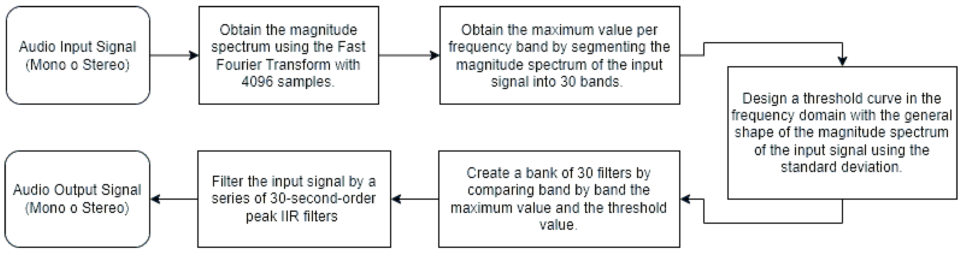
Figure 1 illustrates the proposed method, which comprises four main steps: determine a representative value for each frequency band, design a threshold curve, create a filter bank, and filter the input signal. A frequency domain analysis of the input signal is carried out via the Fast Fourier Transform (FFT). The input signal is analyzed in the frequency domain using the FFT algorithm, which allows the spectral behavior of the signal to be determined and the attenuation required for each band to be calculated. This information is then used to design an audio filter bank for each frequency band. Finally, filters are applied to the input signal to attenuate the resonant frequencies.
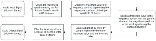
Figure 1.
A general block diagram of the system.
2.1. Input Signal Preprocessing
Within the context of an audio plug-in, the input signal is expressed as a finite digital signal. This signal is represented in floating point format, with values between −1 and 1 with levels depending on the bit depth. The signal is represented as a matrix of N samples for each of the audio channels. For monophonic signals, this is one channel; for stereophonic signals, this is two channels. This matrix is known as the input buffer. The number of samples depends on the buffer size (N) determined by the user in the audio interface and in the digital audio workstation (DAW) where the plug-in is hosted. The size of the input buffer is typically one of the following values: 128, 256, 512, or 1024 samples. Buffer size is defined based on computing power and latency. Low buffer sizes result in lower latency but more processing power, while high buffer sizes result in higher latency but less processing power.
Once the signal has been stored in the input buffer, the data are transferred to a vector (referred to as the analysis buffer) with a greater number of samples than the input buffer. This vector is utilized for further processing. The analysis buffer was designed to contain a greater number of samples than the input buffer in order to have more information from the input signal for analysis. The size of the analysis buffer was set to 4096 samples, which is a multiple of the common input buffer sizes. The greater the number of samples analyzed, the greater the resolution between frequencies.
The analysis buffer stores the input signal in a manner that considers only one channel. When the signal is monophonic, the stored values are identical to those of the input signal. Conversely, in the event that the signal is stereophonic, the buffer stores only the central portion of the signal, which is obtained by averaging the values present in the left and right channels. The analysis buffer still contains values between −1 and 1 in floating point as it is a representation of the input signal.
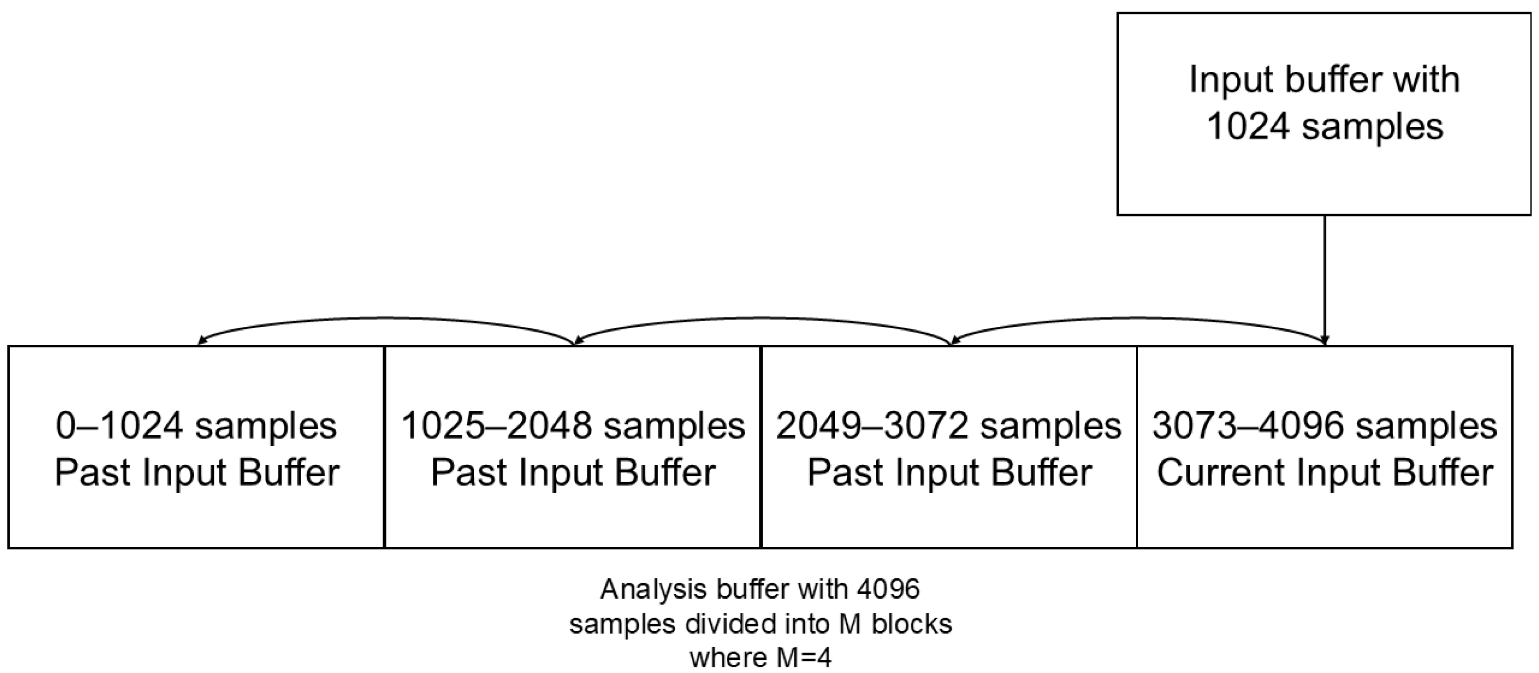
The initialization of the analysis buffer is set to zero. The analysis buffer is segmented into blocks of dimensions identical to those of the user-defined input buffer. The data are transferred by shifting the analysis buffer through a cycle with M steps, where M corresponds to the number of blocks in the analysis buffer. In cases where the input buffer contains 128 samples, M will be 32, while in instances where the input buffer comprises 1024 samples, M will be 4, as shown in Figure 2. This process results in the second block being stored in the first, the third in the second, and so on, until the last block is stored in the penultimate one. In the final block, the input buffer is stored, containing the current signal and the past samples.
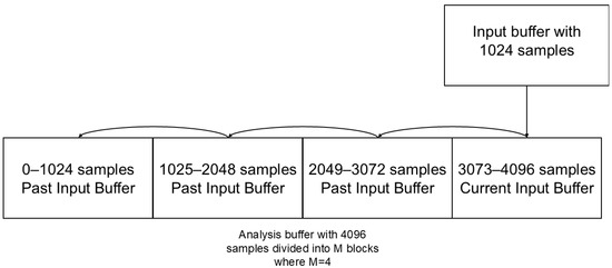
Figure 2.
Representation of the analysis buffer with respect to the input buffer with a sample size of 1024 samples.
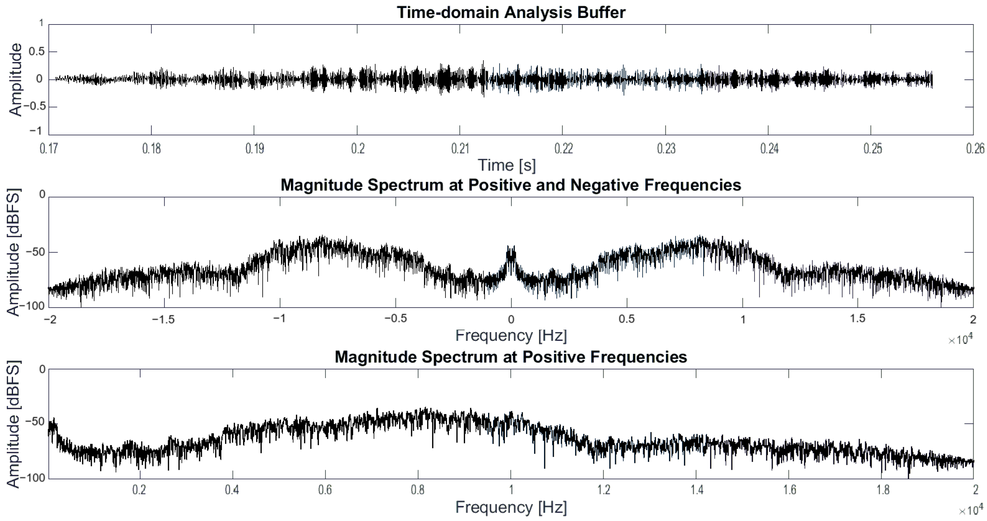
The Discrete Fourier Transform (DFT) of the signal stored in the analysis buffer is obtained using the FFT algorithm. The Fast Fourier Transform (FFT) was computed using MATLAB R2022a FFT function. The function accepts an input array x with double, single, or int format values and delivers the frequency domain representation returned as a vector. In this case, the function returns an array of complex numbers, representing each complex exponential by discrete frequencies. Subsequently, the magnitude spectrum of the signal is obtained by calculating the magnitude of each complex exponential. Furthermore, the non-reflected spectrum is obtained in order to have a representation of the signal from the origin to the Nyquist frequency. The magnitudes of the complex exponentials obtained in the FFT are subsequently normalized by dividing each amplitude by the total sample value, thereby ensuring that the magnitude spectrum is within the range of zero to one. Figure 3 shows in the first section the analysis buffer of a part of some audio corresponding to a voice; in the second section, the spectrum of the signal is shown. Finally, the third section shows only the magnitude spectrum from the origin at 22 kHz.
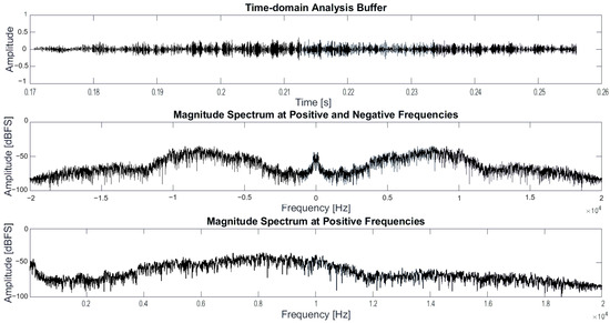
Figure 3.
Time-domain analysis buffer, magnitude spectrum at positive and negative frequencies, and magnitude spectrum at positive frequencies.
2.2. Representative Values
The determination of the bands is based upon a frequency scale selected according to a criterion defined by the Spectral Flatness measure as shown in Equation (1). The Spectral Flatness coefficient is a metric employed to characterise an audio spectrum. It provides a quantitative means to ascertain the extent to which a sound resembles a pure tone, as opposed to being noise-like. In order to obtain a representative value per band, it is necessary to define the frequency band distribution. These parameters determine the center frequency and the bandwidth for signal analysis and filtering. Thirty frequency bands are considered and two types of frequency band distributions are proposed.
The discrete function is the amplitude in frequency band number n and N is the total number of spectrum samples.
The first distribution is in one-third octave bands, using 100 Hz as the reference. From there, the frequencies from 25 Hz to 20,000 Hz are calculated using Equation (2), where is the reference frequency and is the next frequency on the scale. Bandwidths are defined by the standard in [16], which defines the distribution of the auditory spectrum by fractions of an octave using a reference center frequency.
The second proposed distribution is the Equivalent Rectangular Bandwidth (ERB) psychoacoustic scale. Each band of such a scale is based on auditory critical bands [17]. For the distribution, it is necessary to calculate the band spacing overlap factor v, which is defined by the extreme frequencies and the number of bands given by Equation (3) [17]; is the lowest frequency of the auditory spectrum corresponding to 20 Hz, is the highest frequency of the auditory spectrum corresponding to 20,000 Hz, and N is the number of bands corresponding to 30.
The superposition factor v is used to calculate the center frequencies for each band using Equation (4), where is the center frequency and n = 1, …, 30 to obtain the center frequencies.
Finally, Equation (5) is used to calculate the bandwidths for each center frequency.
It is known that the bandwidth is given by the difference between the upper frequency and the lower frequency of the band as and the center frequency is given by the geometric mean between the two extremes of the band—. With these equations, the expressions for each frequency are given by Equations (6) and (7).
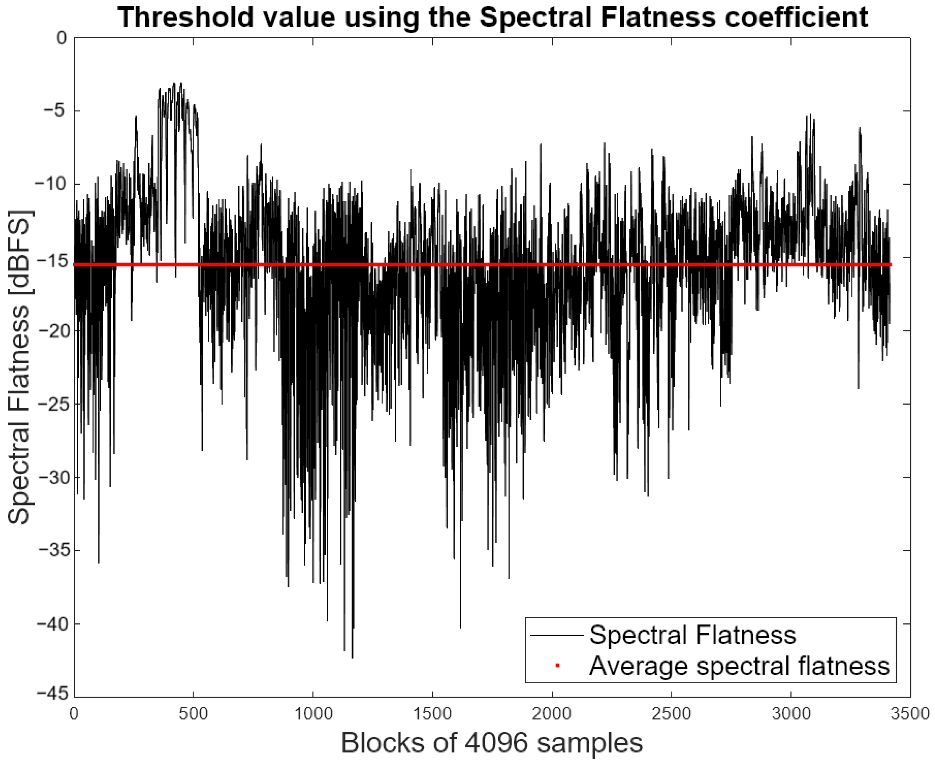
The Spectral Flatness measure in decibels as shown in Equation (1) is employed to select a scale. The coefficient serves to quantify the degree of resonance exhibited by the signal spectrum. A high coefficient (approaching 0 dB) indicates that the spectrum exhibits a similar power distribution to white noise. In the opposite case, the power is concentrated in certain bands, similar in characteristics to a pure tone [18]. A threshold was determined for the choice between the third octave distribution and the ERB scale. The threshold was calculated by dividing all the audio files in the dataset into blocks of 4096 samples and obtaining the spectral flatness coefficient for each block. Finally, the average of all blocks was calculated, and the threshold was determined. The coefficient value for each block and the average value, which is considered the threshold, are shown in Figure 4. The resultant threshold was −15 dB.
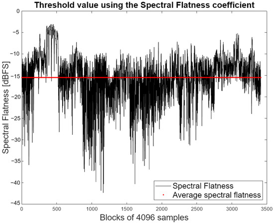
Figure 4.
Spectral Flatness coefficient values for the audio files used to obtain the threshold value between frequency distributions.
In scenarios where the input signal exhibits an equivalent power concentration across the spectrum, i.e., where the Spectral Flatness coefficient exceeds the threshold, the distribution by thirds of an octave is employed, as it exhibits a coherent bandwidth throughout the spectrum. In contrast, when the coefficient falls below the threshold, the ERB distribution is used, as it allows the bandwidth to vary throughout the spectrum.
Figure 5 illustrates that for center frequencies below 500 Hz, the behavior is linear, while for higher frequencies, it resembles a logarithmic behavior by sixths of an octave (i.e., with a smaller bandwidth).
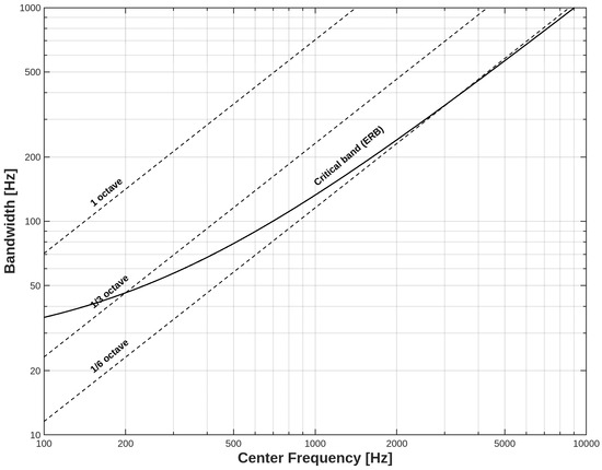
Figure 5.
Bandwidth distribution of octave, octave thirds, octave sixths, and ERB scales [6].
A buffer of 4096 samples is used to analyze the input signal in the frequency domain. The FFT is applied to the analysis buffer to obtain the normalized magnitude spectrum, which is then divided by bands according to a previously chosen distribution. Finally, the representative value per band is the maximum value of the group.
2.3. Threshold Curve with Standard Deviation
The magnitude spectrum is used to generate a curve that approximates the shape of the audio spectrum, while disregarding the peaks of the signal. This is achieved by applying the standard deviation rule of thumb, which states that 95% of a group of data is between two times the standard deviation above the mean and two times the standard deviation below the mean [13]. The standard deviation is calculated by octave bands, and each value is multiplied by four because the spectrum is normalized. The calculated value is then taken as a threshold. The threshold values per octave band are converted to decibels as shown in Equation (8).
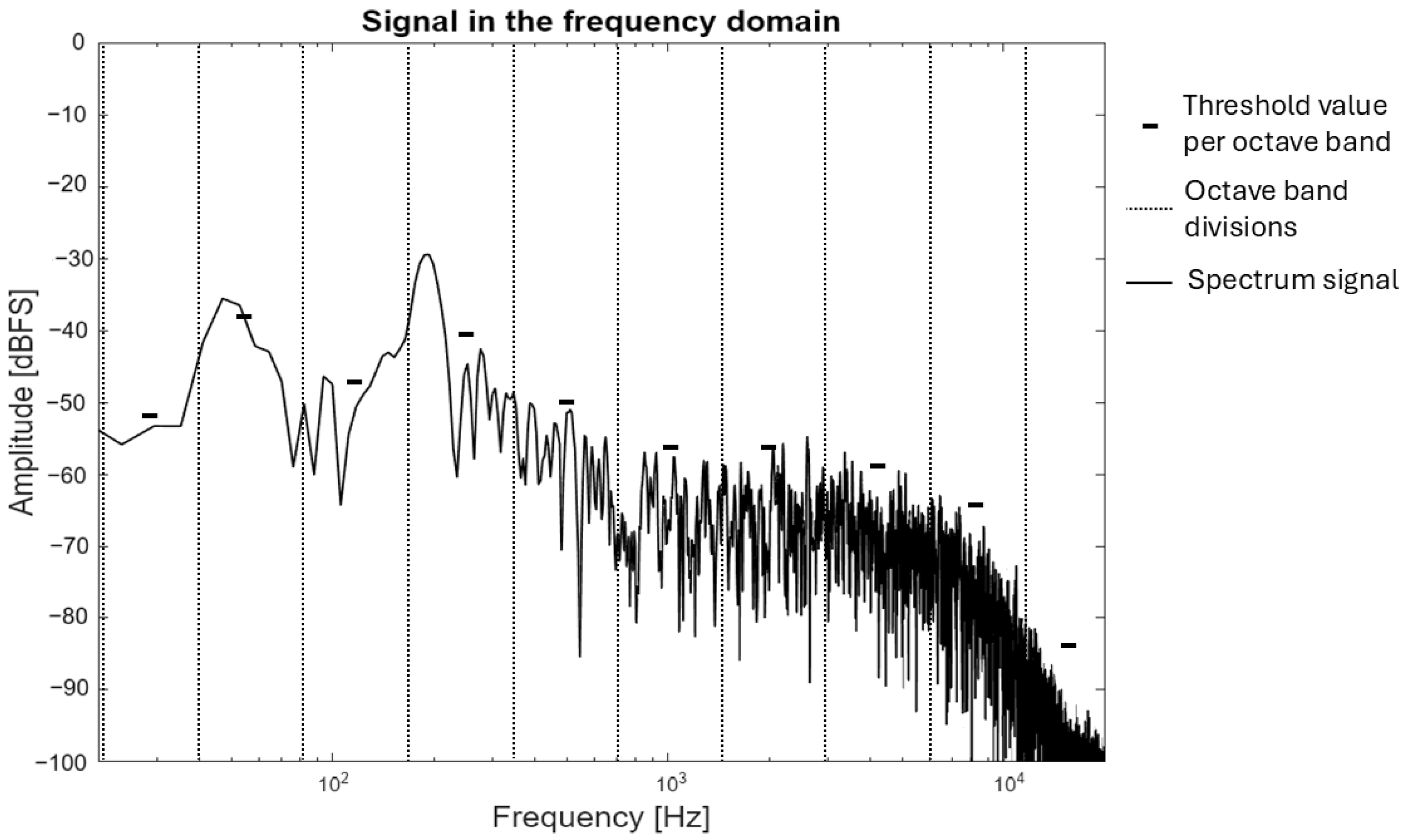
The function is the amplitude for a frequency band number, N is the number of frequencies in an octave band, and is the mean amplitude corresponding to the frequencies within an octave. As demonstrated in Figure 6, the spectrum is divided into octave bands, and the threshold values obtained with Equation (8) are presented. This equation facilitates the calculation of a threshold value that considers the amplitudes of the corresponding band, while disregarding the prominent peaks.

Figure 6.
Magnitude spectrum divided by octave bands to obtain threshold per octave.
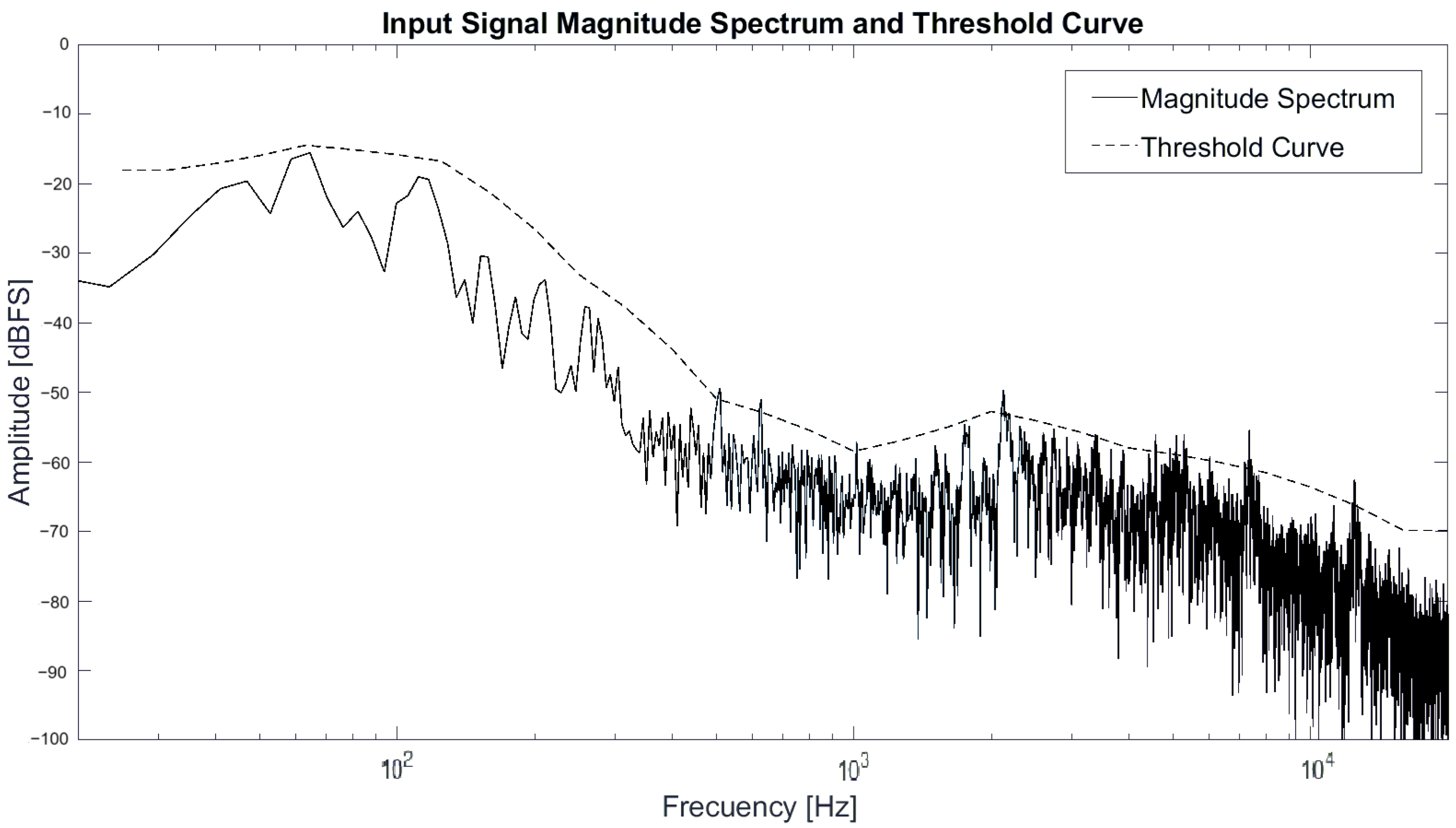
With each representative value per octave, a linear interpolation is performed along all center frequencies of the distribution calculated in Section 2.2 within the range of 31.5 Hz to 16,000 Hz. Values that fall outside the specified range are maintained at the same value at both ends; for example, the octave value of 31.5 Hz is identical for lower frequencies, and likewise, values for frequencies above 16 kHz will have the same value as that frequency, as shown in Equation (9). Figure 7 shows the threshold curve generated by interpolating the 30 points of the center frequency of the selected distribution.
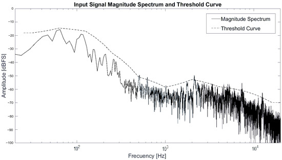
Figure 7.
Magnitude spectrum of drum audio input signal and threshold curve generated from spectrum using standard deviation.
The function is the amplitude corresponding to a frequency f, is the center frequency corresponding to each band where n = 1, …, 30, and and are the lower and upper frequencies per octave band, respectively, whose value depends on the value of .
Thus, an arrangement with a threshold curve that only considers the general shape of the spectrum is obtained. Figure 7 illustrates the spectrum of a drum signal at a specific instant, at which point the magnitude spectrum and the threshold curve are calculated.
2.4. Filter Bank and Signal Filtering
The arrays obtained in the sections of the maximum representative value per band (see Section 2.2) and the smoothed threshold curve of the input signal spectrum (see Section 2.3) are employed to ascertain the resonant frequencies by calculating the attenuation per band required to smooth the spectrum.
Consequently, a cycle is made to go through the arrays in order to perform a node by node comparison. In the event that the value of the maximum amplitude exceeds the threshold curve, the subtraction between the threshold and the maximum is obtained; otherwise, a value of zero is assigned. The two arrays are vectors of dimension 30, corresponding to one value for each band. Each vector contains the relevant spectrum information. The first vector has the maximum value per band in decibels, with negative float values. The second vector is the threshold curve vector, which has 30 floating point values in decibels less than 0. The difference array is employed to determine the attenuation that each filter will process. This calculation is conducted by averaging the preceding values and the current values. The averaging process serves to mitigate abrupt changes between each sample buffer. The final attenuation vector is converted from decibels to linear scale, resulting in a vector of dimension 30 with values between 0 and 1 in floating point, thereby representing the attenuation for each frequency band.
The implemented filter is a second-order IIR-Peak-type filter proposed in Välimäki et al. [1], which is described as follows: for gain G greater than one, it increases the gain in the operating band; for G between zero and one, it attenuates the signal. The bandwidth is specified by the quality factor and has a center frequency . It is satisfied that outside the operating range, it has a unity gain. Furthermore, the filter exhibits unity gain in the limit where the frequency is zero and in the Nyquist limit (at half the sampling frequency, ). This type of equalizer is employed due to its minimal computational expense and latency. Equalizers exhibiting these attributes are referenced as parametric EQs, graphic EQs (IIR), analog-matched EQs, and dynamic EQs [1] and most of these equalizers use this type of filter. The Z-domain transfer function of the filter is described by Equation (10).
In accordance with the provided Equations (11)–(13), the coefficients , , and correspond, respectively, to the first, second, and third coefficients of the numerator of the filter transfer function in the Z-domain. Similarly, in Equations (14)–(16), the coefficients , , and correspond, respectively, to the first, second, and third coefficients of the denominator of the filter transfer function in the Z-domain; see Equation (10).
In the following equation, Equation (17), is the digital angular frequency that depends on the center frequency and the sampling frequency .
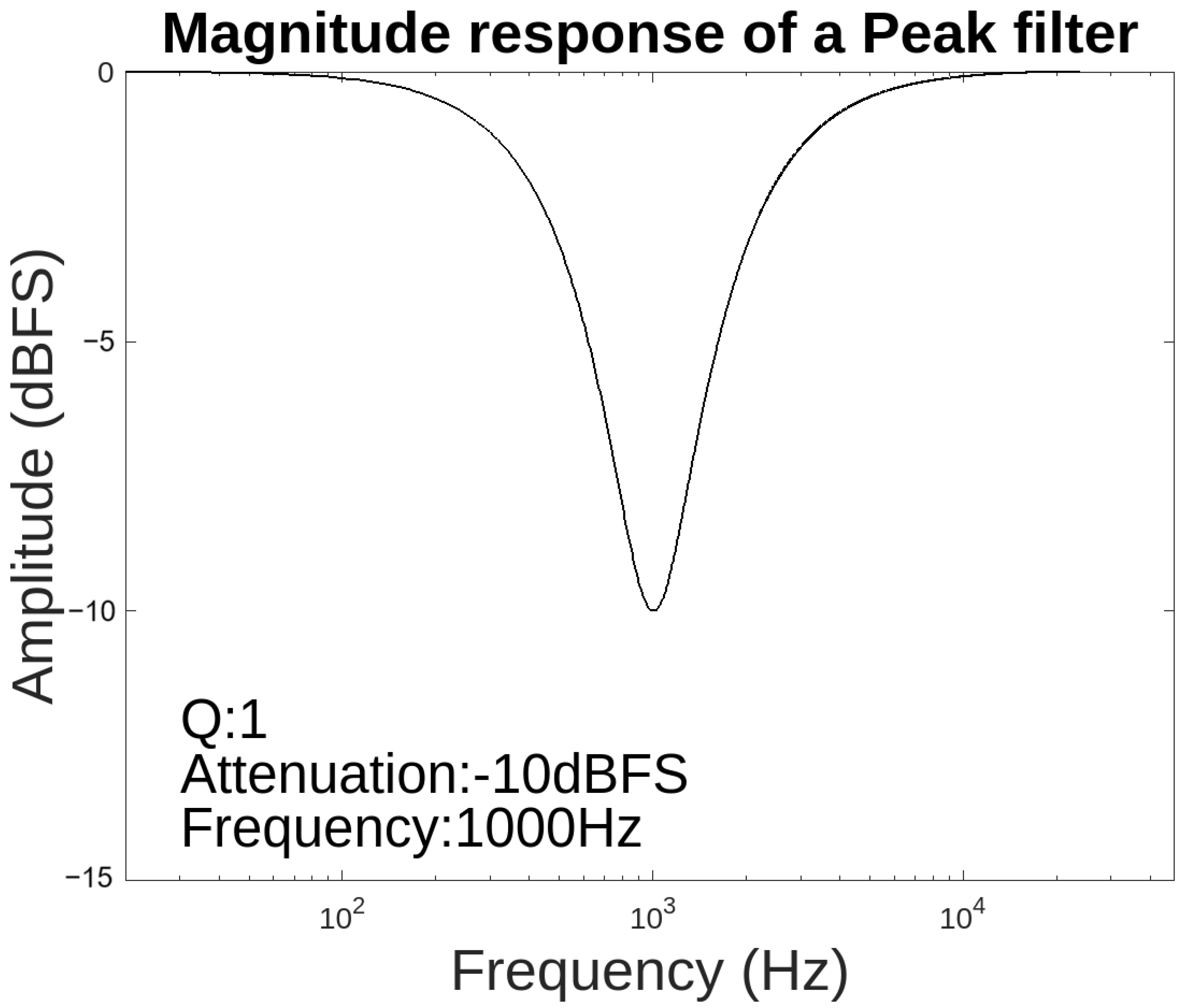
The magnitude response of a Peak filter is illustrated in Figure 8 when the Q (Bandwidth) factor is 1, the G value corresponding to the attenuation is −10 dBFS, and the centre frequency is 1000 Hz.

Figure 8.
Magnitude response of Peak filter.
In order to calculate the coefficients of each filter, it is necessary to have the center frequency , the bandwidth , and the attenuation G. The center frequency and bandwidth are defined by the band distribution chosen in Section 2.2, while the attenuation is that calculated by the average between the current and past difference of the arrays with the maximum values per band and the threshold curve.
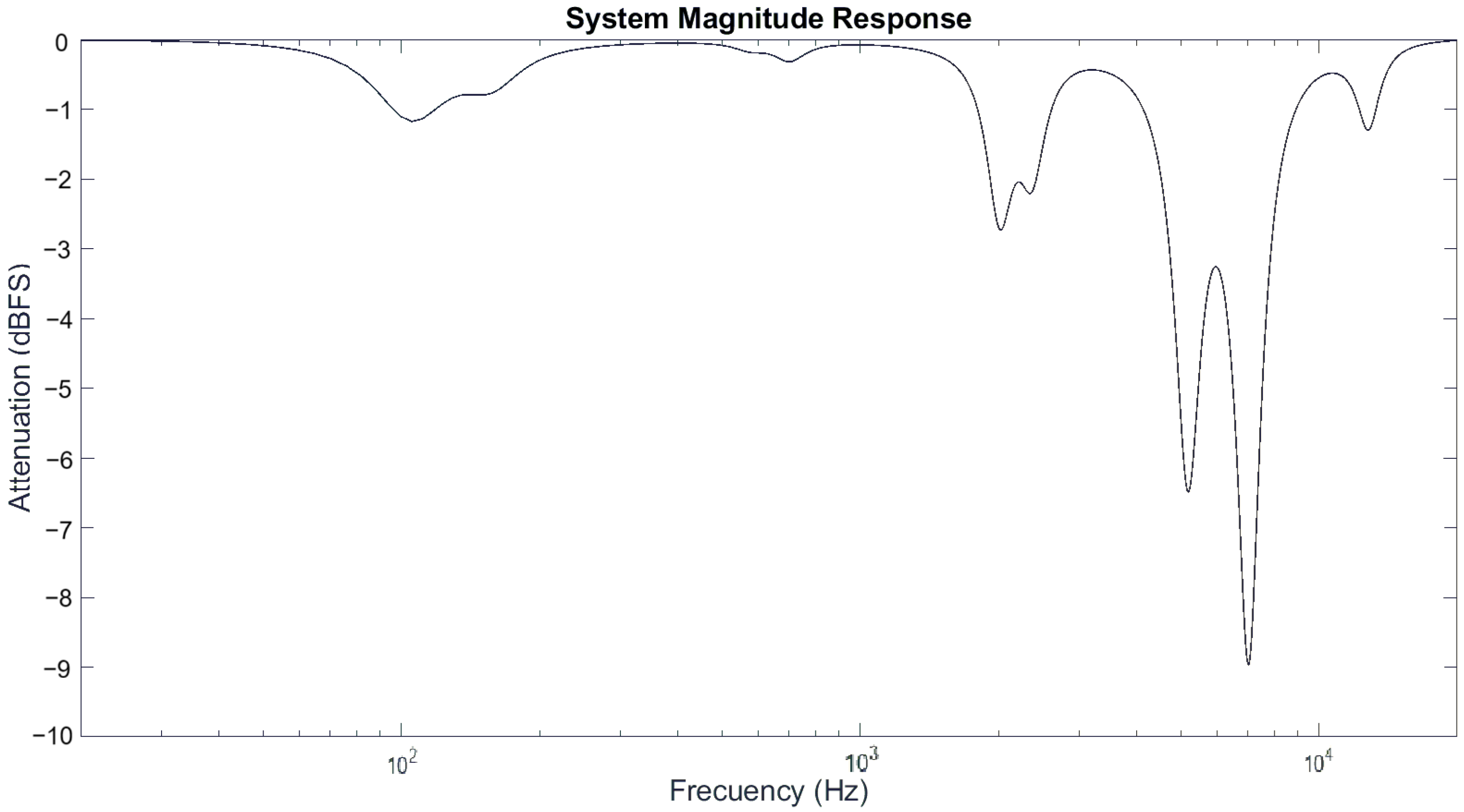
The transfer function is required for each filter, applied for each band. This results in the formation of a matrix of numerator and denominator coefficients. Table 1 contains a matrix that was generated from the analysis of an audio recording of a drum kit at a specific time instant. Its frequency response is shown in Figure 9.

Table 1.
Matrix generated from the analysis of an audio recording of a drum kit at a specific time instant.
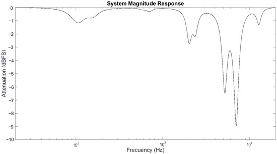
Figure 9.
System magnitude response for audio file of drum kit.
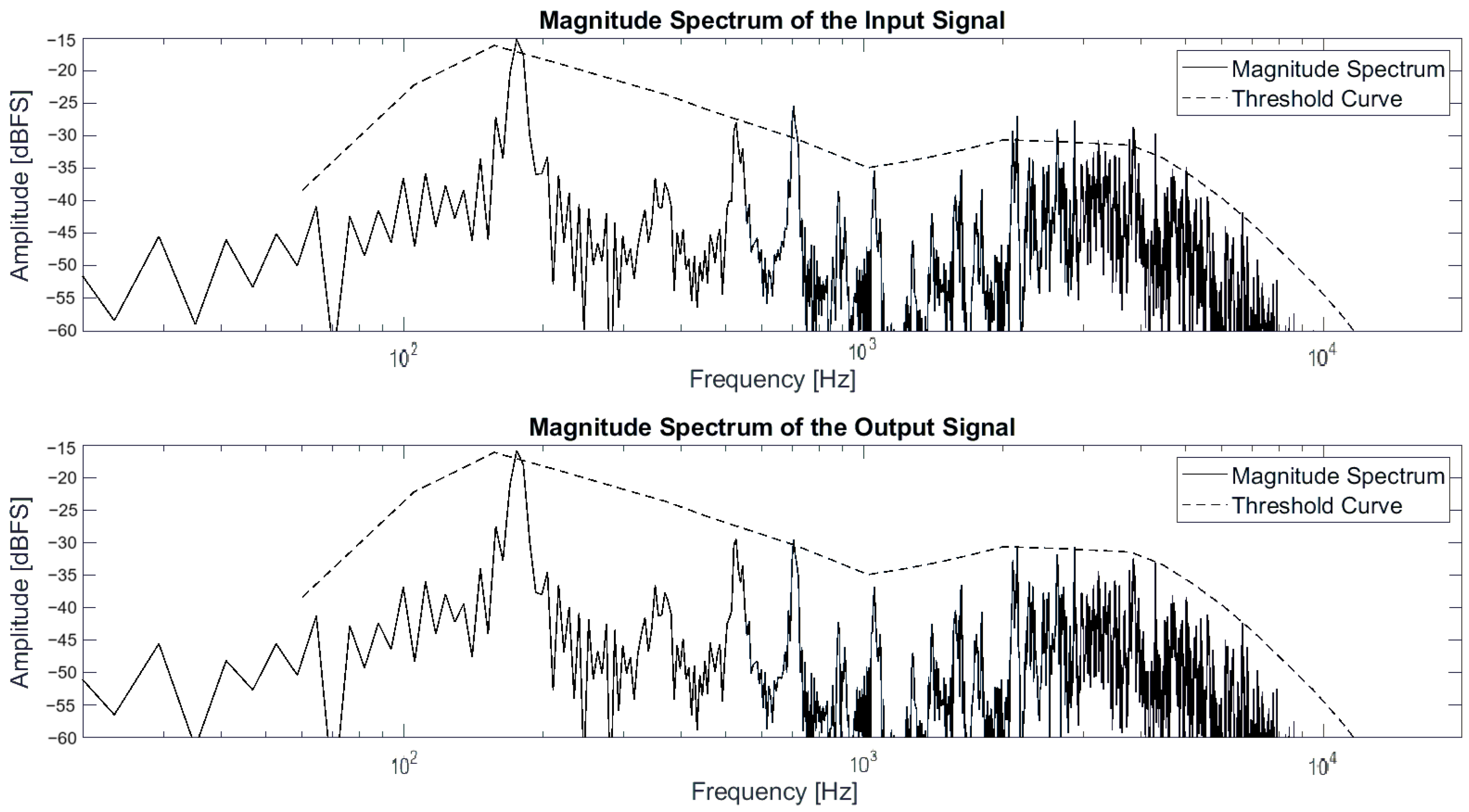
The matrix is then used to process the input signal, which is passed through a cascade of thirty second-order filters in order to process the entire spectrum by bands. In this study, the MATLAB DSP System Toolbox object dsp.SOSFilter was utilized for signal filtering, implementing an IIR filter structure with second-order sections. The default filtering structure is Direct form II transposed and the signal is filtered using the object, giving as arguments the input signal in matrix form (mono or stereo) and the coefficient matrix b corresponding to a 30 × 3 matrix and the coefficient matrix a corresponding to a 30 × 3 matrix. Finally, the output signal exhibits attenuation of the resonant frequencies across the entire spectrum. Figure 10 shows the magnitude spectrum of the input and output signal of a drum set file at a specific time together with the threshold curve.
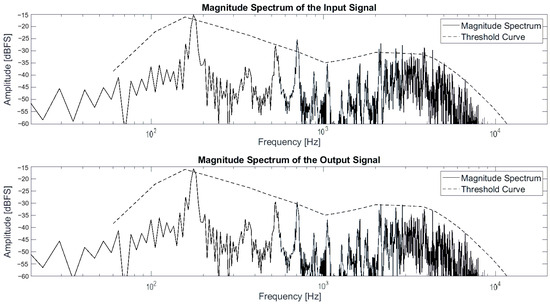
Figure 10.
Magnitude spectrum of input and output signal.
3. Results
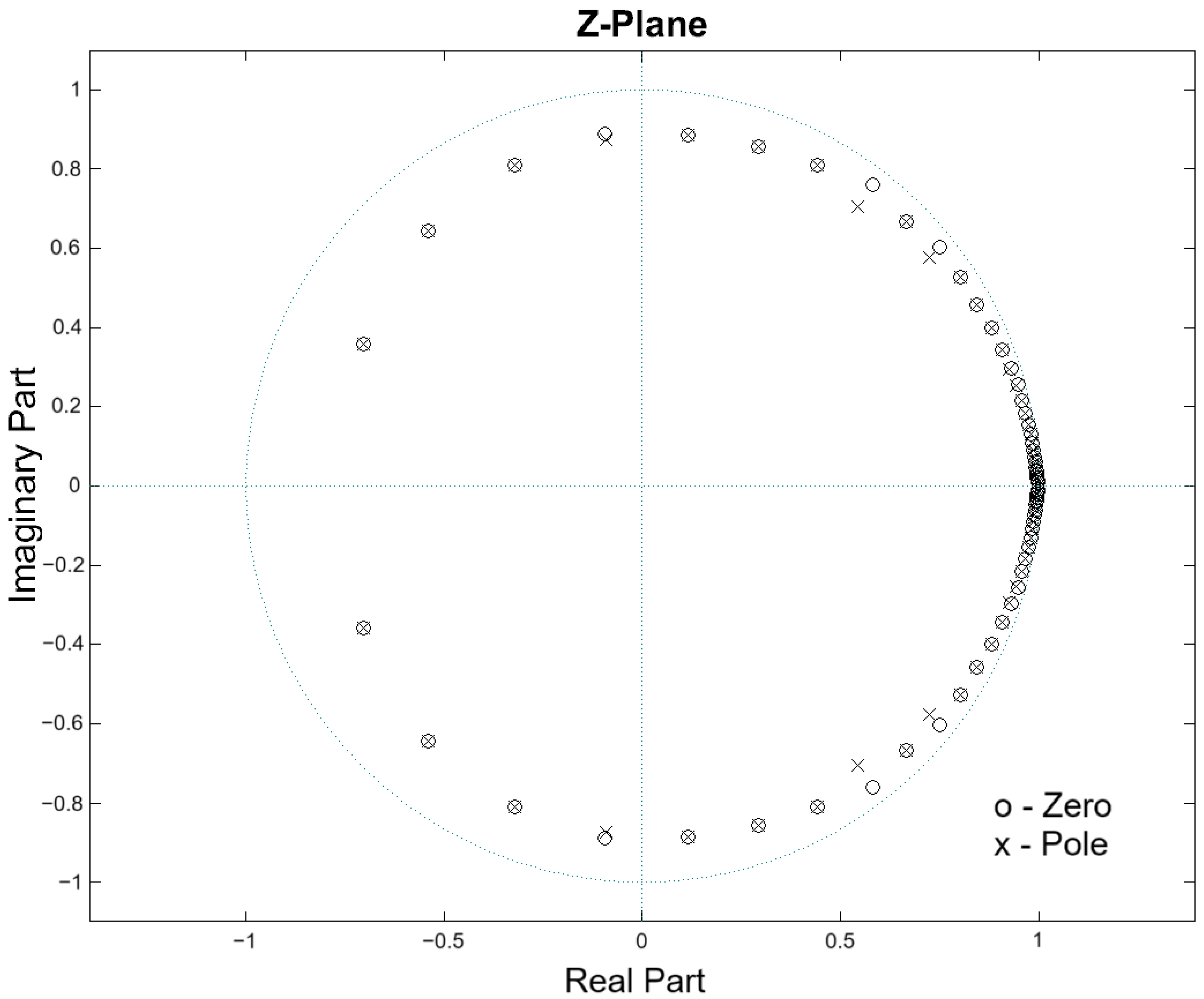
Pole-zero tests were conducted with the objective of identifying the conditions under which poles or zeros exited the unit circle. To achieve this, the operating frequency and attenuation variables of the second-order Peak IIR filter, as defined by Equation (10), were altered. A system becomes unstable when the poles are outside the unit circle, and it ceases to be of minimum phase when the zeros are outside the unit circle [19]. The stability of the system was probed under the Nyquist frequency, taking into consideration the maximum operating frequency of 22,000 Hz. This frequency is below the minimum audio frequency of 22,050 Hz (with a minimum sampling frequency of 44,100 Hz). Furthermore, the filter exhibits instability when the attenuation value is below −600 dBFS. To prevent this, the attenuation is constrained to a range of −145 dBFS to 0 dBFS. The preceding considerations indicate that the system will be stable and that the input signal will be processed with minimal delay, as all poles and zeros of the filter section are located within the unit circle. Figure 11 illustrates the pole-zero diagram for the Table 1 case and the frequency response of Figure 9 presented in Section 2.4.

Figure 11.
Unit circle in the Z-plane with poles and zeros at a specific time of the proposed system for audio from a drum set.
The algorithm’s performance was evaluated by developing it into an audio plug-in, enabling a direct comparison with the commercial plug-ins Soothe2 and RESO. The assessment was conducted using these plug-ins’ default settings and their free trial versions.
Twenty audio files from disparate sound sources were subjected to analysis and segmentation into five distinct groups. All these files can be found in the repository given at the end of this paper. The groups were designated as follows: percussion, guitars, wind instruments, other instruments, and voices. The dataset consists of twenty audio files that have been carefully selected to include a variety of instruments and conditions that are representative of real-life scenarios in commercial music applications. In particular, the selection includes versatile instruments in different conditions such as percussion with reverb, guitars in different scenarios such as acoustic, clean electric, distorted, and effects, vocals in different conditions, various wind instruments, and other instruments commonly used in commercial music such as the organ, piano, and electric bass. This diversity ensures that the dataset captures a wide range of acoustic characteristics. The metrics employed for analysis were the integrated RMS and LUFS levels measuring the attenuation of the processed audios. Attenuation by octave bands over time was obtained using the Wavelet transform.
Finally, the inter-annotator agreement metric was implemented with 40 individuals from the audio field involved in order to ascertain whether the attenuation generated was at resonant frequencies. The level of experience of the annotators ranged from 2 to 10 years or more in different areas of audio and music. Audio engineers, producers, musicians, audiophiles, and music-related people were considered in the evaluation. The experience of the annotators was carefully considered in order to ensure the transparency of the results for the project. In the course of the experiment, participants were asked to listen to the original audio files and to the audio files processed by the proposed plug-in, using headphones. After listening to each audio file, the participants were asked the following questions:
- Do you hear a difference between the output audio file and the input audio file?
- Do you consider the difference you hear in the output file to be the attenuation of resonant frequencies in the input audio file?
- Do you think the attenuation in the low/mid frequencies addresses the resonant frequencies of the input file?
- Do you think the attenuation in the mid/high frequencies addresses the resonant frequencies of the input file?
It should be noted that all four questions had only binary (yes/no) answers. From the responses, it was possible to average for each question how many people answered yes and how many answered no, thus analysing the responses across the spectrum and in low- and high-frequency sections.
In general, the developed plug-in exhibits higher attenuation than commercial plug-ins. As shown in Table 2, the attenuation is −2.32 dB in RMS and −2.33 in Integrated LUFS. In contrast, Soothe2 has an attenuation of −1.27 dB in RMS and −1.28 Integrated LUFS. RESO exhibits an attenuation of −1.1 dB in RMS and −1.08 Integrated LUFS.
Table 2.
RMS and Integrated LUFS values for the three analyzed plug-ins.
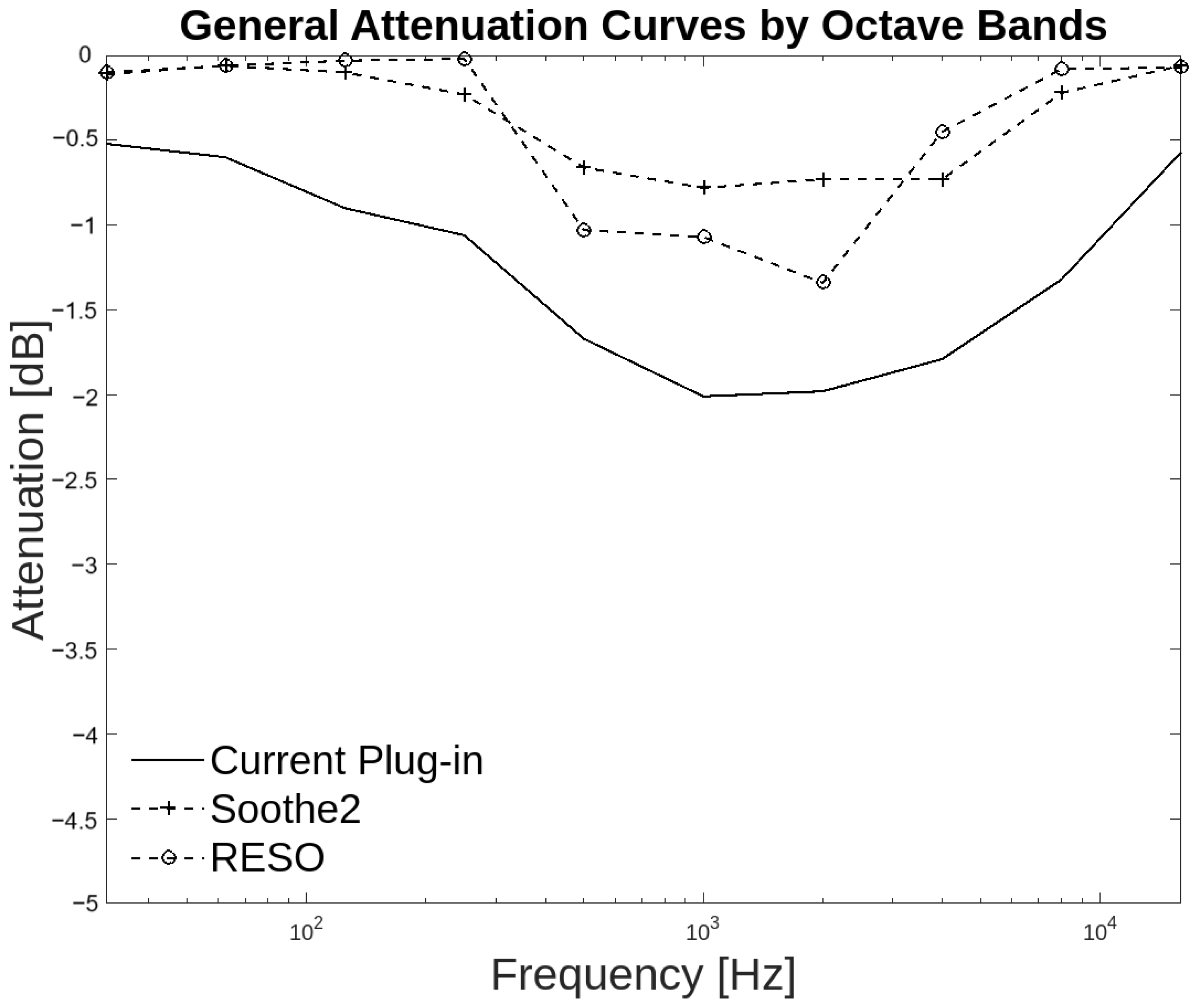
The present study employs a statistical approach based on octave bands and by groups of audio files instead of analyzing specific resonant frequencies in each piece of audio. This method allows more general conclusions to be drawn about the effectiveness of the system in the proposed groups while avoiding biases caused by individual cases. The octave band analysis revealed that, in terms of attenuation, the audio plug-in generally coincided with the other two plug-ins in the 31.25 Hz band and from 500 Hz to 4 kHz. There was a notable degree of agreement between the present work and Soothe2, with both 125 Hz and 8 kHz exhibiting attenuation greater than −0.1 dB, as illustrated in Table 3 and Figure 12.
Table 3.
Average attenuation per octave band of all audio files in dBFS.
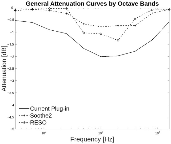
Figure 12.
General attenuation curves by octave bands for three plug-ins.
In the analysis of the annotator agreement, 74% of the population indicated that attenuation occurs at the resonant frequencies throughout the spectrum. Additionally, 59% of respondents agreed that attenuation in low frequencies occurs at the resonances, while 60% of respondents agreed that attenuation of high frequencies occurs at the resonances in that section.
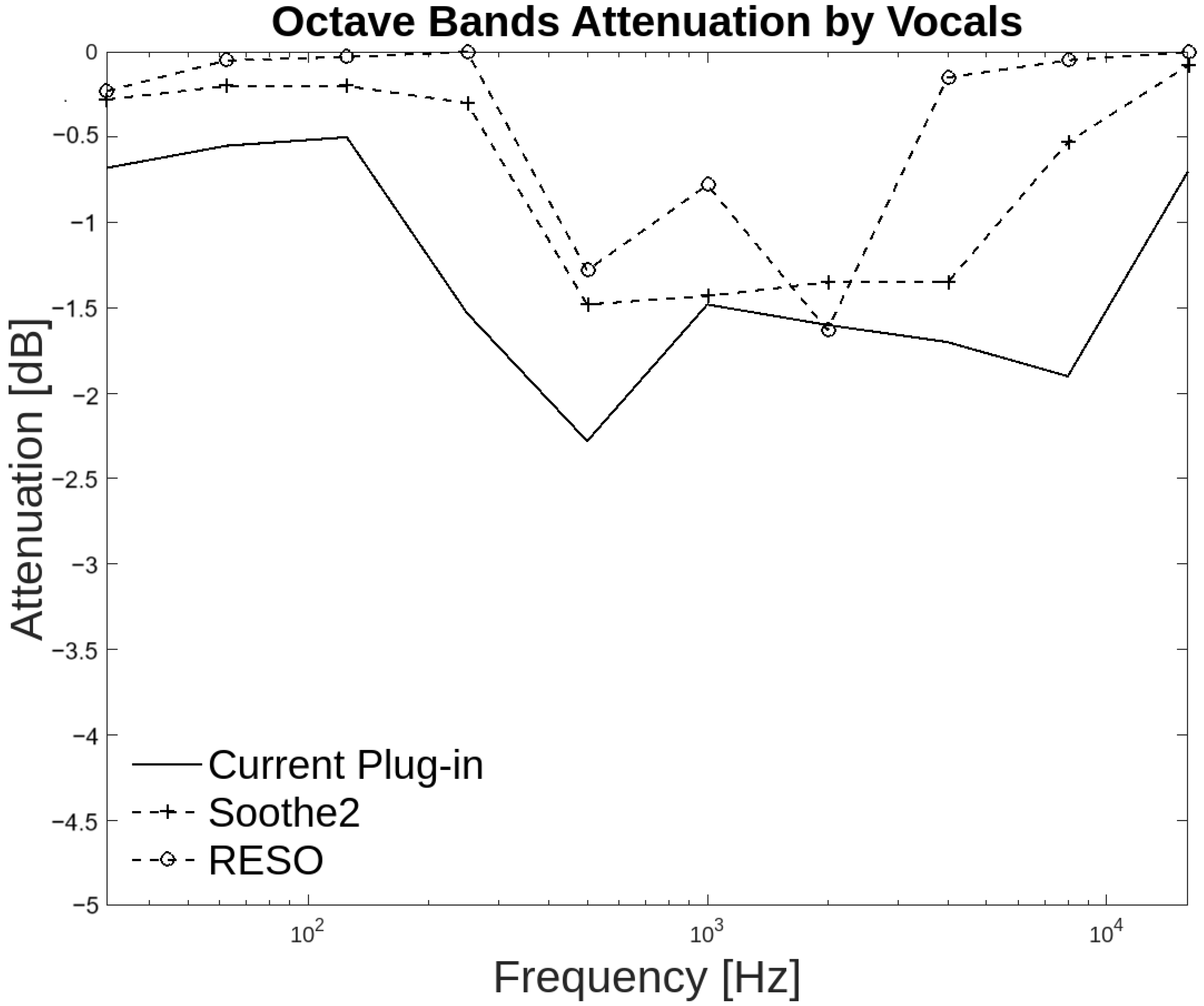
Additionally, each group of audio files was analyzed by octave bands. The group where there is a general agreement between the three plug-ins is the voice group. In this group, the three plug-ins agree at 31.25 Hz and from 500 Hz to 4 kHz with attenuation between −2.5 dB and −1 dB. With Soothe2, the agreement extends from 31.25 Hz to 8 kHz. The Figure 13 illustrates that the three plug-ins generate comparable attenuation. It can be confirmed that the attenuation occurs over the resonant frequencies, as evidenced by the 83.75% of respondents who indicated that the attenuation occurs over the resonant frequencies in the annotator agreement. Additionally, 66.25% of respondents indicated that the attenuation occurs over high frequencies coinciding with the resonant frequencies. These frequencies are crucial because they contain the highest harmonic content of voices.

Figure 13.
Octave band attenuation curves for the three plug-ins in the voice group.
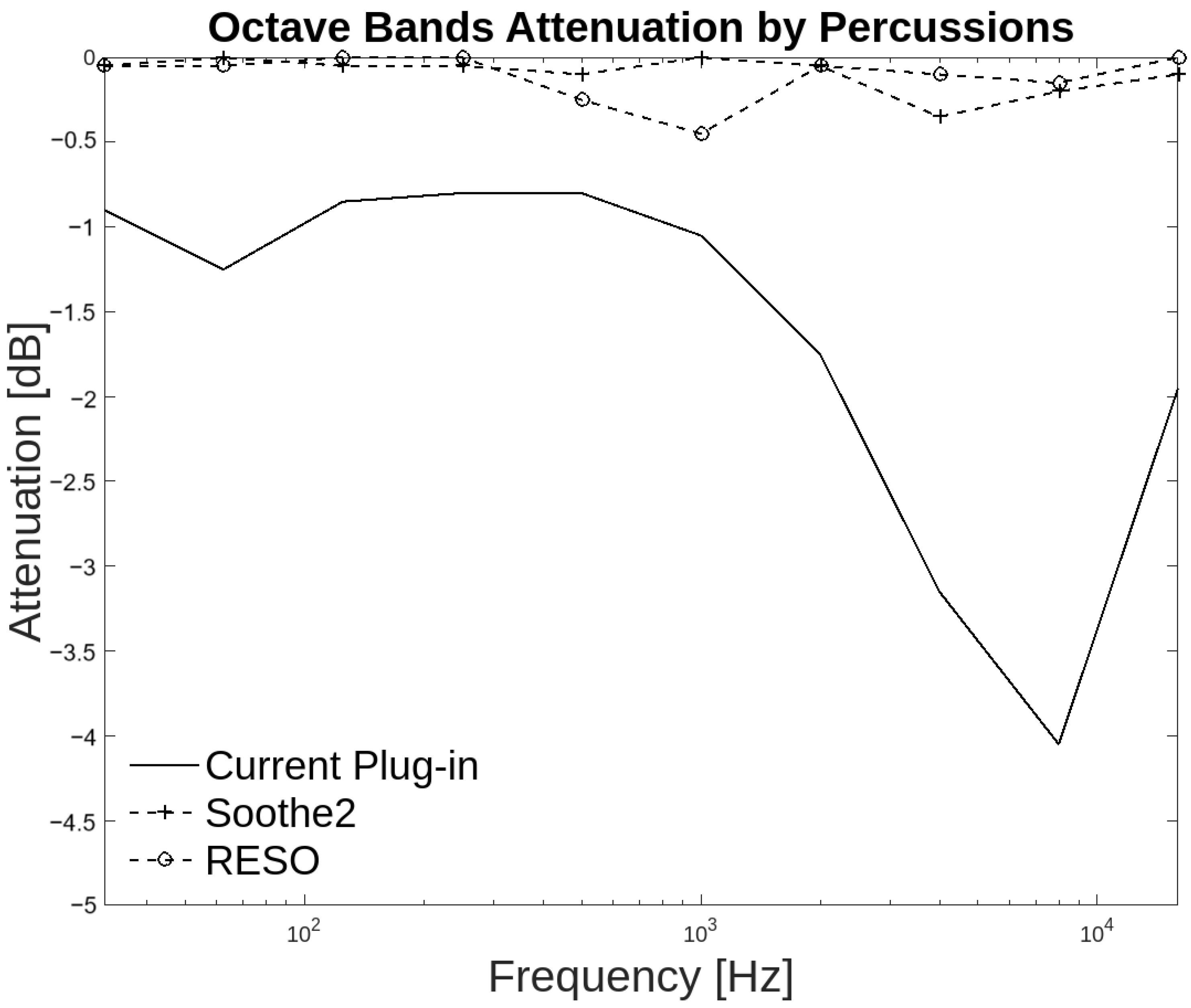
The developed plug-in exhibits greater attenuation than the other two in the percussion and guitar groups. In percussion instruments, the plug-in produces a higher attenuation of −0.5 dB from 31.25 Hz to 250 Hz, while Soothe2 and RESO generate attenuation of less than −0.5 dB, as illustrated in the Figure 14. The low frequencies present in percussion instruments are of significant importance, as these instruments encompass the entire auditory spectrum and possess a high low-frequency content.

Figure 14.
Octave band attenuation curves for the three plug-ins in the percussion group.
All three plug-ins exhibit attenuation exceeding −0.1 dB at frequencies of 500 Hz, 4 kHz, and 8 kHz. However, it should be noted that the proposed plug-in generates −3.5 dB more than commercial plug-ins at the 8 kHz frequency.
A total of 65% of respondents indicated that attenuation at low frequencies occurs at the resonant frequencies. Similarly, 67.5% of respondents agreed that attenuation of high frequencies occurs at the resonances. These results indicate that attenuation across the spectrum occurs at the resonances of the percussion instruments.
In the guitar group, the plug-ins match attenuation values greater than −0.1 dB from 500 Hz to 8 kHz. With Soothe2, attenuation values match from 125 Hz to 8 kHz. The plug-in of the present work matches RESO from 500 Hz to 16 kHz with attenuation values up to −2.6 dB, as shown in Figure 15. A guitar has spectral content from 82 Hz to 15 kHz, which coincides with the region that the present work attenuates. In the annotators’ agreement, 65% of people agreed that the attenuation at high frequencies was above the resonant frequencies. The high frequencies are important since guitars have high harmonic content in this region.
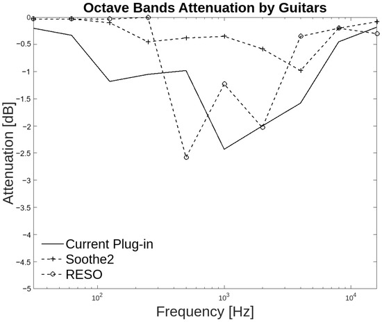
Figure 15.
Octave band attenuation curves for the three plug-ins in the guitar group.
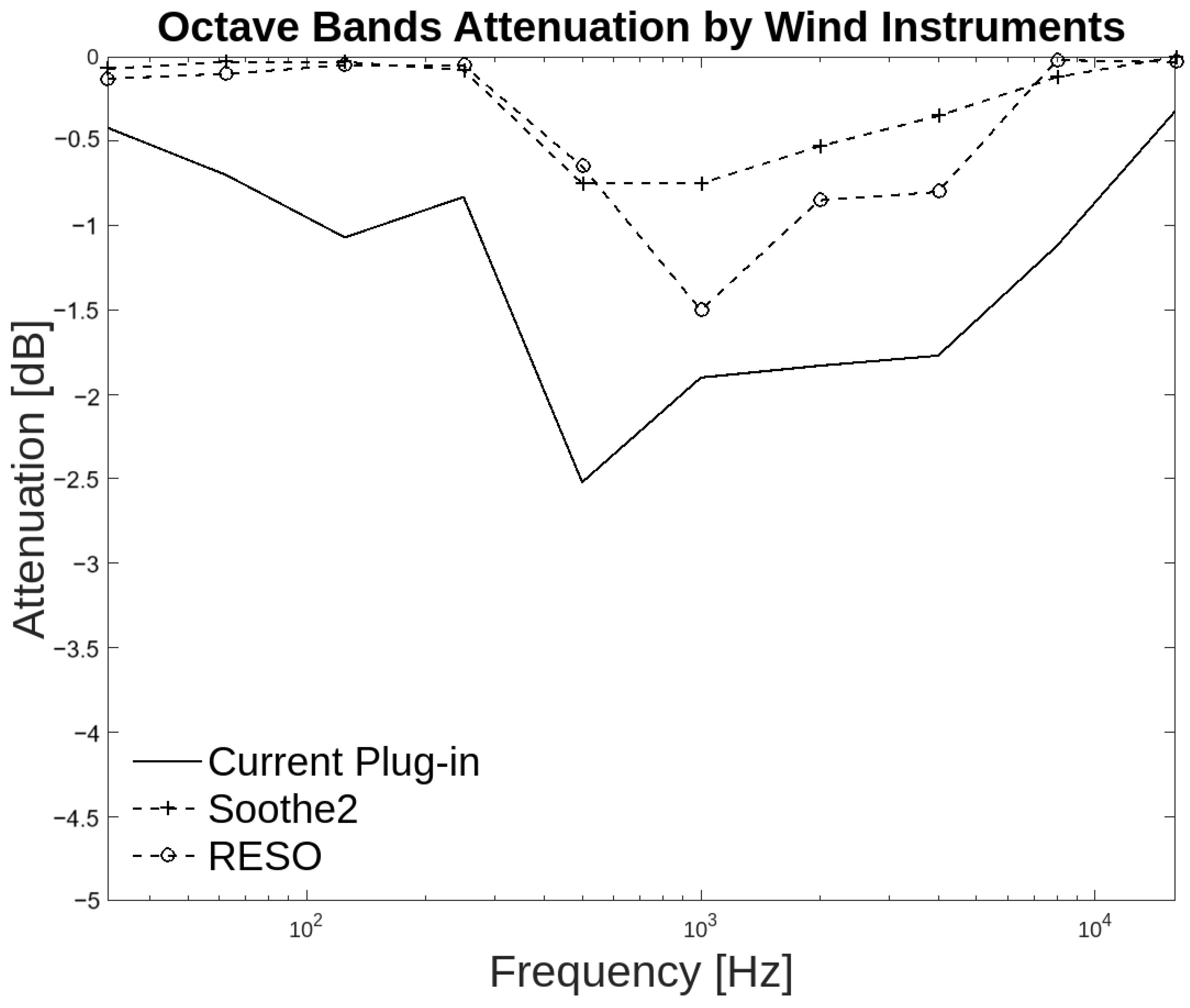
In the wind and other instrument groups, despite the proposed plug-in having higher attenuation than the commercial plug-ins in the annotator agreement, there is a discrepancy. The three plug-ins in the two groups matched from 500 Hz to 4 kHz with similar attenuation curves, although the proposed plug-in generates higher attenuation. Wind instruments have different ranges depending on each instrument. Some instruments have mid/high frequency content, while others have mid/low frequency content. As shown in Figure 16 the plug-in generates attenuation from 125 Hz to 250 Hz, which helps to control resonances at fundamental frequencies of these instruments.
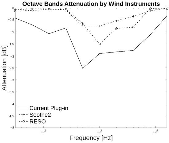
Figure 16.
Octave band attenuation curves for the three plug-ins in the wind instruments group.
The annotators of this group reached a consensus in which 60.83% of people agreed that the attenuation in low frequencies was above the resonant frequencies. However, in the high frequencies, only 52.5% considered that the attenuation occurred over the resonant frequencies. This discrepancy may be attributed to the different harmonic content of wind instruments, whereby in some cases the low frequencies are more present than the high frequencies.
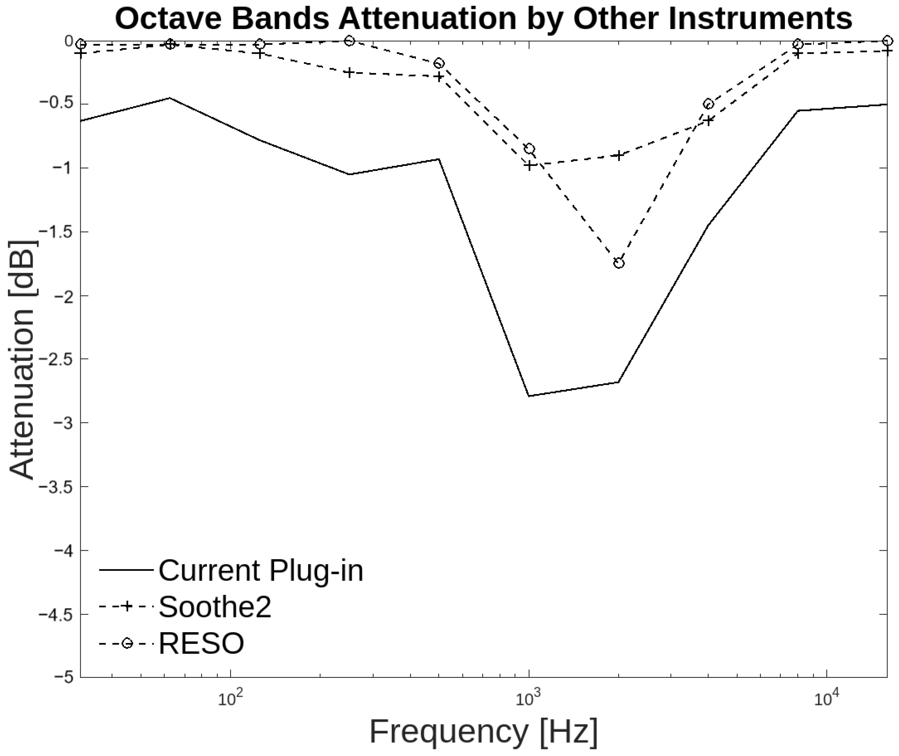
A similar phenomenon occurs with the group of other instruments. Each instrument has a distinct frequency range. Each instrument is situated within a specific range, and for the listener, it can be challenging to perceive the ranges. This is evident in the results of the inter-annotator agreement, as 53.75% of respondents indicated that attenuation occurred for the resonances in low frequencies, while 56.25% of respondents believed that the attenuation of high frequencies occurred at the resonant frequencies. The highest attenuation value generated by the plug-in in this group is −2.8 dB, as illustrated in Figure 17. There is a higher degree of correlation with the Soothe2 plug-in in eight bands, which are at 31.25 Hz and from 125 Hz up to 8 kHz.
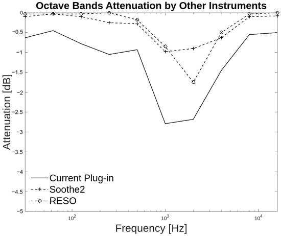
Figure 17.
Octave band attenuation curves for the three plug-ins in the group of other instruments.
This analysis reveals that the design of the developed work is analogous to that of Soothe2, as evidenced by the concurrence of attenuation curves in frequency zones and the degree of attenuation. While the developed plug-in exhibits a greater degree of attenuation in specific frequency sections, the attenuation levels across all bands are comparable. This is attributed to the operational principles of the developed plug-in, which differ from those of RESO.
4. Conclusions
The analysis of a greater number of samples in the frequency domain allows for greater precision in the analysis of low frequencies. The plug-in of the present work demonstrates superior performance at these frequencies, as evidenced by the tests conducted on audio samples belonging to the percussion group. This is due to the fact that the plug-in in question generates attenuation at frequencies below 250 Hz, with attenuation values ranging from −0.8 dB to −1.25 dB. In contrast, the attenuation generated by Soothe2 and RESO is close to 0 dB.
The algorithm generates a curve using the standard deviation rule of thumb and linear interpolation functions as a threshold curve for detecting resonant frequencies. This is because the peaks of the signal are neglected, resulting in a general shape of the spectrum. The energy accumulation is higher in specific areas, which can be observed in this curve.
The utilization of octave band-based analysis enables the estimation of resonance attenuation without the necessity of identifying each specific resonant frequency. Matching the detection zones with commercial tools such as Soothe2 confirms that the algorithm adequately captures the resonance patterns.
This similarity is due to the fact that the architecture of Soothe2 is similar to that of the algorithm. The present work and Soothe2 employ a dynamic filter approach, continuously analyzing the signal and proposing filters based on the buffer size. This contrasts with RESO, which analyzes a fixed section of the audio and proposes static filters for the entire audio.
The second-order filter section processes the signal with minimum and stable phase filters. This is due to the amplitude and frequency considerations made, which ensure that the poles and zeros of the filter remain within the unit circle of the Z-plane.
In the comparison of the developed system with commercial plug-ins, the attenuation generated by the developed system was found to be higher. The average attenuation generated by the plug-in was found to be adequate, as an intermediate point of attenuation between 0 dB and 6 dB is required. This is because attenuation higher than −0.25 dB is barely perceptible to the human ear, while attenuation lower than −6 dB reduces sound perception by half. The attenuation falls within the specified range and is also higher than that of the other two commercial plug-ins.
The attenuation zone where there is agreement between the three systems is from 500 Hz to 4 kHz. Based on the equal loudness curves, the 4 kHz zone is of particular importance because it is the most sensitive to the human ear.
A system was thus developed to detect and attenuate resonant frequencies in audio files, with satisfactory results. The plug-in performs optimally on audio signals originating from voices and instruments such as drums and guitars. In other audio signals, such as those originating from wind or other instruments, the proposed plug-in attenuates more than other commercial plug-ins, yet it does not ensure that the attenuation occurs over resonant frequencies.
Frequency band-based analysis proves to be a valid strategy to evaluate the effectiveness of a system without the need to identify individual resonant frequencies. Since energy build-up in certain bands is a reliable indicator of problematic resonances, this approach allows conclusions to be drawn on groups of audios in a general way.
Given our development of an actual plug-in in VST format, it is possible to implement our work in any DAW or system that reads this format. This enables the processing of audio files for various applications, including production, mixing, and mastering of music, as well as voice in movies, podcasts, and radio. Additionally, some digital mixers provide support for this format, which can be utilized to eliminate feedback and adjust audio levels in live sound.
Author Contributions
Conceptualization, D.U.-H., J.P.F.P.-D., F.J.G.-F., A.J.R.-S., E.V.-L., A.A.M.-G. and L.C.-S.; investigation, D.U.-H., J.P.F.P.-D., F.J.G.-F., A.J.R.-S., E.V.-L., A.A.M.-G. and L.C.-S.; methodology, D.U.-H., J.P.F.P.-D., F.J.G.-F., A.J.R.-S. and A.A.M.-G.; project administration, D.U.-H., J.P.F.P.-D., F.J.G.-F., A.J.R.-S., E.V.-L., A.A.M.-G. and L.C.-S.; software, D.U.-H., J.P.F.P.-D. and F.J.G.-F.; supervision, D.U.-H., J.P.F.P.-D., F.J.G.-F., A.J.R.-S., E.V.-L., A.A.M.-G. and L.C.-S.; validation, D.U.-H., J.P.F.P.-D., F.J.G.-F., A.J.R.-S., E.V.-L., A.A.M.-G. and L.C.-S.; writing—original draft, D.U.-H., J.P.F.P.-D. and F.J.G.-F.; writing—review and editing, D.U.-H., J.P.F.P.-D., F.J.G.-F., A.J.R.-S., E.V.-L., A.A.M.-G. and L.C.-S. All authors have read and agreed to the published version of the manuscript.
Funding
This research received no external funding.
Institutional Review Board Statement
Not applicable.
Informed Consent Statement
Not applicable.
Data Availability Statement
The processed files can be found at the following link: https://zenodo.org/doi/10.5281/zenodo.12802627.
Acknowledgments
The authors thank the Instituto Politécnico Nacional and Consejo Nacional de Humanidades Ciencias y Tecnologías for their support in carrying out the work of this research.
Conflicts of Interest
The authors declare no conflict of interest.
Abbreviations
The following abbreviations are used in this manuscript:
| FFT | Fast Fourier Transform |
| RMS | Root Mean Square |
| LUFS | Loudness Units Full Scale |
| VST | Virtual Studio Technology |
| DAW | Digital Audio Workstation |
| ERB | Equivalent Rectangular Bandwith |
References
- Välimäki, V.; Reiss, J.D. All About Audio Equalization: Solutions and Frontiers. Appl. Sci. 2016, 6, 129. [Google Scholar] [CrossRef]
- Martignon, P.; Ponteggia, D.; Di Cola, M. Measurement Techniques for Dynamic Equalizers. In Proceedings of the Audio Engineering Society Convention 155, Audio Engineering Society, New York, NY, USA, 25–27 October 2023. [Google Scholar]
- Wilmering, T.; Moffat, D.; Milo, A.; Sandler, M.B. A History of Audio Effects. Appl. Sci. 2020, 10, 791. [Google Scholar] [CrossRef]
- Bitzer, J.; LeBoeuf, J.; Simmer, U. Evaluating Perception of Salient Frequencies: Do Mixing Engineers Hear the Same Thing? In Proceedings of the Audio Engineering Society Convention 124, Amsterdam, The Netherlands, 17–20 May 2008. [Google Scholar]
- Liski, J. Equalizer Design for Sound Reproduction. Ph.D. Thesis, Aalto University, Espoo, Finland, 2020. [Google Scholar]
- Ballou, G. Handbook for Sound Engineers; Taylor & Francis: Oxford, UK, 2015. [Google Scholar]
- Oeksound. Soothe2 Manual. Oeksound. 2024. Available online: https://oeksound.com/manuals/soothe2/ (accessed on 3 May 2024).
- Mastering the Mix. RESO Manual. Mastering the Mix. 2024. Available online: https://www.masteringthemix.com/pages/reso-manual (accessed on 4 May 2024).
- Corbach, T.; von dem Knesebeck, A.; Dempwolf, K.; Holters, M.; Sorowka, P.; Zölzer, U. Automated equalization for room resonance suppression. In Proceedings of the 12th International Conference Digital Audio Effects (DAFx09), Como, Italy, 1–4 September 2009. [Google Scholar]
- Wakefield, J.; Dewey, C. Evaluation of an algorithm for the automatic detection of salient frequencies in individual tracks of multitrack musical recordings. In Proceedings of the Audio Engineering Society Convention 138, Audio Engineering Society, Warsaw, Poland, 7–10 May 2015. [Google Scholar]
- Bitzer, J.; LeBoeuf, J. Automatic detection of salient frequencies. In Proceedings of the Audio Engineering Society Convention 126, Audio Engineering Society, Munich, Germany, 7–10 May 2009. [Google Scholar]
- Presti, G.; Degiorgi, N.; Fresia, A.; Servetti, A. Real-time psychoacoustic frequency masking compensation for audio signals with overlapping spectra. In Proceedings of the 21st Sound and Music Computing Conference, Porto, Portugal, 4–6 July 2024. [Google Scholar]
- Posada Hernández, G.J. Elementos básicos de Estadística Descriptiva Para el Análisis de Datos; Fondo Editorial Luis Amigó: Medellin, Colombia, 2016. [Google Scholar]
- de San Buenaventura, U. Cambios de Nivel. 2017. Available online: https://matdiaz.github.io/index.html (accessed on 15 May 2024).
- Basso, G. Percepción Auditiva; Universidad Nacional de Quilmes Editorial: Buenos Aires, Argentina, 2018. [Google Scholar]
- 11-1986, A.S; Specification for Octave-Band and Fraction-Octave-Band Analog and Digital Filters. American National Standards Institute: Washington, DC, USA, 1986.
- Abdallah, A.B.; Hajaiej, Z. Improved closed set text independent speaker identification system using Gammachirp Filterbank in noisy environments. In Proceedings of the 2014 IEEE 11th International Multi-Conference on Systems, Signals & Devices (SSD14), Castelldefels-Barcelona, Spain, 1–14 February 2014; pp. 1–5. [Google Scholar]
- Peeters, G. A large set of audio features for sound description (similarity and classification) in the CUIDADO project. (CUIDADO) Ist Proj. Rep. 2004, 54, 1–25. [Google Scholar]
- Socoró, J.C.; Morán Moreno, J.A. Diseño de filtros discretos. Proceso avanzado, febrero 2014. Uoc Learn. Resour. 2014, 1, 1–84. [Google Scholar]


Disclaimer/Publisher’s Note: The statements, opinions and data contained in all publications are solely those of the individual author(s) and contributor(s) and not of MDPI and/or the editor(s). MDPI and/or the editor(s) disclaim responsibility for any injury to people or property resulting from any ideas, methods, instructions or products referred to in the content. |
© 2025 by the authors. Licensee MDPI, Basel, Switzerland. This article is an open access article distributed under the terms and conditions of the Creative Commons Attribution (CC BY) license (https://creativecommons.org/licenses/by/4.0/).