The Seismic Dynamic Response Characteristics of the Steep Bedding Rock Slope Are Investigated Using the Hilbert–Huang Transform and Marginal Spectrum Theory

Abstract

The steep bedding rock slope (SBRS) is easily destabilized under earthquake action, so it is crucial to research the features of this kind of slope’s seismic dynamic reactions in order to prevent and mitigate disasters. Few researchers have examined these slopes from an energy perspective, and the majority of recent research focuses on the displacement and acceleration response patterns of these kinds of slopes under seismic action. This work performed an extended study of a dynamic numerical simulation and systematically analyzed the dynamic response characteristics of this type of slope under earth quake conditions from the standpoint of energy utilizing the Hilbert–Huang transform (HHT) and marginal spectrum (MSP) theory. This was carried out in response to the slope’s shaking table test from our previous work. The findings indicate the following: (1) The ‘elevation effect’ and ‘surface effect’ are clearly seen in the acceleration amplification factor (AAF) of the slope during an earthquake. The selectivity of the slope acceleration’s Fourier spectrum amplification impact indicates that the elevation amplification effect makes the high-frequency peak’s amplitude more noticeable. (2) Although the effect of the weak layer is more pronounced in the high-frequency portion, both the elevation and the weak layer affect the seismic wave’s Hilbert energy. As a result, the weak layer at the top of the slope is usually destroyed first during an earthquake. (3) Prior to the locked segment’s penetration failure at the toe of the SBRS, the Hilbert energy of the high-frequency band of the marginal spectrum at the monitoring point on the top portion of the segment will rise sharply. This suggests that the upper portion of the locked segment has begun to sustain damage. There are antecedents even when there is no penetration failure.

1. Introduction

Due to its significant seismic activity, numerous slopes, and delicate geological environment, southwest China is particularly vulnerable to instability during seismic activity. [1,2,3]. A common type of slope in this region is the steep bedding rock slope. When instability arises during an earthquake, it frequently results in significant damage, which presents a significant hidden risk to the security of nearby infrastructure as well as the lives and property of local residents [4,5]. There have been tens of thousands of landslide disasters since the 2008 Wenchuan earthquake. The SBRS caused significant damage at the time, including the Dazhuping landslide in Gaochuan Township, the Tangjiashan landslide in Beichuan County, and the Qianfoyan Ganmofang landslide in Anxian County [6,7,8,9]. For instance, the safety of 300,000 people downstream of Miayang City was seriously threatened by the Tangjiashan landslide, which produced the greatest weir following the Wenchuan earthquake [10]. Therefore, studying the dynamic response and failure mode of the SBRS under earthquake activity is extremely important from both a theoretical and practical standpoint.

At present, the primary technical tools for analyzing the dynamic response and failure mode of the SBRS under earthquake action are numerical simulations and the shaking table test [11,12,13,14]. Wang et al. [15] used a numerical simulation to examine the collapse process of an SBRS and suggested that the primary cause of this kind of landslide’s instability was the weakening of the internal layer. Using a numerical simulation and shaking table model testing, Xin et al. [16] discovered that when seismic activity occurs, the acceleration close to the weak surface increases suddenly, creating a lot of secondary cracks before the weak surface changes into a sliding surface. Through a numerical simulation, Tan et al. [17] discovered that the weak surface significantly impacted the bedding slope’s shear failure process, exhibiting clear nonlinear deformation and tensile shear failure characteristics. Shaking table studies on bedding rock slopes and clastic rock slopes were performed by Wang et al. [18]. They discovered that the accumulation layer on the slope surface amplifies seismic waves and can lead to slope failure. By using a shaking table model test to replicate the progressive failure process of the SBRS, Zang et al. [19] suggested that the weak surface was a major factor in the deformation and failure of bedding rock slopes. This provided a plausible explanation for the widespread shallow rock slope sliding that occurs during earthquake activity. Dong et al. [20] conducted a shaking table test. Tensile-shear sliding failure was identified as the SBRS’s failure mode after an analysis of the slope’s acceleration, displacement, and acoustic emission response under various seismic wave frequencies.

Note that while the majority of the aforementioned studies concentrate on the failure mode and acceleration amplification effect of the SBRS under seismic activity, there is still a lack of thorough research on the seismic energy within the slope. In fact, seismic energy is the key trigger factor for dynamic failure of slopes. Analyzing the slope’s dynamic response and failure mode from an energy perspective is crucial [21]. The most widely utilized analytical techniques for efficiently determining the energy distribution of seismic signals in the time–frequency domain are the Hilbert–Huang transform and marginal spectrum theory. Previous researchers have used this method to study the dynamic response law of slopes [22]. An energy-based approach based on the HHT and MSP theory was put forth by Fan et al. [23] to analyze the dynamics of landslides caused by earthquakes. Based on the HHT and the MSP theory, Song et al. [24,25] discovered that the HHT and the MSP, respectively, can represent the slope’s overall deformation and local deformation. They also clarified the slope’s dynamic damage process from an energy perspective. Large-scale shaking table tests were conducted by Chen et al. [26]. Through HHT, it was discovered that one of the main causes of slope failure was the variation in instantaneous frequency energy distribution characteristics in various stages of the process. Lei et al. [27] found that low-frequency energy has a substantial influence on the bottom portion of the slope, whereas high-frequency energy has a significant impact on the upper, central part of the slope through the trend in marginal spectral shifts. In conclusion, thorough studies on the dynamic response law of the SBRS using this approach are still absent, despite the fact that the HHT and the MSP theory have been employed to examine the seismic dynamic response of slopes.

This study uses the SBRS as its research object, builds on numerical simulation research based on the slope shaking table test conducted earlier, explores its dynamic response characteristics using the HHT and MSP theory, examines the amplitude of seismic waves and the impact of the weak layer on the slope’s dynamic response, and then re-reveals the dynamic response of the SBRS from an energy perspective. Lastly, the energy point of view is used to demonstrate the dynamic reaction of the SBRS. The findings of this study may offer some recommendations for catastrophe mitigation and preventive initiatives in seismically active regions.

2. Numerical Simulation Scheme

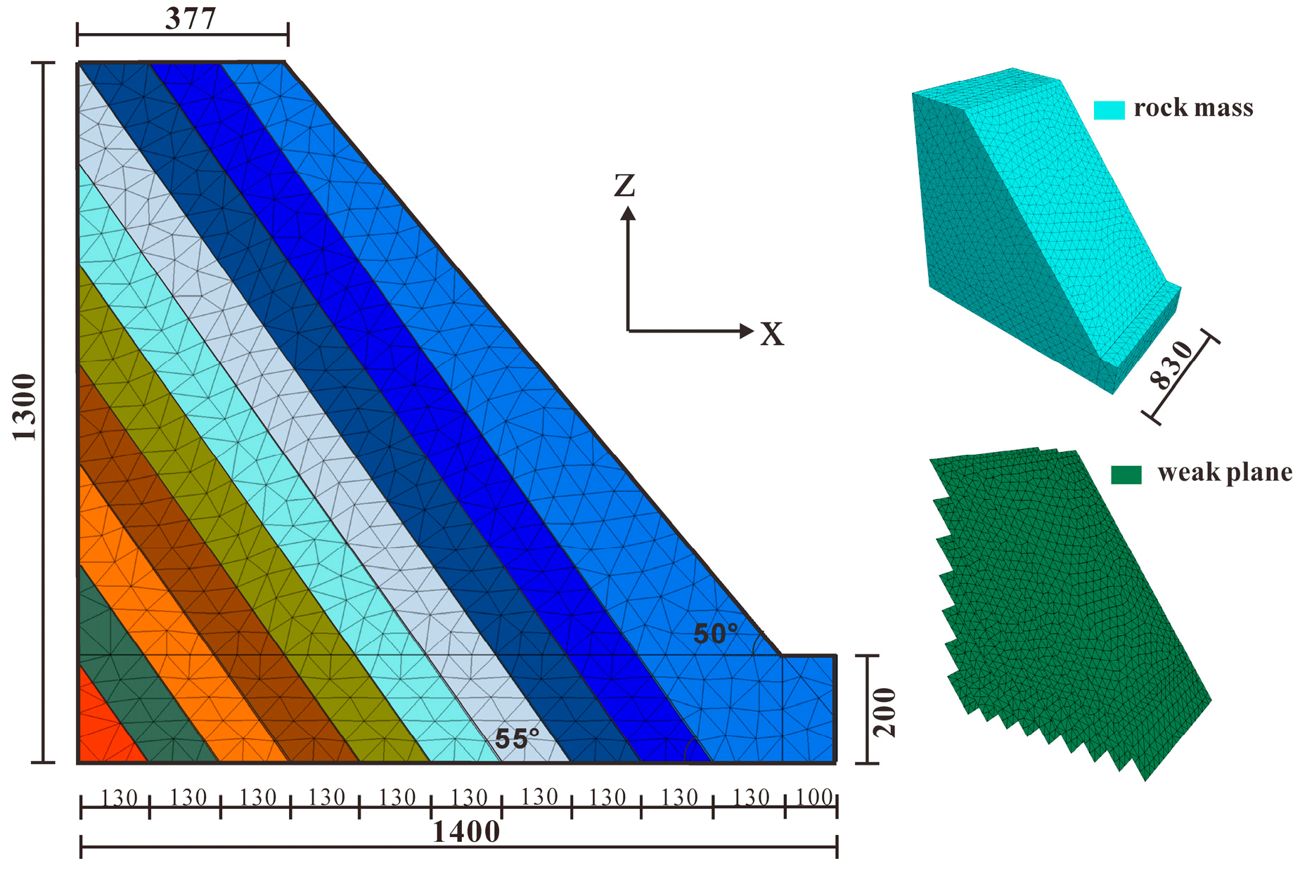
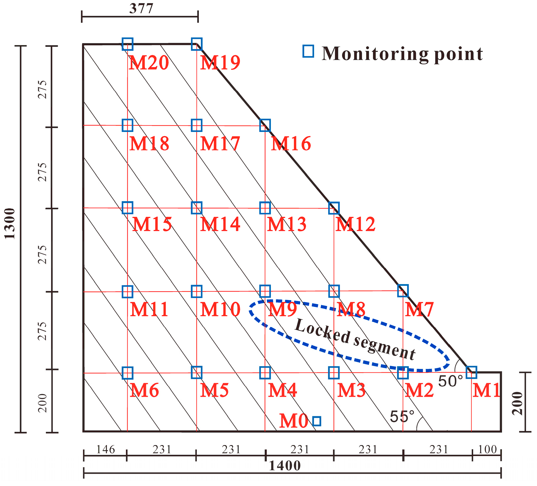
2.1. Establishing the Numerical Model

Using discrete element 3DEC software (3.0 version), a numerical model of the SBRS of the same size was created based on our earlier shaking table test [20] (Figure 1 and Figure 2). The dynamic response and damage mechanisms of the slope under seismic action were thus analyzed through the extension of numerical simulation. The slope model’s precise dimensions are 140 cm for length, 83 cm for width, and 130 cm for height. Its slope angle is 50°, its horizontal distance from the rock layer is 13 cm, its dip angle is 55°, and a mica sheet is placed in between the layers. It should be noted that when using numerical simulation for seismic conditions, in order to meet the simulation accuracy requirements, the mesh size Δl follows the rule proposed by Kuhlemeyer and Lysmer [28], which is estimated as follows:

$$\Delta l\le {\displaystyle \frac{\lambda }{10}} \sim {\displaystyle \frac{\lambda }{8}},$$

(1)

where Δl is the mesh size, and λ is the wavelength corresponding to the highest component frequency of the input wave. Accordingly, we set the mesh size to 0.05 m to ensure the complete propagation of seismic waves in the medium, and the final delineation model contains a total of 13,723 grid nodes and 50,198 mesh elements (Figure 2).

The Mohr–Coulomb yield criteria was employed for analysis, and the plastic constitutive model was used for the rock mass in the numerical model of the slope.

Table 1. Physical–mechanical parameters in numerical model of the slope. (a) Physical and mechanical parameters of rock mass. (b) Physical and mechanical parameters of weak layer.

(a)
Item	Density (g/cm3)	Young Modulus (MPa)	Poisson Ratio	Friction Angle (°)	Cohesion (kPa)
Rock mass	2.50	124.46	0.12	34.8	294.0
(b)
Item	Stiffness—Normal (Pa)		Stiffness—Shear (Pa)	Friction Angle (°)	Cohesion (kPa)
Weak layer	2.00 × 1010		2.00 × 1010	30	200.0

displays the physical and mechanical characteristics. The Coulomb–slip yield criterion was used for the weak layer, and the empirical Formulas (2)–(4) and the analogy approach were used to calculate its parameters. The specific values are shown in Table 1.

$$k_n=k_s=10\times \left[\max \left({\displaystyle \frac{K+\frac{4}{3}G}{\Delta Z_{\min }}}\right)\right],$$

(2)

$$K={\displaystyle \frac{E}{3(1-2\mu )}},$$

(3)

$$G={\displaystyle \frac{E}{2(1+\mu )}},$$

(4)

where the normal and tangential stiffness of a joint (weak layer) are denoted by k_n and k_S, ΔZ_min is the minimum size of the neighboring mesh in the normal direction, and K and G are the bulk modulus and shear modulus of the rock mass.

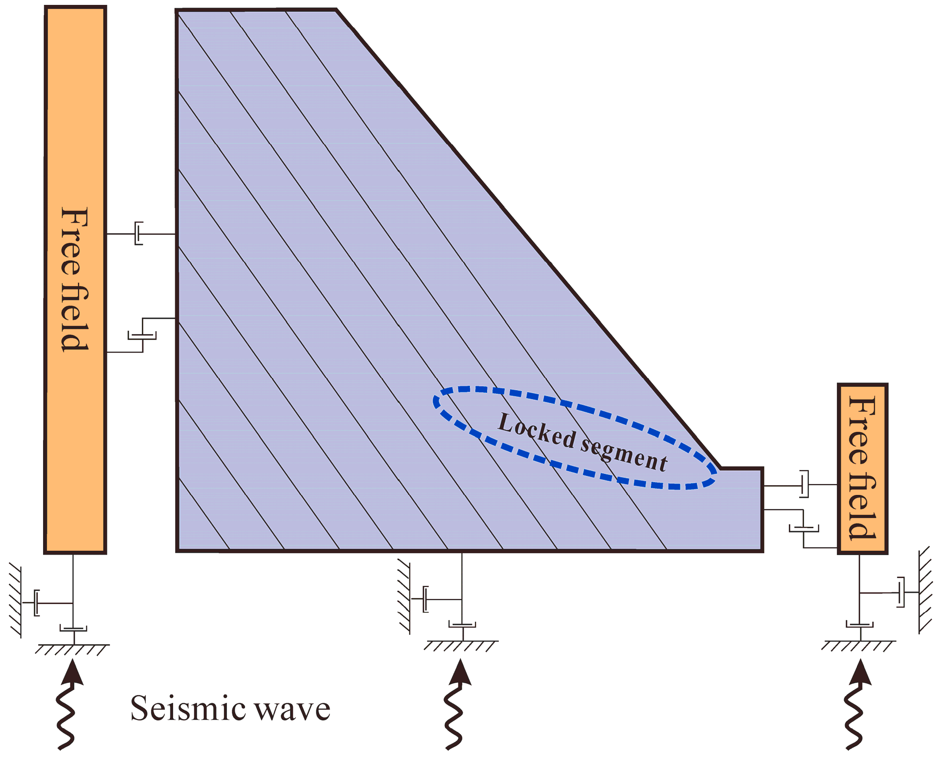
2.2. Boundary Conditions and Loading Conditions

For numerical simulations, boundary conditions are crucial considerations [29]. Figure 3 displays the boundary conditions of the numerical model used in this investigation. The viscous boundary was positioned at the bottom of the model to lessen the impact of seismic wave reflection on the numerical simulation results, while the free-field boundary was positioned around the model to replicate the semi-infinite space.

This study used an integral to convert the seismic wave’s acceleration time history to velocity time history, which was subsequently transformed into stress time history using Formulas (5) and (6). To replicate the seismic action, the seismic wave is entered into the model from the bottom as a stress wave.

$${\sigma }_n=-\left(2\rho C_p\right)v_n,$$

(5)

$${\sigma }_s=-\left(2\rho C_s\right)v_s,$$

(6)

where σ_n is the normal stress (MPa), σ_s is the tangential stress (MPa), ρ is the density of the medium (kg/m³), v_n is the vibration velocity in the lead direction of the input mass (m/s), and vs. is the vibration velocity in the horizontal direction of the input mass (m/s). Additionally, C_p and C_s stand for the seismic P and S wave propagation velocities in rock, respectively. Local damping is chosen in the calculation process to better reflect the real response under seismic action, and the local damping coefficient was set to 0.157 [30,31].

Twenty acceleration monitoring points were positioned at different heights within the slope and along the slope surface, as shown in Figure 4, in order to systematically examine the dynamic response law within the slope. The acceleration response law of the internal measurement sites of the slope from low to high along the elevation was examined in this study using a variety of elevation monitoring points (M5, M10, M14, M17, and M19). The monitoring locations (M6, M5, M4, M3, M2, and M1) at the same elevation were selected in order to investigate the acceleration response law of the measurement stations within the slope from the inside to the outside along the slope direction. The acceleration monitoring point M0 was concurrently positioned above the center of the model’s bottom to verify the accuracy of the incoming seismic wave.

This numerical simulation study uses the Wolong wave as the loading seismic wave, which is consistent with the seismic input wave we employed in our earlier slope shaking table test [20]. The time compression ratio of 1:4 [32] can be computed using the Buckingham similarity relation Formulas (7) and (8). This means that the Wolong wave is compressed four times and used for numerical simulation; Figure 5 displays its time-course curves and spectral curves, and the main frequency of the seismic wave, f₀, which is approximately 13 Hz.

$$C_t=C_l{\left(C_{\rho }/C_E\right)}^{1/2},$$

(7)

$$C_E=C_{\rho }{C}_l,$$

(8)

where C_t is the time similarity ratio, C_l is the length ratio, and C_ρ is the density ratio. According to the load capacity and working frequency of the shaker, the length ratio of the model is taken as 16, and the density ratio of the material is taken as 1.0.

According to the shaker test conditions used in our previous work [20], six different seismic waves with amplitudes of 0.1 g, 0.2 g, 0.3 g, 0.4 g, 0.5 g, and 0.6 g were selected for this numerical simulation investigation. There were six circumstances in all, with all loading directions in the horizontal X-direction.

3. Results and Discussion

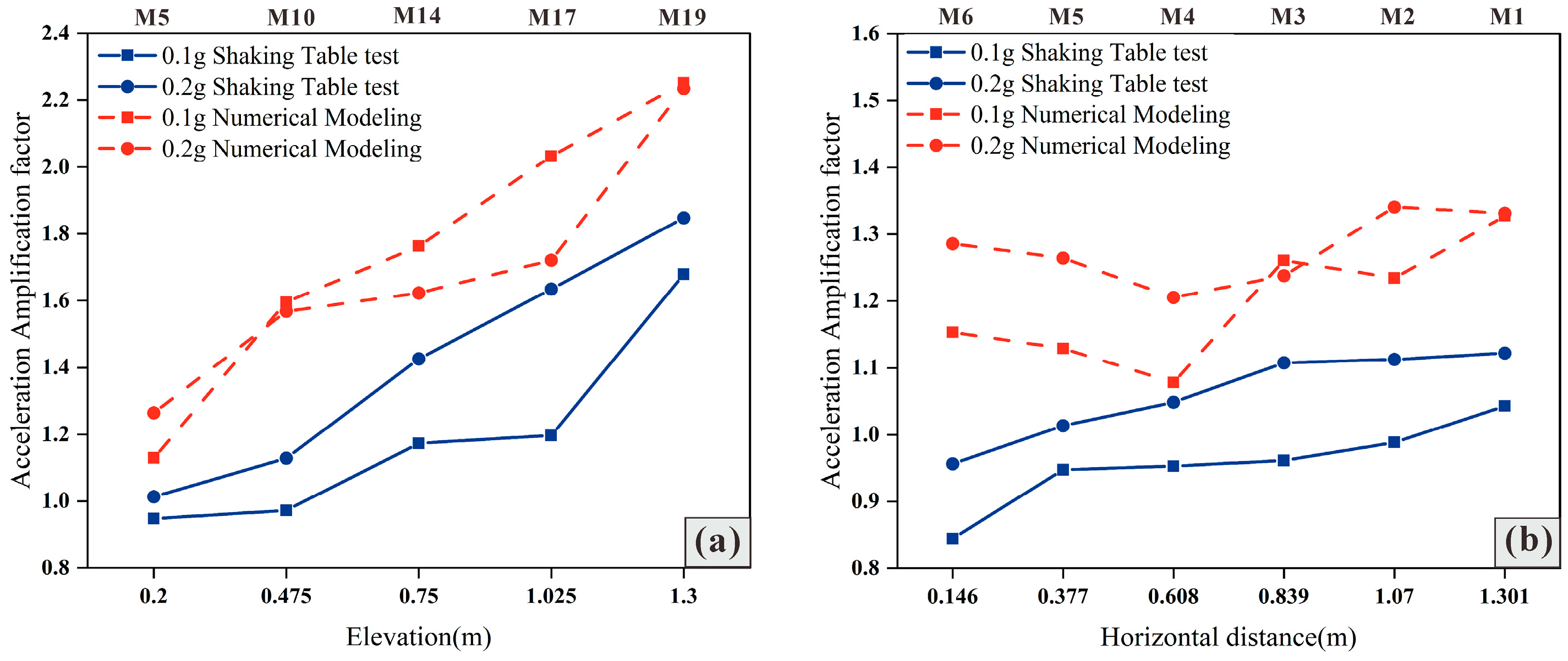
3.1. The Law of Acceleration Response Characteristics

Seismic inertia force is the main cause of slope deformation and failure under earth-quake action. The acceleration amplification factor (AAF), which roughly corresponds to the maximum seismic inertia force experienced by the slope throughout the entire excitation process, is defined as the ratio of the peak acceleration (A_E) of the dynamic response at each measurement point of the slope to the peak acceleration (A_C) of the measured input at the table surface. In this manner, the analysis of the slope’s AAF and its distribution pattern can disclose the deformation properties of the slope under earthquake activity [33]. Furthermore, by contrasting the acceleration amplification coefficients of the shaking table test with the numerical simulation, the accuracy of the latter can be confirmed.

Figure 6 displays the results of a comparative analysis of the AAF obtained from the slope shaker test and numerical simulation under the action of seismic waves of the same amplitude (using 0.1 g and 0.2 g seismic waves as an example). They show that, generally speaking, the variation law of the slope’s AAF from the slope shaker test and the numerical simulation that we previously conducted is the same. Specifically, the AAF at different elevation measurement points within the slope of both showed an overall increasing trend along the elevation from the bottom to the top of the slope (Figure 6a). Simultaneously, the AAF of the same elevation measurement points within the slope of both also showed an overall increasing trend along the slope direction from the interior of the slope to the slope surface (Figure 6b). In other words, the AAF showed an elevation effect and a tendency to surface effect. It should be noted that the boundary conditions on both sides of the X-direction of the model in the shaking table physical model test are insufficient to fully simulate the infinite boundary. As a result, the seismic wave produces reflection waves on both sides of the boundary, interfering with the seismic response inside the slope and producing the difference between the two data. This further demonstrates the superiority of numerical simulations in handling the boundary. As a result, the work that follows is predicated on excellent numerical simulation data.

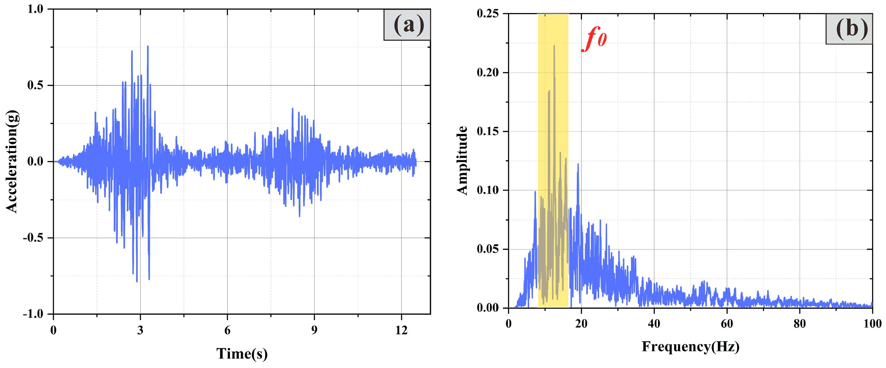
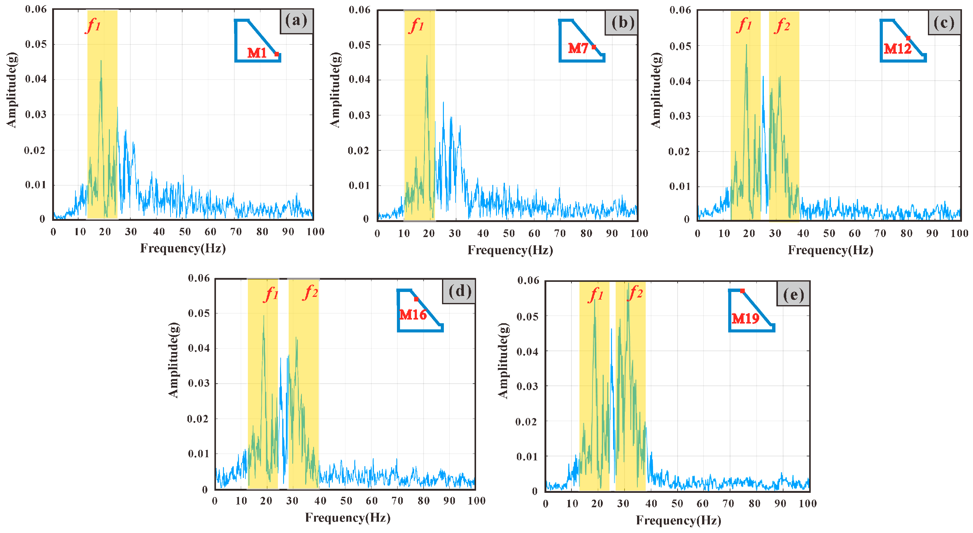
3.2. Fourier Spectrum Analysis of Acceleration

In addition to the previously mentioned seismic inertial force, the frequency change that takes place during the seismic wave transmission process also affects the slope’s dynamic response characteristics, as can be observed by looking at the Fourier spectrum of the slope’s acceleration [34]. Using the Fast Fourier Transform for the signals acquired at different monitoring points, we may accomplish this by transferring the acceleration signals from the time domain to the frequency domain for Fourier spectrum frequency analysis. Meanwhile, Liu et al. [35] showed that when the seismic wave amplitude is more than 0.2 g, the top of the slope tends to produce substantial strains, which lowers the high-frequency response of the seismic wave. In order to fully examine the variable features of the Fourier spectrum under earthquake action, this study focuses on the Fourier spectrum of slope acceleration when the amplitude of the seismic waves is less than 0.2 g.

The spectrum features of the slope surface monitoring locations (M1, M7, M12, M16, and M19) under the action of 0.1 g seismic waves were examined as an example based on the numerical simulation results with superior time continuity. It is evident from the findings in Figure 7 that the slope surface monitoring point’s acceleration rises with elevation. The Fourier spectrum gradually changes from having a single peak (f₁) to having two peaks (f₁ and f₂). The amplitude of the low-frequency peak (f₁), which is near the main frequency of the input seismic wave (f₀) in Figure 5b, does not change much as the elevation rises, while the amplitude of the high-frequency peak (f₂) gradually increases as the elevation rises. This suggests that the Fourier spectrum of the slope acceleration’s amplification impact is selective, which is in line with the findings of earlier research [36].

3.3. Analysis of Hilbert Spectrum

In this subsection, we set up a set of homogeneous slope tests without a weak layer as a control group in order to clearly characterize the internal energy response of the slope under seismic wave action and to deeply reveal the influence of the weak layer on the internal energy changes of the slope under earthquake action. The aforementioned examination of the SBRS model with weak layer served as the basis for this. The two sets of dynamic response data are then compared and evaluated using the HHT to further illustrate the effect of the weak layer on the slope during earthquake activity.

The HHT, a vibration signal processing method that has a high resolution of vibration signals in the time-frequency domain, was introduced by Huang et al. [37] in 1996. It displays the transitory properties of seismic signals. The two primary parts of the HHT are the Hilbert transform and the empirical modal decomposition (EMD). In essence, the EMD decomposes a non-smooth seismic signal into a residual and several intrinsic mod-al functions (IMFs), each of which needs to satisfy the following specifications: (1) The number of extreme points and zero-crossing points must be equal or less than one during the signal duration. (2) The lower envelope based on the local minimum and the higher envelope based on the local maximum both have an average value of zero. Figure 8 illustrates the precise IMF determination procedure. For instance, Figure 9 displays the IMF components and residuals following EMD processing, as well as the acceleration time-range curve of the smooth-layer slope monitoring M1 under the influence of a 0.1 g seismic wave.

The Hilbert transform is applied to each IMF component by Equation (9), and the result is analyzed by Equations (10)–(13) to obtain the Hilbert spectrum, which better reflects the energy distribution and response characteristics of seismic signals in the time–frequency domain.

$$Y(t)={\displaystyle \frac{1}{\pi }}P{\int }_{-\infty }^{\infty }{\displaystyle \frac{x\left(t^{\prime }\right)}{t-t^{\prime }}}\mathrm{d}{t}^{\prime },$$

(9)

$$a(t)={\left[X^2(t)+Y^2(t)\right]}^{1/2},$$

(10)

$$\theta (t)=\arctan \left[{\displaystyle \frac{X(t)}{Y(t)}}\right],$$

(11)

$$\omega (t)={\displaystyle \frac{d\theta (t)}{dt}},$$

(12)

$$H(t,\omega )=R\sum _{j=1}^n{a}_j(t){\mathrm{e}}^{i\int {\omega }_j(t)\mathrm{d}t},$$

(13)

where Y(t) is the result of HHT, P is the value of the Cauchy principal component, x(t) is the original signal, H(t,ω) is the Hilbert spectrum, R is the real part, a_j(t) denotes the magnitude of the jth-order IMF corresponding to the instantaneous frequency ω_j at the moment t and is a constant, a(t) is the instantaneous amplitude, θ(t) is the instantaneous phase, and ω(t) is the instantaneous frequency.

The acceleration signals obtained at various elevation monitoring stations in the SBRS and the homogeneous slope while being impacted by a 0.1 g seismic wave were subjected to EMD and Hilbert transform in this instance. The resultant Hilbert spectrum is displayed in Figure 10 and Figure 11. (1) As can be observed, the distribution range of the Hilbert energy of the monitoring point M5 in the SBRS and the homogeneous slope is primarily concentrated in 2~4 s and 8~10 s on the time axis, respectively, whereas the frequency axis distribution range is primarily concentrated in 10~20 Hz depending on the frequency of the loading seismic wave (Figure 10 and Figure 11). (2) As the elevation of the monitoring points increases, the frequency distribution range of the Hilbert energy at the monitoring points in both models appears to broaden significantly, presumably due to the elevation amplifying the high-frequency portion of the Hilbert energy. It should be noted that the enhancement of Hilbert energy for the homogeneous slope is not obvious and the increase in energy is small (Figure 11), whereas the Hilbert energy for the SBRS (Figure 10) undergoes an enhancement of the energy from 10 Hz to 20 Hz, and the increase in energy increases with the increase in the number of weak layers. This leads us to hypothesize that the reason for this discrepancy is the reflection and refraction of seismic waves via weak strata as they propagate. Furthermore, we discovered that, with a maximum frequency of 30 Hz and a spike of Hilbert energy in the high-frequency portion, monitoring point M19 on the SBRS had the widest Hilbert energy frequency band. This suggests that the top of the slope is likely to sustain damage first during seismic activity because the weak layer of the slope amplifies the Hilbert energy more than the elevation does, and the amplification effect on the high-frequency part of the Hilbert energy is more pronounced.

3.4. Analysis of the Marginal Spectrum

The MSP provides a clearer view of the energy distribution of each seismic signal frequency throughout the whole signal range than the Hilbert spectrum does. The monitoring point’s MSP amplitude at the damage site will grow drastically if the slope structure has a damage crack that seriously compromises its integrity in the event of an earthquake. It is possible to determine the dynamic failure mechanism of the slope structure by evaluating the change in the internal damage fracture of the slope under the impact of an earthquake. The slope failure condition may be examined using the MSP, as seen in Figure 12.

To better understand the damage process of the locked segment under the action of earthquakes, this part calculates the MSP of the lower monitoring point M4 and the higher monitoring point M9 of the locked segment under the excitation of 0.3 g and 0.4 g seismic waves. The results are shown in Figure 13. It is evident that under the two operating situations, the MSPs of the monitoring sites close to the locked segment show two noticeable peaks. The frequency of the first peak, which is primarily spread around 13 Hz, is comparable to the input seismic wave’s main frequency, f₀, as seen in Figure 5b. It can be considered that it is mainly controlled by the loading seismic wave. The second peak is mainly distributed near 18 Hz, and it is speculated that it may be affected by the natural frequency of the slope. Furthermore, the Hilbert energy peak controlled by the main earthquake frequency in the monitoring point’s MSP under the excitation of a 0.4 g seismic wave is significantly higher than that under the excitation of a 0.3 g seismic wave. This suggests that the Hilbert energy of the seismic wave-controlled MSP gradually dominates, indicating that the slope is deformed and damaged. In the meantime, the upper monitoring point M9 of the locked segment has a higher peak value in its MSP Hilbert energy than the lower monitoring point M4 of the locked segment, and the high-frequency band of its MSP has a more noticeable amplification phenomenon (i.e., a sudden increase). This suggests that the internal part of the locked segment has started to produce damage under the action of a 0.4 g seismic wave at this time. Though this is not through actual damage, there is already a precursor.

4. Conclusions

In order to extend the research and methodically uncover the seismic dynamic response characteristics of the steep bedding rock slope (SBRS), this paper has performed a dynamic numerical simulation based on the slope shaking table experiments carried out early in our study. It should be pointed out that we maintained great consistency in the size and physical parameters between the shaking table model and the numerical simulation model throughout the modeling process to guarantee the accuracy of the numerical simulation results. The following conclusions are drawn from a systematic analysis of the dynamic response characteristics of the SBRS under the action of an earthquake from an energy point of view using the Hilbert–Huang transform and marginal spectrum theory:

(1)

The acceleration amplification factor AAF of the slope under seismic action shows an obvious ’elevation effect’ and ’surface effect’. Simultaneously, the slope surface monitoring point’s acceleration Fourier spectrum gradually changes from a single peak to a double peak as its elevation rises. The amplitude of the high-frequency peak is more noticeable with the elevation amplification effect than the low-frequency peak, indicating that the slope acceleration Fourier spectrum’s amplification effect is somewhat selective.

(2)

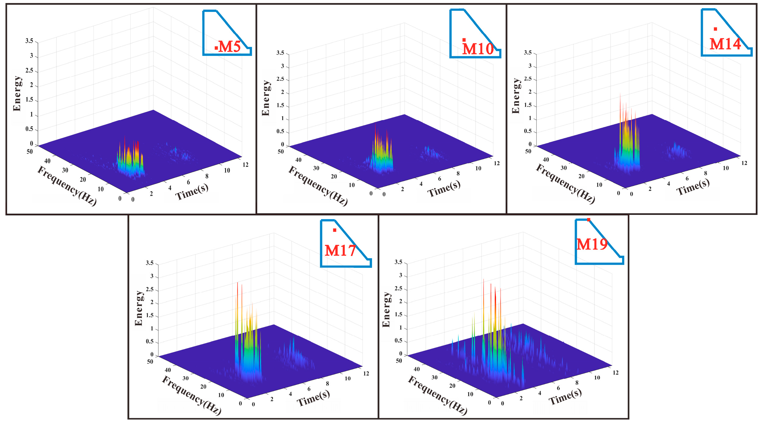
Both the elevation and weak layers amplify the transmission of Hilbert energy, and the comparison of the Hilbert spectrums of an SBRS with weak layers and a homogeneous slope reveals a greater amplification of the high-frequency component of Hilbert energy. Because of this, the weak layer at the top of the slope is often damaged first when an earthquake happens. The final instability of the SBRS results from the progressive extension of the tensile fractures in the slope downhill and the progressive cutting and joining of the locked section at the toe of the slope.

(3)

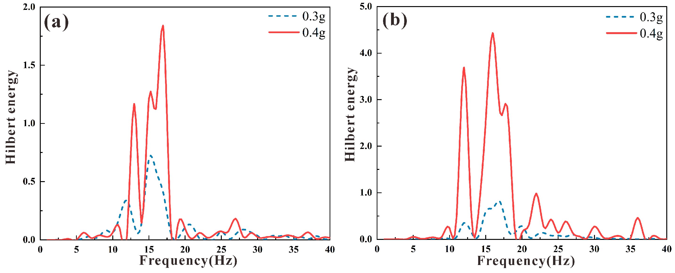
The peak value of the marginal spectrum’s Hilbert energy corresponding to the main earthquake frequency will be considerably boosted as the seismic wave amplitude grows, according to a comparison of the SBRS’s marginal spectrum under different seismic wave amplitudes. This implies that when the Hilbert energy of the marginal spectrum being regulated by seismic waves progressively takes over, the slope is harmed and distorted. Additionally, there is a precursor even though there is no penetration damage because the Hilbert energy in the high-frequency band of the marginal spectrum at the locked segment’s upper monitoring point will suddenly rise before penetration damage occurs in the locked segment close to the base of the slope. This suggests that the top portion of the internal portion of the locked section has begun to sustain damage.

Finally, we have not been able to provide a universal index that would enable us to identify the unstable area of this type of slope, even though this article has extensively investigated the dynamic response characteristics of the SBRS from an energy perspective using the Hilbert–Huang transform and marginal spectrum theory. In order to predict when this kind of slope would become unstable, we will try to evaluate its condition using a specific energy index in our future studies.

References

1. Wang, X.; Chen, L.; Chen, Q.-F. Evaluation of 3D Crustal Seismic Velocity Models in Southwest China: Model Performance, Limitation, and Prospects. Sci. China Earth Sci. 2024, 67, 604–619. [Google Scholar] [CrossRef]
2. Yao, H.; Liu, Y.; Zhang, Z. CSES Community Velocity Models in Southwest China. In China Seismic Experimental Site: Theoretical Framework and Ongoing Practice; Li, Y.-G., Zhang, Y., Wu, Z., Eds.; Springer Nature: Singapore, 2022; pp. 53–90. ISBN 9789811686078. [Google Scholar]
3. Wang, Y.; Ling, Y.; Chan, T.O.; Awange, J. High-Resolution Earthquake-Induced Landslide Hazard Assessment in Southwest China through Frequency Ratio Analysis and LightGBM. Int. J. Appl. Earth Obs. Geoinf. 2024, 131, 103947. [Google Scholar] [CrossRef]
4. Dai, L.; Fan, X.; Wang, X.; Fang, C.; Zou, C.; Tang, X.; Wei, Z.; Xia, M.; Wang, D.; Xu, Q. Coseismic Landslides Triggered by the 2022 Luding Ms6.8 Earthquake, China. Landslides 2023, 20, 1277–1292. [Google Scholar] [CrossRef]
5. Qin, Y.; Zhang, D.; Zheng, W.; Yang, J.; Chen, G.; Duan, L.; Liang, S.; Peng, H. Interaction of Earthquake-Triggered Landslides and Local Relief: Evidence from the 2008 Wenchuan Earthquake. Landslides 2023, 20, 757–770. [Google Scholar] [CrossRef]
6. Li, L. Seismic Stability of Steep Consequent Rockslides with Different Lithology Assemblies: A Comparative Study. Bull. Eng. Geol. Environ. 2024, 83, 353. [Google Scholar] [CrossRef]
7. Xia, C.; Shi, Z.; Liu, M.; Li, B.; Yu, S.; Xue, J. Dynamic Analysis of Field-Scale Rockslides Based on Three-Dimensional Discontinuous Smoothed Particle Hydrodynamics: A Case Study of Tangjiashan Rockslide. Eng. Geol. 2024, 336, 107558. [Google Scholar] [CrossRef]
8. Yang, J.; Shi, Z.; Peng, M.; Zheng, H.; Soares-Frazão, S.; Zhou, J.; Shen, D.; Zhang, L. Quantitative Risk Assessment of Two Successive Landslide Dams in 2018 in the Jinsha River, China. Eng. Geol. 2022, 304, 106676. [Google Scholar] [CrossRef]
9. Zhang, X.; Chen, X.; Liu, W.; Hu, M.; Dong, J. The Comprehensive Risk Assessment of the Tangjiashan Landslide Dam Incident, China. Environ. Sci. Pollut. Res. 2023, 30, 73913–73927. [Google Scholar] [CrossRef]
10. Chen, X.Q.; Cui, P.; Li, Y.; Zhao, W.Y. Emergency Response to the Tangjiashan Landslide-Dammed Lake Resulting from the 2008 Wenchuan Earthquake, China. Landslides 2011, 8, 91–98. [Google Scholar] [CrossRef]
11. Pei, X.; Cui, S.; Liang, Y.; Wang, H. The Multiple Earthquakes Induced Progressive Failure of the Xinmo Landslide, China: Based on Shaking Table Tests. Environ. Earth Sci. 2023, 82, 465. [Google Scholar] [CrossRef]
12. Chen, J.; Che, A.; Wang, L.; Zhou, H. Investigating the Failure Mechanism of Loess-Mudstone Landslides with a High Water Content Interface Subjected to Earthquakes through the Shaking Table Test. Soil Dyn. Earthq. Eng. 2024, 177, 108406. [Google Scholar] [CrossRef]
13. Feng, Z.-Y.; Lu, Y.-R.; Shen, Z.-R. A Numerical Simulation of Seismic Signals of Coseismic Landslides. Eng. Geol. 2021, 289, 106191. [Google Scholar] [CrossRef]
14. Li, L.; Xue, L.; Jiang, T.; Huang, K.; Li, Z. A Study on the Dynamic Response and Deformation of Slopes Supported by Anti-Slide Piles Subjected to Seismic Waves with Different Spectral Characteristics. Sustainability 2024, 16, 9623. [Google Scholar] [CrossRef]
15. Wang, J.; Wu, Z.; Shi, X.; Yang, L.; Liu, R.; Lu, N. Exploring Mechanism of Hidden, Steep Obliquely Inclined Bedding Landslides Using a 3DEC Model: A Case Study of the Shanyang Landslide in Shaanxi Province, China. China Geol. 2024, 7, 303–314. [Google Scholar] [CrossRef]
16. Xin, C.; Yang, F.; Feng, W.; Wang, Z.; Li, W. Seismic Responses and Shattering Cumulative Effects of Bedding Parallel Stepped Rock Slope: Model Test and Numerical Simulation. J. Rock Mech. Geotech. Eng. 2024, 6, 1614. [Google Scholar] [CrossRef]
17. Tan, X.; Ren, Y.; Li, T.; Zhou, S.; Zhang, J.; Zhou, S. In-Situ Direct Shear Test and Numerical Simulation of Slate Structural Planes with Thick Muddy Interlayer along Bedding Slope. Int. J. Rock Mech. Min. Sci. 2021, 143, 104791. [Google Scholar] [CrossRef]
18. Wang, C.; Guo, M.; Chen, X.; Gu, K.; Gong, Y.; Qi, Y.; Yuan, D.; Zhu, C.; Chen, B. Damage Evolution of the Bedding Rock Landslide and Debris Landslide under Earthquakes in the Three-Rivers Basin. Eng. Geol. 2024, 339, 107631. [Google Scholar] [CrossRef]
19. Zang, M.; Yang, G.; Dong, J.; Qi, S.; He, J.; Liang, N. Experimental Study on Seismic Response and Progressive Failure Characteristics of Bedding Rock Slopes. J. Rock Mech. Geotech. Eng. 2022, 14, 1394–1405. [Google Scholar] [CrossRef]
20. Dong, J.; Wang, C.; Huang, Z.; Yang, J.; Xue, L. Shaking Table Model Test to Determine Dynamic Response Characteristics and Failure Modes of Steep Bedding Rock Slope. Rock Mech. Rock. Eng. 2022, 55, 3645–3658. [Google Scholar] [CrossRef]
21. Garcia, S.R.; Romo, M.P.; Alcántara, L. Analysis of Non-Linear and Non-Stationary Seismic Recordings of Mexico City. Soil Dyn. Earthq. Eng. 2019, 127, 105859. [Google Scholar] [CrossRef]
22. Fan, G.; Zhang, J.; Wu, J.; Yan, K. Dynamic Response and Dynamic Failure Mode of a Weak Intercalated Rock Slope Using a Shaking Table. Rock Mech. Rock Eng. 2016, 49, 3243–3256. [Google Scholar] [CrossRef]
23. Fan, G.; Zhang, L.-M.; Zhang, J.-J.; Ouyang, F. Energy-Based Analysis of Mechanisms of Earthquake-Induced Landslide Using Hilbert–Huang Transform and Marginal Spectrum. Rock Mech. Rock Eng. 2017, 50, 2425–2441. [Google Scholar] [CrossRef]
24. Song, D.; Chen, Z.; Chao, H.; Ke, Y.; Nie, W. Numerical Study on Seismic Response of a Rock Slope with Discontinuities Based on the Time-Frequency Joint Analysis Method. Soil Dyn. Earthq. Eng. 2020, 133, 106112. [Google Scholar] [CrossRef]
25. Song, D.; Liu, X.; Huang, J.; Zhang, J. Energy-Based Analysis of Seismic Failure Mechanism of a Rock Slope with Discontinuities Using Hilbert-Huang Transform and Marginal Spectrum in the Time-Frequency Domain. Landslides 2021, 18, 105–123. [Google Scholar] [CrossRef]
26. Chen, J.; Wang, L.; Wang, P.; Che, A. Failure Mechanism Investigation on Loess–Mudstone Landslides Based on the Hilbert–Huang Transform Method Using a Large-Scale Shaking Table Test. Eng. Geol. 2022, 302, 106630. [Google Scholar] [CrossRef]
27. Lei, H.; Wu, H.; Qian, J. Seismic Failure Mechanism and Interaction of the Cross Tunnel-Slope System Using Hilbert-Huang Transform. Tunn. Undergr. Space Technol. 2023, 131, 104820. [Google Scholar] [CrossRef]
28. Kuhlemeyer, R.L.; Lysmer, J. Finite Element Method Accuracy for Wave Propagation Problems. J. Soil Mech. Found. Div. 1973, 99, 421–427. [Google Scholar] [CrossRef]
29. Qi, S.; He, J.; Zhan, Z. A Single Surface Slope Effects on Seismic Response Based on Shaking Table Test and Numerical Simulation. Eng. Geol. 2022, 306, 106762. [Google Scholar] [CrossRef]
30. Xue, L.; Li, L.; Xu, C.; Cui, Y.; Ding, H.; Huang, K.; Li, Z. A Multi-Objective Optimization Evaluation Model for Seismic Performance of Slopes Reinforced by Pile-Anchor System. Sci. Rep. 2024, 14, 5044. [Google Scholar] [CrossRef] [PubMed]
31. Antwi Buah, P.; Zhang, Y.; He, J.; Yu, P.; Xiang, C.; Fu, H.; He, Y.; Liu, J. Evaluating the Dynamic Response and Failure Process of a Rock Slope under Pulse-like Ground Motions. Geomat. Nat. Hazards Risk 2023, 14, 2167613. [Google Scholar] [CrossRef]
32. Buckingham, E. On Physically Similar Systems; Illustrations of the Use of Dimensional Equations. Phys. Rev. 1914, 4, 345–376. [Google Scholar] [CrossRef]
33. Tai, D.; Qi, S.; Zheng, B.; Luo, G.; He, J.; Guo, S.; Zou, Y.; Wang, Z. Effect of Excitation Frequency and Joint Density on the Dynamic Amplification Effect of Slope Surface on Jointed Rock Slopes. Eng. Geol. 2024, 330, 107385. [Google Scholar] [CrossRef]
34. Nussbaumer, H.J. The Fast Fourier Transform. In Fast Fourier Transform and Convolution Algorithms; Nussbaumer, H.J., Ed.; Springer: Berlin/Heidelberg, Germany, 1982; pp. 80–111. ISBN 978-3-642-81897-4. [Google Scholar]
35. Liu, H.; Xu, Q.; Li, Y.; Fan, X. Response of High-Strength Rock Slope to Seismic Waves in a Shaking Table Test. Bull. Seismol. Soc. Am. 2013, 103, 3012–3025. [Google Scholar] [CrossRef]
36. Song, D.; Che, A.; Chen, Z.; Ge, X. Seismic Stability of a Rock Slope with Discontinuities under Rapid Water Drawdown and Earthquakes in Large-Scale Shaking Table Tests. Eng. Geol. 2018, 245, 153–168. [Google Scholar] [CrossRef]
37. Huang, N.E.; Long, S.R.; Shen, Z. The Mechanism for Frequency Downshift in Nonlinear Wave Evolution. In Advances in Applied Mechanics; Hutchinson, J.W., Wu, T.Y., Eds.; Elsevier: Amsterdam, The Netherlands, 1996; Volume 32, pp. 59–117, 117A, 117B, 117C. [Google Scholar]
Figure 1. The steep bedding rock slope model. (unit: mm).
Applsci 15 03078 g001
Figure 2. Numerical model of the slope. (unit: mm).
Applsci 15 03078 g002
Figure 3. Boundary conditions of numerical simulation.
Applsci 15 03078 g003
Figure 4. Monitoring point layout. (unit: mm).
Applsci 15 03078 g004
Figure 5. Time history curve and Fourier spectrum of 4 seismic wave compressed 4 times: (a) time history curve and (b) Fourier spectrum.
Applsci 15 03078 g005
Figure 6. AAF response law: (a) AAF response law along elevations at different elevation monitoring points in the slope; (b) AAF response law along slope directions at the same elevation monitoring points in the slope.
Applsci 15 03078 g006
Figure 7. Fourier spectrum of different monitoring points on slope surface under action of 0.1 g seismic wave: (a) Fourier spectrum of monitoring point M1. (b) Fourier spectrum of monitoring point M7. (c) Fourier spectrum of monitoring point M12. (d) Fourier spectrum of monitoring point M16. (e) Fourier spectrum of monitoring point M19.
Applsci 15 03078 g007
Figure 8. Flowchart of EMD method.
Applsci 15 03078 g008
Figure 9. IMF component time-course curves and residuals for monitoring point M1.
Applsci 15 03078 g009
Figure 10. Time history curves and 3D Hilbert spectra of steep bedding rock slope at different monitoring points under action of 0.1 g seismic wave.
Applsci 15 03078 g010
Figure 11. Time history curves and 3D Hilbert spectra of homogeneous slope at different monitoring points under action of 0.1 g seismic wave.
Applsci 15 03078 g011
Figure 12. Steps of slope damage state study using marginal spectra.
Applsci 15 03078 g012
Figure 13. Marginal spectra of monitoring points under action of seismic waves of different amplitudes: (a) marginal spectrum of monitoring point M4 and (b) marginal spectrum of monitoring point M9.
Applsci 15 03078 g013